Abstract
Self-driving cars, i.e., fully automated cars, will spread in the upcoming two decades, according to the representatives of automotive industries; owing to technological breakthroughs in the fourth industrial revolution, as the introduction of deep learning has completely changed the concept of automation. There is considerable research being conducted regarding object detection systems, for instance, lane, pedestrian, or signal detection. This paper specifically focuses on pedestrian detection while the car is moving on the road, where speed and environmental conditions affect visibility. To explore the environmental conditions, a pedestrian custom dataset based on Common Object in Context (COCO) is used. The images are manipulated with the inverse gamma correction method, in which pixel values are changed to make a sequence of bright and dark images. The gamma correction method is directly related to luminance intensity. This paper presents a flexible, simple detection system called Mask R-CNN, which works on top of the Faster R-CNN (Region Based Convolutional Neural Network) model. Mask R-CNN uses one extra feature instance segmentation in addition to two available features in the Faster R-CNN, called object recognition. The performance of the Mask R-CNN models is checked by using different Convolutional Neural Network (CNN) models as a backbone. This approach might help future work, especially when dealing with different lighting conditions.
1. Introduction
Previous studies presented that energy minimization is a critical area of autonomous transport system development, where advanced longitudinal and lateral vehicle control methods will play a key role in achieving expected results [1,2,3,4,5,6,7]. Conversely, numerous research papers propose to improve the efficiency of the vehicle control process through the development of sensor systems and image detection methods [8,9,10,11]. Based on this, we understand that image detection approaches can directly affect the efficiency of highly automated transport systems. In light of this, our paper discusses the comparison of different models influencing the efficiency of image detection processes.
The recent trends in self-driving cars have encouraged researchers to use several object detection algorithms that include various areas in self-driving cars, such as pedestrian detection (see Figure 1) [12,13,14,15], lane detection, traffic signal detection [16], and many more. Due to the recent development in CNN and its outstanding performance in these state-of-the-art visual recognition solutions, these processes have become increasingly intensive. CNN is basically used for image classifying tasks, but it cannot detect objects. For this purpose, many object detection algorithms are available, for instance, SSD (Single Shot Multibox Detector) [14,15,16,17] YOLO (You Only Look Once) [18,19,20,21], R-CNN [10], and Fast R-CNN [22,23]. All object detection models localize objects by using bounding boxes and classifying them by labels.
This paper focuses on pedestrian detection, especially in different visibility conditions. The developed dataset is manipulated with the inverse gamma correction method to create images representing the different lighting conditions. After this development phase, the Mask R-CNN model [24,25,26,27,28] is trained with this dataset by transfer learning and fine-tuning techniques [29].
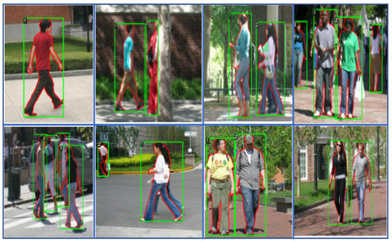
Figure 1.
Pedestrian detection using Mask R-CNN with Resnet50 as a backbone, which runs at epoch10. Developed from [30].
Figure 1.
Pedestrian detection using Mask R-CNN with Resnet50 as a backbone, which runs at epoch10. Developed from [30].

There are relevant difficulties related to pedestrian detection [31] from an automated driving point of view, especially when we consider the experiences of highly automated vehicles’ accidents. For instance, one of the most famous accidents related to highly automated driving is the well-known Arizona-Uber accident [32,33], where the failure of the detection was seriously affected by lighting conditions. Visibility is the most important factor, such as darkness, brightness, and glaring.
2. Literature Review
This paper gives a review of R-CNN models and their variations. The localization process starts with the coarse scan of the whole image and concentrates on the region of interest, where the sliding window method is used to predict the bounding boxes.
Ross Girshick proposed the R-CNN model in 2014 [23]. He developed a selective search method to create 2000 regions for each image called region proposal. It makes the quality of the bounding box better and helps the CNN model extract high-level features. Thus, R-CNN models take the image as the input, and then a 2k region is proposed by a selective search method. After this, it is cropped to a fixed size, called a warped region. Finally, with the CNN model’s help, objects are localized and classified within the region of interest. The CNN model uses the Linear Support Vector Machine (SVM) method [33] to classify the classes of objects as well as non-max suppression methods [16] to suppress the bounding boxes that have a value of less than the critical value.
In other words, R-CNN consists of four processes. First, regions are proposed in the image with the selective method, and then it is warped in a fixed size. After that, the warped region is fed in the CNN model with a fixed size of 227 × 227 pixels to classify and predict bounding boxes. It extracts 4096 feature vectors from each region proposal. The image contains objects with different sizes and aspect ratios; thus, the region proposal feature comes in different sizes. Before feeding into the CNN model, it is cropped and warped.
The R-CNN method has reasonable limitations in terms of training time, since it takes a huge amount of time to classify the 2 k region proposals in each image. At the same time, it must be mentioned that the selective search algorithm is not a self-learning approach. Thus, to solve this problem, Girshick proposed the fast R-CNN model.
The Fast R-CNN model is nine times faster than the R-CNN model [22,23], in which the VGG16 (Visual Geometry Groups 16) [23] approach is used as the backbone. The architecture is the same as the previous model. However, the input image is fed first into the CNN, and then region proposals are applied to the proposed region. After that, region features are warped with the help of the RoI pooling layer. Then, it is reshaped in fixed size to feed into fully connected layers. Similar to the R-CNN, the 2k region is proposed to CNN every time, but in fast R-CNN, it is fed at once.
A high computational complexity can characterize R-CNN and Fast R-CNN models because both use selective search methods to propose the region. Thus, Shaoqing Ren and his team [22,34] created the idea of a Region Proposal Network (RPN) that replaces the selective search region proposal method. In faster R-CNN, the image is fed into the CNN model first to provide a feature map. A separate Region Proposal Network is then used to predict region proposal, which is further reshaped by using RoI pooling. At last, it is classified and labeled in the Region of Interest.
3. Mask R-CNN
The Mask R-CNN concept [24,25,27,28] is the extended version of the fast R-CNN model. It is used to predict a mask that works parallel to the existing branch of classification and bounding box detection in each region of interest. Because of its simplicity, flexibility, and robustness, Kaiming He and his team won the COCO challenge in 2016. This detection system uses one extra feature called RoI Align, which removes the harsh quantization in RoI Pool.
Mask R-CNN has a similar structure to Fast R-CNN. One additional feature is added, called segmentation masks, that work parallel to each region of interest (RoI) to predict the mask, pixel by pixel. Thus, Mask R-CNN gives one extra output, namely masking, including two existing output: class labelling and bounding box. Mask is quite different from the output mentioned above because it extracts the feature pixel by pixel alignment. Thus, it places a colourful layer (mask) on the object, which is the same in size as the object. At the same time, the bound box has a different aspect ratio that predicts the object through the rectangular box, which is always bigger in size than the instances available in the images.
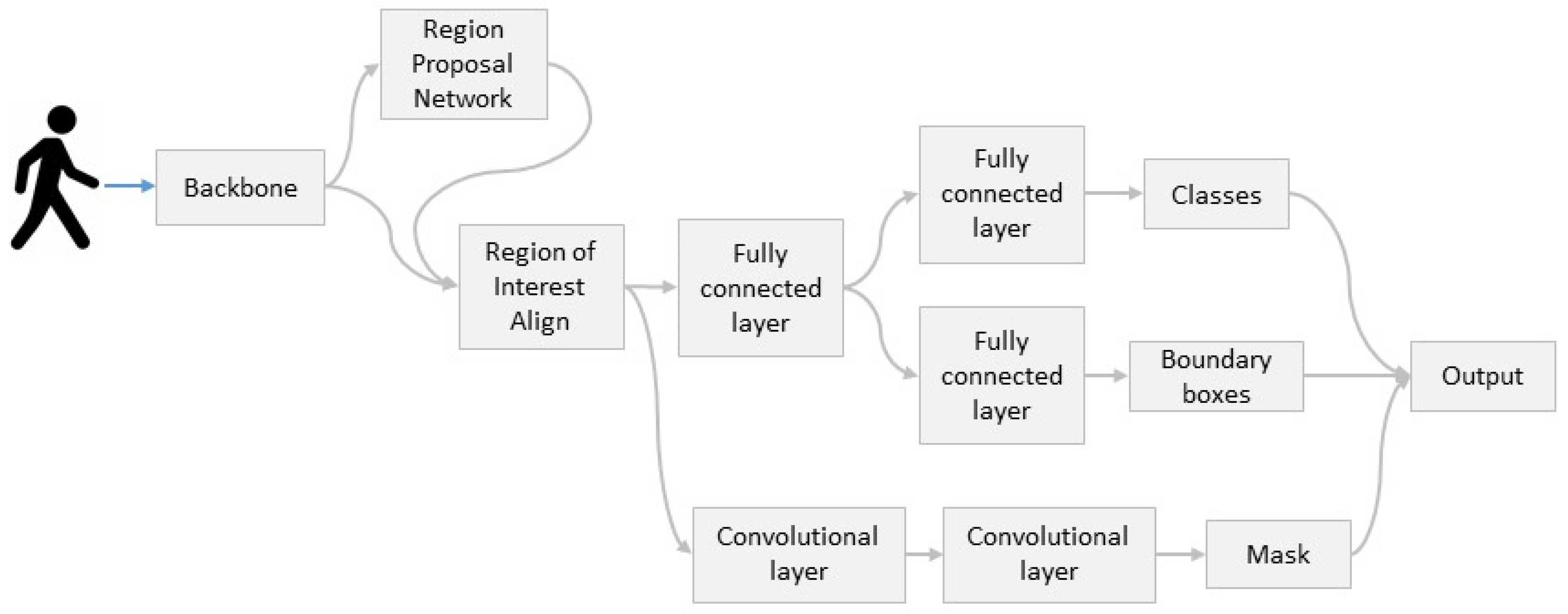
The Mask R-CNN model is a two-stage detection model. The first stage is designed to provide a proposal for the availability of the object with the help of the Region proposal Network (RPN) [22,35], which is similar to what is used in Fast R-CNN. In the second stage, masking is applied in parallel with the class and bounding box, and it gives a binary mask as an output for each RoI, as shown in Figure 2.
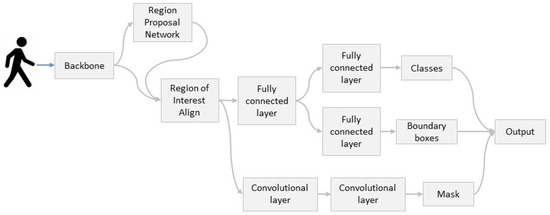
Figure 2.
Architecture diagram of Mask R-CNN detection model.
Figure 2 shows that the input image is fed into the convolution neural network to extract the object features. Mask R-CNN uses a new feature called Region of Interest (Roi) Align [32]. This new feature removes the harsh quantization of the RoI Pool. Then, further convolution layers are used to predict instance segmentation, which works in parallel with the classification and localization of objects in each region of interest.
4. Methodology
This section presents the applied methodological approaches related to improving the efficiency of neural network-based detection models. We first describe the concepts of transfer learning and fine-tuning, as these methods are fundamental for improving the efficiency of an existing detection network. In light of the above, by comparing the backbone network types described below, we have the opportunity to determine the network structure that best supports our goals.
4.1. Transfer Learning and Fine Tuning
In the case of transfer learning [36,37,38,39], the pre-trained models are applied in the solution of various problems by manipulating relevant layers of the network according to the new application’s requirements. In this methodology, some layers are placed in freeze conditions. Fine-tuning is different from transfer learning, where all the layers are used and trained again according to the new application requirements.
This paper uses both techniques to detect the object using Mask R-CNN, where transfer learning techniques replace the backbone. Two classes replace the output of the Mask R-CNN, because the dataset contains two classes, background and masking (foreground), and it is trained again with the help of fine tuning [33,36,40].
4.2. Backbones
As we explained above, the backbone [41] of the Mask R-CNN is a convolution neural network. We tested six different backbone models in the feature extracting and the bounding box identification process. Each Mask R-CNN model with different backbones is trained in different lighting conditions. Since it was not possible to generate the applied dataset during the research, the training and the test procedure was based on a previously developed image dataset (such as images with day or night conditions). In accordance with this, we used a limited number of images from an external database, and we applied the inverse gamma correction method to transform the images into the required lighting conditions. Inverse Gamma Correction Method (IGCM) changes the pixel values to make the picture bright or dark. Each convolutional neural network takes an image with 559 × 536 pixels as an input and provides a 256-channel output connected to the region proposal network. Accordingly, RPN takes 256 channels as input. Thus, all backbone models are modified according to the input channel of the RPN. In this case, transfer learning and fine-tuning methods are used. Accordingly, we briefly describe the different feature extracting models below.
4.2.1. Alex Net
Alex Net was developed by Alex Krizhevsky and his team in 2012 [42,43,44,45,46]. That year, they won the ImageNet Challenge in visual object recognition. In their approach, recognition refers to the prediction of the bounding boxes and the labelling process of the identified objects in the image. It contains five convolution layers and three fully connected layers to extract the features. In the present paper, we made modifications; for instance, we removed all the fully connected layers. After that, we changed the fifth convolution layer’s output, whose channels are equal to the RPN convolution layer’s input.
4.2.2. Mobile Net V2
Mobile Net V2 is the extended version of the Mobile Net V1 method [14], which uses an extra layer called a 1 × 1 expansion layer in each block as compared to Mobile Net V1. Mobile Net V2 [14,17,33,47] replaces the large convolution layer with a depth-wise separable convolution block, and each block contains a 3 × 3 depth wise kernel to filter the output. Further, it is followed by a 1 × 1 point wise convolution layer. Thus, it combines the filters and gives new features. Overall, Mobile Net V1 uses 13 depth-wise separable convolution blocks, preceded by a 3 × 3 regular convolution layer.
At the same time, Mobile Net V2 uses a 1 × 1 expansion layer in each block in addition to the depth wise and pointwise convolution layer. The pointwise convolution layer is also known as the projection layer because it connects a high number of channels with a low number of channels. Furthermore, the 1 × 1 expansion layer expands the channel number before going into the depth-wise convolution layer. This model uses new features called residual connection that help in following the gradient through the neural network. Each block contains batch normalization and ReLU6 activation function, but the projection layer does not use the activation function as an output. This model contains 17 residual blocks, and each block contains depth-wise, pointwise, and 1 × 1 expansion layers. The depth-wise convolution layer is followed by Batch Normalization and Relu6 activation function.
4.2.3. ResNet50
The ResNet model [38,45,46,47] is based on learning the residual instead of learning the low- or high-level features, i.e., residual network. It is used to go deeper and solve complex problems. Thus, ResNet 50 uses 50 residual blocks [48,49,50].
4.2.4. VGG11
Karen Simonyan and Andrew Zisserman introduced this model in 2014 [51]. Their team secured first and second place in the localization and classification problems. This model has eight convolution layers and three fully connected layers. However, in our case, we used only the first four layers of this network.
4.2.5. VGG13
One year later, Simonyan and Zisserman, in 2015 [51], investigated the effect of increasing the layers’ depth. This model contains eleven convolution layers and three fully connected layers, where a 3 × 3 kernel is applied on each convolution layer with a stride 1 × 1 followed by a max pool layer after every two convolution layers.
4.2.6. VGG16
This network [52,53,54] consists of thirteen convolution layers and three fully connected layers, where 3 × 3 filters are used in each convolution layer with a stride size of 1 × 1 and the same padding. Thus, the first two convolution layers contain 64 3 × 3 kernels. The input image fed into the first layer has a size of 224 × 224 × 64. It passes through the second layer, and then max pooling is applied to make the channel double. Thus, the third and fourth layers contain 128 3 × 3 kernels.
Again, the max pool layer is attached to make the channel double. This process is repeated through thirteen layers. The following layers are fully connected that contain 4096 units. These are followed by SoftMax to different 1000 classes. However, we must mention that our investigation considers only convolution layers. It removes the fully connected layers.
As mentioned above, for the three different VGG models, the model’s accuracy increases with the depth of the model. The error rate of these three VGG models is introduced in Table 1 below.

Table 1.
Error rate of variants of VGG models taken from the paper of VGG 11, 13, and 16 models.
5. Dataset
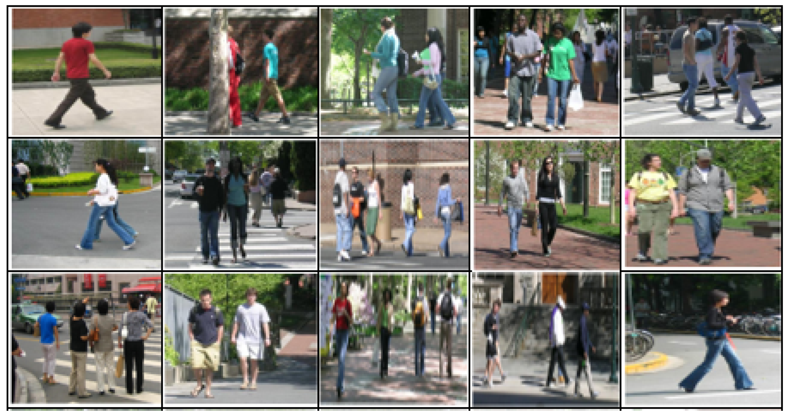
This paper uses the Penn-Fudan Database for pedestrian detection as well as segmentation (see Figure 3), which is available on the website (https://www.kaggle.com/jiweiliu/pennfudanpe, accessed on 1 February 2021). It contains 170 images with 345 pedestrian objects, and it is compatible with both COCO [55,56,57] and Pascal VOC format [54]. We used the dataset during our research in COCO format.

Figure 3.
Pedestrian dataset. Developed from [30].
The database consists of three subfiles, namely Annotation, PedMasks, and PNGImages, where annotation files are in text format, and both PNGImages & PedMasks are in png format. Before applying a Mask R-CNN model, the dataset is pre-processed. Each image is normalized and resized to equal sizes, as shown in Table 2 and Table 3 below, where the normalization process transforms the pixel value of the images into the range of 0 to 1.
Table 2.
The data that is shown in table (a) and (b) are used to modify the images before importing into the models. (a) Normalization of the dataset before importing into the model; (b) resizing of all the images in the dataset. Developed from [58].
Table 3.
Here, Mask R-CNN with different backbones is trained with pedestrian dataset at epoch 10. In a Mask R-CNN, one extra loss called mask loss is added in addition to the losses in faster R-CNN model, where = loss of classifier, = loss of box regression, loss of mask, = objectiveness loss, = loss of RPN box, and = overall loss (the minimum values of the columns are denoted by *).
The table below (Table 3) introduces the results, where the overall loss [24] indicates the sum of all losses.
Equation (1): Total loss () is equal to the sum of all losses.
6. Inverse Gamma Correction
The modification of the luminance characteristics can cause reduced visibility of an object and decrease the detection capability of the system [59]. However, the effect of the lighting conditions depends on many other factors, such as the distance of the given object. Beyond this, the lighting contrast between the object and background can also significantly influence detection efficiency. Accordingly, the system can capture sometimes darker or sometimes brighter images depending on the related factors.
Many different algorithms can be used to adjust the contrast and increase or decrease the brightness of the image. For instance, Histogram Equalization (HE) [60] or Bi-Histogram Equalization (BBHE) [61] can be applied to modify the lighting-related characteristics of the investigated images.
This paper uses the inverse gamma correction method to modify the brightness and darkness of the images. Thus, inverse gamma correction transforms the lighting characteristics of the input signal by applying a nonlinear power function. The power coefficient (gamma) represents the nonlinear nature of the human perception process related to the lighting conditions. Accordingly, the inverse gamma correction transformation is given by Equation (1) below.
Equation (2): Equation of Gamma Inverse Method, where is the output intensity and is the input intensity.
The value of is between 0 and 1, following the introduced model, and is the transformed intensity. This formula is applied when gamma’s value is known, and it is commonly determined experimentally.
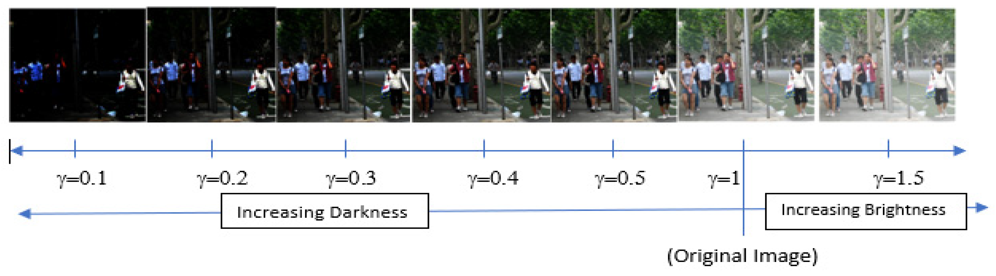
In accordance with the blind inverse gamma correction techniques [61,62,63], gamma is varied between 0.1 and 1.5 with a step size of 0.1, as shown in Figure 4 below. Following this, the gamma value of this image is one. The brightness of the image increases as the gamma value becomes larger, and the image becomes darker as the gamma value decreases.

Figure 4.
The brightness of the image increases when increasing the gamma value (), and it decreases when decreasing the gamma value. Here Gamma Inverse Method is applied to change the luminance intensity of the image. Developed from [30].
7. Instance Segmentation
The instance segmentation [35,58] process involves two main steps. First, it detects and indicates the object by bounding boxes within defined categories, and in the second step, segmentation prediction is performed pixel-wise. Instance segmentation (see Figure 5) is different from semantic segmentation since, beyond the object detection phase, instance segmentation labels the objects, according to the investigated categories’ sub-classes. In contrast, semantic segmentation performs the detection and then classifies the objects. We used the method of instance segmentation with Mask R-CNN in our research. This paper uses instance segmentation with Mask R-CNN.
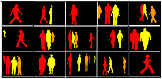
Figure 5.
Instance segmentation of the images where GIMP tool is used to segment the images.
8. Results
The gamma value of the used dataset is assumed to be 1 and is in accordance with the observed good, day-light conditions of the included images. The dataset was augmented by the Torch vision 0.3 package’s inbuilt processing methods of the PyTorch Framework. First, the dataset was converted into a tensor since PyTorch accepts this structure during the pre-processing phase. In the next step, the dataset was loaded in the framework with a batch size number 2. After this, the Mask R-CNN model is applied, which is an inbuilt module of the Torch Vision packages. The Mask R-CNN model works on top of the faster R-CNN detection model. It uses one extra feature called mask prediction that is applied parallel to the object recognition system in each region of interest.
Here, the mask R-CNN model’s backbone is changed with different CNN pre-trained models through the transfer learning technique. In the figure below (see Figure 6), it can be observed that ResNet50 has the lowest loss as compared to other models, whereas VGG16 has the highest loss. In this Mask R-CNN model, anchor boxes are used with a size (32, 64, 128, 256, 512) where region proposal network generates three different aspect ratios, namely 0.5, 1.0, and 2.0. Apart from this, the number of epochs was 10 during the training, and it is optimized with the Stochastic Gradient Descent Method. Parameter values related to the learning method, the momentum, and the weight decay were 0.005, 0.9, and 0.0005, respectively.
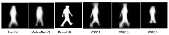
Figure 6.
Mask detection of the image FudanPed00035.png with different Mask R-CNN models, where the gamma value () is one.
The Mask R-CNN model detects objects by predicting bounding boxes, which can result in uncertainties due to the process of segmentation prediction, where the images are decomposed to pixels, the number of which is proportional to the size of the instance.
In the figure above, AP parameter indicates the average precision [11,20,26], and AR represents the average recall for both bounding boxes and segmentation. Accordingly, average precision defines how accurate the prediction is. On the contrary, average recall defines how well identified the proper classes are. The table below (see Table 4) shows that Mask R-CNN with the ResNet 50 backbone has the highest AP and AR value compared to the other models because it uses the residual network with a deeper layer. In other words, it contains 17 residual blocks.
Table 4.
Values of Average Precision and Average Recall for both bounding boxes and segmentation tabulated while using different backbones (the maximum values of the columns are denoted with *).
At the same time, VGG16 takes the longest time to train the model. Moreover, ResNet needs 0.003 s to evaluate it (see Table 5).
Table 5.
Training time and evaluating times are calculated for different backbones (the minimum values of the columns are denoted with *).
9. Evaluation
In this section, we introduce the evaluation of the investigated networks by processing 10 images with different gamma values. Images are indicated in the tables below with numbers from 0 to 9. We use score values to compare the different networks to indicate the probability of the proper classification. Their score value is shown in the contingency tables. Besides this, the bottom row contains the average score value related to the different images.
Mask R-CNN with AlexNet Backbone.
Table 6.
Top score of the 10 images represented by numbers 0 to 9 with different gamma values () while using Mask R-CNN with backbone Alex Net.
Table 6.
Top score of the 10 images represented by numbers 0 to 9 with different gamma values () while using Mask R-CNN with backbone Alex Net.
| Top Score Value | ||||||||
|---|---|---|---|---|---|---|---|---|
| Test Images | 0.1 | 0.2 | 0.3 | 0.4 | 0.5 | 1 | 1.5 | |
| 0 | 0.1092 | 0.0587 | 0 | 0.0648 | 0.1715 | 0.5374 | 0.1118 | |
| 1 | 0.0854 | 0 | 0 | 0.0685 | 0.158 | 0.5369 | 0.069 | |
| 2 | 0.1225 | 0.0594 | 0.0603 | 0.0698 | 0.1518 | 0.5276 | 0.0852 | |
| 3 | 0.1541 | 0.0917 | 0 | 0.0731 | 0.1479 | 0.5605 | 0.1314 | |
| 4 | 0.1415 | 0.0585 | 0.0639 | 0.0824 | 0.1341 | 0.5486 | 0.0953 | |
| 5 | 0.1737 | 0.121 | 0 | 0.0913 | 0.1385 | 0.5462 | 0.0887 | |
| 6 | 0.1359 | 0.08 | 0.0624 | 0.0841 | 0.1049 | 0.5342 | 0.1157 | |
| 7 | 0.1526 | 0.0743 | 0 | 0.0525 | 0.1144 | 0.5403 | 0.1174 | |
| 8 | 0.1327 | 0.0533 | 0.0509 | 0.0872 | 0.1341 | 0.5252 | 0.0732 | |
| 9 | 0.1198 | 0 | 0 | 0.0851 | 0.178 | 0.5135 | 0.1021 | |
| Average | 0.13274 | 0.05969 | 0.02375 | 0.07588 | 0.14332 | 0.53704 | 0.09898 | |
Mask R-CNN with MobileNet V2 Backbone.
Table 7.
Top score of the 10 images with different gamma values () while using Mask R-CNN with backbone Mobile Net V2.
Table 7.
Top score of the 10 images with different gamma values () while using Mask R-CNN with backbone Mobile Net V2.
| Top Score Value | ||||||||
|---|---|---|---|---|---|---|---|---|
| Test Images | 0.1 | 0.2 | 0.3 | 0.4 | 0.5 | 1 | 1.5 | |
| 0 | 0.1037 | 0.0935 | 0.0874 | 0.0826 | 0.122 | 0.4899 | 0.1032 | |
| 1 | 0.1021 | 0 | 0 | 0 | 0.0781 | 0.6261 | 0.0756 | |
| 2 | 0.109 | 0.0975 | 0.0661 | 0.0771 | 0.1038 | 0.6609 | 0.1351 | |
| 3 | 0.114 | 0.0896 | 0.0813 | 0.077 | 0.1073 | 0.6643 | 0.1171 | |
| 4 | 0.1365 | 0.112 | 0.0945 | 0.0606 | 0.1363 | 0.6215 | 0.0946 | |
| 5 | 0.1389 | 0.1277 | 0.059 | 0.0858 | 0.1089 | 0.6422 | 0.0807 | |
| 6 | 0.0878 | 0.0907 | 0.0746 | 0.0616 | 0.0927 | 0.6987 | 0.0856 | |
| 7 | 0.0985 | 0.0954 | 0.0774 | 0.0676 | 0.1007 | 0.6773 | 0.1011 | |
| 8 | 0.1076 | 0.1087 | 0.0947 | 0.0699 | 0.127 | 0.6693 | 0.1194 | |
| 9 | 0.1045 | 0.0549 | 0.0725 | 0.071 | 0.0851 | 0.5985 | 0.0569 | |
| Average | 0.11026 | 0.087 | 0.07075 | 0.06532 | 0.10619 | 0.63487 | 0.09693 | |
Mask R-CNN with ResNet50 Backbone.
Table 8.
Top score of the 10 images with different gamma values () while using Mask R-CNN with backbone ResNet 50.
Table 8.
Top score of the 10 images with different gamma values () while using Mask R-CNN with backbone ResNet 50.
| Top Score Value | ||||||||
|---|---|---|---|---|---|---|---|---|
| Test Images | 0.1 | 0.2 | 0.3 | 0.4 | 0.5 | 1 | 1.5 | |
| 0 | 0.677 | 0.8755 | 0.8625 | 0.8822 | 0.8686 | 0.9988 | 0.88 | |
| 1 | 0.6161 | 0.9058 | 0.9036 | 0.9032 | 0.9071 | 0.9976 | 0.92 | |
| 2 | 0.6315 | 0.8889 | 0.88 | 0.8846 | 0.8716 | 0.9958 | 0.895 | |
| 3 | 0.6486 | 0.8687 | 0.8721 | 0.8778 | 0.8729 | 0.9966 | 0.8862 | |
| 4 | 0.613 | 0.8566 | 0.8305 | 0.8427 | 0.8383 | 0.9967 | 0.8588 | |
| 5 | 0.6082 | 0.8319 | 0.8023 | 0.7977 | 0.7933 | 0.9904 | 0.8418 | |
| 6 | 0.6438 | 0.8465 | 0.8541 | 0.8556 | 0.856 | 0.9972 | 0.8872 | |
| 7 | 0.6061 | 0.8737 | 0.8579 | 0.8532 | 0.8507 | 0.9982 | 0.8841 | |
| 8 | 0.5955 | 0.8308 | 0.8229 | 0.8121 | 0.8116 | 0.998 | 0.8189 | |
| 9 | 0.5269 | 0.8534 | 0.8821 | 0.8685 | 0.866 | 0.9985 | 0.8851 | |
| Average | 0.61667 | 0.86318 | 0.8568 | 0.85776 | 0.85361 | 0.99678 | 0.87571 | |
Mask R-CNN with VGG11 Backbone.
Table 9.
Top score of the 10 images with different gamma values () while using Mask R-CNN with backbone VGG11.
Table 9.
Top score of the 10 images with different gamma values () while using Mask R-CNN with backbone VGG11.
| Top Score Value | ||||||||
|---|---|---|---|---|---|---|---|---|
| Test Images | 0.1 | 0.2 | 0.3 | 0.4 | 0.5 | 1 | 1.5 | |
| 0 | 0.1889 | 0.1629 | 0.1914 | 0.1337 | 0.1733 | 0.7792 | 0.175 | |
| 1 | 0.0851 | 0.0993 | 0.086 | 0.1407 | 0.1965 | 0.8253 | 0.1482 | |
| 2 | 0.2229 | 0.1983 | 0.2062 | 0.133 | 0.2092 | 0.7748 | 0.1773 | |
| 3 | 0.2128 | 0.2215 | 0.2034 | 0.1219 | 0.2051 | 0.7706 | 0.1749 | |
| 4 | 0.1816 | 0.1708 | 0.1674 | 0.1421 | 0.2152 | 0.75 | 0.1775 | |
| 5 | 0.2326 | 0.231 | 0.2264 | 0.1227 | 0.1889 | 0.7653 | 0.1853 | |
| 6 | 0.1875 | 0.2072 | 0.1849 | 0.1176 | 0.1843 | 0.819 | 0.1767 | |
| 7 | 0.2115 | 0.1955 | 0.1959 | 0.139 | 0.1741 | 0.7952 | 0.1643 | |
| 8 | 0.2199 | 0.1863 | 0.2001 | 0.1452 | 0.2207 | 0.7579 | 0.1791 | |
| 9 | 0.1191 | 0.1097 | 0.1057 | 0.1298 | 0.1668 | 0.5576 | 0.2018 | |
| Average | 0.18619 | 0.17825 | 0.17674 | 0.13257 | 0.19341 | 0.75949 | 0.17601 | |
Mask R-CNN with VGG13 Backbone.
Table 10.
Top score of the 10 images with different gamma values (γ) while using Mask R-CNN with backbone VGG13.
Table 10.
Top score of the 10 images with different gamma values (γ) while using Mask R-CNN with backbone VGG13.
| Top Score Value | ||||||||
|---|---|---|---|---|---|---|---|---|
| Test Images | 0.1 | 0.2 | 0.3 | 0.4 | 0.5 | 1 | 1.5 | |
| 0 | 0.0706 | 0.1952 | 0.1302 | 0.165 | 0.1275 | 0.7111 | 0.1958 | |
| 1 | 0.0685 | 0.08 | 0.1694 | 0.1439 | 0.1375 | 0.7227 | 0.1742 | |
| 2 | 0.0671 | 0.1873 | 0.1622 | 0.1585 | 0.1297 | 0.7334 | 0.2018 | |
| 3 | 0.064 | 0.1768 | 0.14 | 0.1602 | 0.1176 | 0.7446 | 0.2033 | |
| 4 | 0.0703 | 0.1739 | 0.1605 | 0.1666 | 0.1199 | 0.6729 | 0.2156 | |
| 5 | 0.0854 | 0.1767 | 0.1481 | 0.1617 | 0.1222 | 0.7071 | 0.193 | |
| 6 | 0.1682 | 0.1718 | 0.1436 | 0.1728 | 0.1383 | 0.7209 | 0.2092 | |
| 7 | 0.0644 | 0.1727 | 0.1269 | 0.1692 | 0.1232 | 0.7559 | 0.2012 | |
| 8 | 0.0714 | 0.18 | 0.1202 | 0.1314 | 0.1218 | 0.7607 | 0.2041 | |
| 9 | 0.0676 | 0.0995 | 0.1205 | 0.1205 | 0.1181 | 0.688 | 0.2397 | |
| Average | 0.07975 | 0.16139 | 0.14216 | 0.15498 | 0.12558 | 0.72173 | 0.20379 | |
Mask R-CNN with VGG16 Backbone.
Table 11.
Top score of the 10 images with different gamma values () while using Mask R-CNN with backbone VGG16.
Table 11.
Top score of the 10 images with different gamma values () while using Mask R-CNN with backbone VGG16.
| Top Score Value | ||||||||
|---|---|---|---|---|---|---|---|---|
| Test Images | 0.1 | 0.2 | 0.3 | 0.4 | 0.5 | 1 | 1.5 | |
| 0 | 0.0962 | 0.0939 | 0.0966 | 0.1385 | 0.0848 | 0.5924 | 0.1109 | |
| 1 | 0.0922 | 0.0702 | 0.0851 | 0.1592 | 0.114 | 0.588 | 0.109 | |
| 2 | 0.0976 | 0.0807 | 0.0973 | 0.1341 | 0.0857 | 0.5485 | 0.1101 | |
| 3 | 0.0923 | 0.0792 | 0.0923 | 0.1414 | 0.0779 | 0.5059 | 0.1163 | |
| 4 | 0.0936 | 0.0792 | 0.0958 | 0.16 | 0.1059 | 0.5174 | 0.114 | |
| 5 | 0.0986 | 0.1023 | 0.0995 | 0.1493 | 0.1453 | 0.5552 | 0.1186 | |
| 6 | 0.0891 | 0.1008 | 0.0953 | 0.1225 | 0.0978 | 0.5839 | 0.1133 | |
| 7 | 0.0988 | 0.0841 | 0.0939 | 0.145 | 0.0757 | 0.5848 | 0.1193 | |
| 8 | 0.0922 | 0.08 | 0.0998 | 0.1355 | 0.0792 | 0.5436 | 0.1232 | |
| 9 | 0.0903 | 0.0732 | 0.0885 | 0.1583 | 0.0941 | 0.5375 | 0.1146 | |
| Average | 0.09409 | 0.08436 | 0.09441 | 0.14438 | 0.09604 | 0.55572 | 0.11493 | |
As shown in the heat map below, Mask R-CNN with Resnet 50 had the best performance in all scenarios. If the gamma was 1, the average score value was 99.68%.
As the intensity of the image changes from dark to bright section, the scores of the ResNet increases until gamma 1. Generally, ResNet50 based Mask R-CNN model performs well in all scenarios. Even if the images become brighter, the score of the ResNet 50 decreases much slower than the other models (see Table 12).
Table 12.
Heat map of the Mask R-CNN models with respect to different values of gamma (). The colour of the cells changes from green to red, where green indicates high values and red indicates low values.
In our study, we tested the models on a custom dataset. However, in real life, the system must deal with real-time datasets. Accordingly, in the future, we are planning to test the KITTI dataset. It contains 3D data involving Lidar sensor data, images, etc.
We found a robust and flexible detection model (Mask R-CNN) that can perform well in any scenario, whether it is day or night. In future research steps, we are going to investigate images from rainy and smoky conditions.
Furthermore, self-driving cars are expected to be equipped with high-resolution cameras recording gamma value as well. Following this, it seems reasonable to use the automatic gamma correction method to improve the efficiency of the instance detection process in different driving conditions.
10. Conclusions
In a nutshell, ResNet50-based mask R-CNN model performs well in all lighting conditions, whether it is bright or dark. Conversely, the total loss of this model is 16.17%. Summing up, it is found that ResNet50 based Mask R-CNN is better for real-time detection systems, because self-driving cars run on the road with real data that changes in milliseconds. Second, low qualities of images can be automatically corrected with the gamma correction method. However, a brighter environment can also be a challenging factor. In addition to this, many factors can significantly influence image quality, such as fog, rain, smoke, vehicle speed, etc. Thus, from the above results, ResNet-based Mask R-CNN model is robust, flexible, and can efficiently support the driving process in all driving conditions.
Author Contributions
Conceptualization, Á.T.; methodology, Á.T. and Z.S.; software, M.J.; validation, Á.T.; formal analysis, M.J.; investigation, M.J.; resources, Z.S.; data curation, M.J.; writing—original draft preparation, M.J.; writing—review and editing, Á.T.; visualization, M.J.; supervision, Á.T.; project administration, Á.T. and Z.S.; funding acquisition, Z.S. All authors have read and agreed to the published version of the manuscript.
Funding
The research presented in this paper was supported by the NRDI Office, Ministry of Innovation and Technology, Hungary, within the framework of the Autonomous Systems National Laboratory Programme, and the NRDI Fund based on the charter of bolster issued by the NRDI Office. The presented work was carried out within the MASPOV Project (KTI_KVIG_4-1_2021), which was implemented with support provided by the Government of Hungary in the context of the Innovative Mobility Program of KTI.
Institutional Review Board Statement
Not applicable.
Informed Consent Statement
Not applicable.
Data Availability Statement
To explore the environmental conditions, a pedestrian custom dataset based on Common Object in Context (COCO) was used [55,56,57].
Conflicts of Interest
The authors declare no conflict of interest. The funders had no role in the design of the study; in the collection, analyses, or interpretation of data; in the writing of the manuscript; or in the decision to publish the results.
References
- Borek, J.; Groelke, B.; Earnhardt, C.; Vermillion, C. Economic Optimal Control for Minimizing Fuel Consumption of Heavy-Duty Trucks in a Highway Environment. IEEE Trans. Control. Syst. Technol. 2019, 28, 1652–1664. [Google Scholar] [CrossRef]
- Torabi, S.; Bellone, M.; Wahde, M. Energy minimization for an electric bus using a genetic algorithm. Eur. Transp. Res. Rev. 2020, 12, 2. [Google Scholar] [CrossRef]
- Fényes, D.; Németh, B.; Gáspár, P. A Novel Data-Driven Modeling and Control Design Method for Autonomous Vehicles. Energies 2021, 14, 517. [Google Scholar] [CrossRef]
- Aymen, F.; Mahmoudi, C. A novel energy optimization approach for electrical vehicles in a smart city. Energies 2019, 12, 929. [Google Scholar] [CrossRef] [Green Version]
- Skrúcaný, T.; Kendra, M.; Stopka, O.; Milojević, S.; Figlus, T.; Csiszár, C. Impact of the electric mobility implementation on the greenhouse gases production in central European countries. Sustainability 2019, 11, 4948. [Google Scholar] [CrossRef] [Green Version]
- Csiszár, C.; Földes, D. System model for autonomous road freight transportation. Promet-Traffic Transp. 2018, 30, 93–103. [Google Scholar] [CrossRef] [Green Version]
- Lu, Q.; Tettamanti, T. Traffic Control Scheme for Social Optimum Traffic Assignment with Dynamic Route Pricing for Automated Vehicles. Period. Poly. Transp. Eng. 2021, 49, 301–307. [Google Scholar] [CrossRef]
- Li, Q.; He, T.; Fu, G. Judgment and optimization of video image recognition in obstacle detection in intelligent vehicle. Mech. Syst. Signal Process. 2020, 136, 106406. [Google Scholar] [CrossRef]
- Yang, L.; Liu, Z.; Wang, X.; Yu, X.; Wang, G.; Shen, L. Image-Based Visual Servo Tracking Control of a Ground Moving Target for a Fixed-Wing Unmanned Aerial Vehicle. J. Intell. Robot. Syst. 2021, 102, 81. [Google Scholar] [CrossRef]
- Junaid, A.B.; Konoiko, A.; Zweiri, Y.; Sahinkaya, M.N.; Seneviratne, L. Autonomous wireless self-charging for multi-rotor unmanned aerial vehicles. Energies 2017, 10, 803. [Google Scholar] [CrossRef]
- Lee, S.H.; Kim, B.J.; Lee, S.B. Study on Image Correction and Optimization of Mounting Positions of Dual Cameras for Vehicle Test. Energies 2021, 14, 4857. [Google Scholar] [CrossRef]
- Tschürtz, H.; Gerstinger, A. The Safety Dilemmas of Autonomous Driving. In Proceedings of the 2021 Zooming Innovation in Consumer Technologies Conference (ZINC), Novi Sad, Serbia, 26–27 May 2021; pp. 54–58. [Google Scholar]
- Zhao, Z.Q.; Zheng, P.; Xu, S.T.; Wu, X. Object Detection with Deep Learning: A Review. IEEE Trans. Neural Netw. Learn. Syst. 2019, 30, 3212–3232. [Google Scholar] [CrossRef] [PubMed] [Green Version]
- Kohli, P.; Chadha, A. Enabling pedestrian safety using computer vision techniques: A case study of the 2018 uber inc. self-driving car crash. Lect. Notes Netw. Syst. 2020, 69, 261–279. [Google Scholar] [CrossRef] [Green Version]
- Barba-Guaman, L.; Naranjo, J.E.; Ortiz, A. Deep learning framework for vehicle and pedestrian detection in rural roads on an embedded GPU. Electron 2020, 9, 589. [Google Scholar] [CrossRef] [Green Version]
- Simhambhatla, R.; Okiah, K.; Slater, R. Self-Driving Cars: Evaluation of Deep Learning Techniques for Object Detection in Different Driving Conditions. SMU Data Sci. Rev. 2019, 2, 23. [Google Scholar]
- Cao, C.; Wang, B.; Zhang, W.; Zeng, X.; Yan, X.; Feng, Z.; Liu, Y.; Wu, Z. An Improved Faster R-CNN for Small Object Detection. IEEE Access 2019, 7, 106838–106846. [Google Scholar] [CrossRef]
- Sandler, M.; Howard, A.; Zhu, M.; Zhmoginov, A.; Chen, L.C. MobileNetV2: Inverted Residuals and Linear Bottlenecks. In Proceedings of the IEEE Conference on Computer Vision and Pattern Recognition (CVPR), Salt Lake City, UT, USA, 18–23 June 2018; pp. 4510–4520. [Google Scholar] [CrossRef] [Green Version]
- Alganci, U.; Soydas, M.; Sertel, E. Comparative research on deep learning approaches for airplane detection from very high-resolution satellite images. Remote Sens. 2020, 12, 458. [Google Scholar] [CrossRef] [Green Version]
- Huang, R.; Pedoeem, J.; Chen, C. YOLO-LITE: A Real-Time Object Detection Algorithm Optimized for Non-GPU Computers. In Proceedings of the 2018 IEEE International Conference on Big Data, Seattle, WA, USA, 10–13 December 2018; pp. 2503–2510. [Google Scholar] [CrossRef] [Green Version]
- Redmon, J.; Farhadi, A. YOLO v.3. Tech Rep. 2018, pp. 1–6. Available online: https://pjreddie.com/media/files/papers/YOLOv3.pdf (accessed on 1 February 2021).
- Suhail, A.; Jayabalan, M.; Thiruchelvam, V. Convolutional neural network based object detection: A review. J. Crit. Rev. 2020, 7, 786–792. [Google Scholar] [CrossRef]
- Lokanath, M.; Kumar, K.S.; Keerthi, E.S. Accurate object classification and detection by faster-R-CNN. IOP Conf. Ser. Mater. Sci. Eng. 2017, 263, 052028. [Google Scholar] [CrossRef]
- Girshick, R. Fast R-CNN. In Proceedings of the 2015 International Conference on Computer Vision (ICCV), Santiago, Chile, 7–13 December 2015; pp. 1440–1448. [Google Scholar] [CrossRef]
- Almubarak, H.; Bazi, Y.; Alajlan, N. Two-stage mask-R-CNN approach for detecting and segmenting the optic nerve head, optic disc, and optic cup in fundus images. Appl. Sci. 2020, 10, 3833. [Google Scholar] [CrossRef]
- Mahmoud, A.S.; Mohamed, S.A.; El-Khoribi, R.A.; AbdelSalam, H.M. Object detection using adaptive mask R-CNN in optical remote sensing images. Int. J. Intell. Eng. Syst. 2020, 13, 65–76. [Google Scholar] [CrossRef]
- Rezvy, S.; Zebin, T.; Braden, B.; Pang, W.; Taylor, S.; Gao, X.W. Transfer learning for endoscopy disease detection and segmentation with Mask-RCNN benchmark architecture. In Proceedings of the 2nd International Workshop and Challenge on Computer Vision in Endoscopy, Iowa City, IA, USA, 3 April 2020; pp. 68–72. [Google Scholar]
- Wu, X.; Wen, S.; Xie, Y.A. Improvement of Mask-R-CNN Object Segmentation Algorithm; Springer International Publishing: New York, NY, USA, 2019; Volume 11740. [Google Scholar]
- Penn-Fudan Database for Pedestrian Detection and Segmentation. Available online: https://www.cis.upenn.edu/~jshi/ped_html/index.html (accessed on 1 February 2021).
- Tv, C.R.T.; Crt, T.; Intensity, L.; Voltage, C.; Lcd, T. How to Match the Color Brightness of Automotive TFT-LCD Panels. pp. 1–6. Available online: https://www.renesas.com/us/en/document/whp/how-match-color-brightness-automotive-tft-lcd-panels (accessed on 1 February 2021).
- Farid, H. Blind inverse gamma correction. IEEE Trans. Image Process. 2001, 10, 1428–1433. [Google Scholar] [CrossRef] [PubMed]
- DeArman, A. The Wild, Wild West: A Case Study of Self-Driving Vehicle Testing in Arizona. 2010. Available online: https://arizonalawreview.org/the-wild-wild-west-a-case-study-of-self-driving-vehicle-testing-in-arizona/ (accessed on 1 February 2021).
- Mikusova, M. Crash avoidance systems and collision safety devices for vehicle. In Proceedings of the MATEC Web of Conferences: Dynamics of Civil Engineering and Transport Structures and Wind Engineering—DYN-WIND’2017, Trstená, Slovak Republic, 21–25 May 2017; Volume 107, p. 00024. [Google Scholar]
- Ammirato, P.; Berg, A.C. A Mask-R-CNN Baseline for Probabilistic Object Detection. 2019. Available online: http://arxiv.org/abs/1908.03621 (accessed on 1 February 2021).
- Zhang, Y.; Chu, J.; Leng, L.; Miao, J. Mask-refined R-CNN: A network for refining object details in instance segmentation. Sensors 2020, 20, 1010. [Google Scholar] [CrossRef] [Green Version]
- Michele, A.; Colin, V.; Santika, D.D. Mobilenet convolutional neural networks and support vector machines for palmprint recognition. Procedia Comput. Sci. 2019, 157, 110–117. [Google Scholar] [CrossRef]
- Sharma, V.; Mir, R.N. Saliency guided faster-R-CNN (SGFr-R-CNN) model for object detection and recognition. J. King Saud. Univ.-Comput. Inf. Sci. 2019. [Google Scholar] [CrossRef]
- Ren, S.; He, K.; Girshick, R.; Sun, J. Faster R-CNN: Towards Real-Time Object Detection with Region Proposal Networks. IEEE Trans. Pattern Anal. Mach. Intell. 2017, 39, 1137–1149. [Google Scholar] [CrossRef] [Green Version]
- Girshick, R.; Donahue, J.; Darrell, T.; Malik, J. Region-Based Convolutional Networks for Accurate Object Detection and Segmentation. IEEE Trans. Pattern Anal. Mach. Intell. 2016, 38, 142–158. [Google Scholar] [CrossRef] [PubMed]
- Özgenel, F.; Sorguç, A.G. Performance comparison of pretrained convolutional neural networks on crack detection in buildings. In Proceedings of the 35th International Symposium on Automation and Robotics in Construction (ISARC 2018), Berlin, Germany, 20–25 July 2018. [Google Scholar] [CrossRef]
- Iglovikov, V.; Seferbekov, S.; Buslaev, A.; Shvets, A. TernausNetV2: Fully convolutional network for instance segmentation. In Proceedings of the IEEE Conference on Computer Vision and Pattern Recognition (CVPR) Workshops, Salt Lake City, UT, USA, 18–23 June 2018; pp. 228–232. [Google Scholar] [CrossRef] [Green Version]
- Saha, R. Transfer Learning—A Comparative Analysis. December 2018. Available online: https://www.researchgate.net/publication/329786975_Transfer_Learning_-_A_Comparative_Analysis?channel=doi&linkId=5c1a9767299bf12be38bb098&showFulltext=true (accessed on 1 February 2021).
- Girshick, R.; Donahue, J.; Darrell, T.; Malik, J.; Berkeley, U.C.; Malik, J. Rich feature hierarchies for accurate object detection and semantic segmentation. In Proceedings of the IEEE Conference on Computer Vision and Pattern Recognition, Columbus, OH, USA, 23–28 June 2014; Volume 1, p. 5000. [Google Scholar] [CrossRef] [Green Version]
- Zhao, Y.; Han, R.; Rao, Y. A new feature pyramid network for object detection. In Proceedings of the 2019 International Conference on Virtual Reality and Intelligent Systems (ICVRIS), Jishou, China, 14–15 September 2019; pp. 428–431. [Google Scholar] [CrossRef]
- Krizhevsky, A.; Sutskever, I.; Hinton, G.E. ImageNet Classification with Deep Convolutional Neural Networks. Commun. ACM 2017, 60, 84–90. [Google Scholar] [CrossRef]
- Martin, C.H.; Mahoney, M.W. Traditional and heavy tailed self regularization in neural network models. In Proceedings of the 36th International Conference on Machine Learning, Long Beach, CA, USA, 9–15 June 2019; pp. 7563–7572. [Google Scholar]
- Alom, M.Z.; Taha, T.M.; Yakopcic, C.; Westberg, S.; Sidike, P.; Nasrin, M.S.; Van Esesn, B.C.; Awwal, A.A.S.; Asari, V.K. The History Began from AlexNet: A Comprehensive Survey on Deep Learning Approaches. 2018. Available online: http://arxiv.org/abs/1803.01164 (accessed on 1 February 2021).
- Almisreb, A.A.; Jamil, N.; Din, N.M. Utilizing AlexNet Deep Transfer Learning for Ear Recognition. In Proceedings of the 2018 Fourth International Conference on Information Retrieval and Knowledge Management (CAMP), Kota Kinabalu, Malaysia, 26–28 March 2018; pp. 8–12. [Google Scholar] [CrossRef]
- Sudha, K.K.; Sujatha, P. A qualitative analysis of googlenet and alexnet for fabric defect detection. Int. J. Recent Technol. Eng. 2019, 8, 86–92. [Google Scholar]
- Howard, A.G.; Zhu, M.; Chen, B.; Kalenichenko, D.; Wang, W.; Weyand, T.; Andreetto, M.; Adam, H. MobileNets: Efficient Convolutional Neural Networks for Mobile Vision Applications. 2017. Available online: http://arxiv.org/abs/1704.04861 (accessed on 1 February 2021).
- Reddy, A.S.B.; Juliet, D.S. Transfer learning with RESNET-50 for malaria cell-image classification. In Proceedings of the 2019 International Conference on Communication and Signal Processing (ICCSP), Chennai, India, 4–6 April 2019; pp. 945–949. [Google Scholar] [CrossRef]
- Rezende, E.; Ruppert, G.; Carvalho, T.; Ramos, F.; de Geus, P. Malicious software classification using transfer learning of ResNet-50 deep neural network. In Proceedings of the 2017 16th IEEE International Conference on Machine Learning and Applications (ICMLA), Cancun, Mexico, 18–21 December 2017; pp. 1011–1014. [Google Scholar] [CrossRef]
- Mikami, H.; Suganuma, H.; U-chupala, P.; Tanaka, Y.; Kageyama, Y. ImageNet/ResNet-50 Training in 224 Seconds, No. Table 2. 2018. Available online: http://arxiv.org/abs/1811.05233 (accessed on 1 February 2021).
- Simonyan, K.; Zisserman, A. Very deep convolutional networks for large-scale image recognition. In Proceedings of the 2014 International Conference on Learning Representations, Banff, AB, Canada, 14–16 April 2014; pp. 1–14. [Google Scholar]
- Rostianingsih, S.; Setiawan, A.; Halim, C.I. COCO (Creating Common Object in Context) Dataset for Chemistry Apparatus. Procedia Comput. Sci. 2020, 171, 2445–2452. [Google Scholar] [CrossRef]
- Lin, T.Y.; Maire, M.; Belongie, S.; Hays, J.; Perona, P.; Ramanan, D.; Dollár, P.; Zitnick, C.L. Microsoft COCO: Common Objects in Context. In Computer Vision—ECCV 2014; Fleet, D., Pajdla, T., Schiele, B., Tuytelaars, T., Eds.; Springer: Cham, Switzerland, 2017; Volume 8693, pp. 740–755. [Google Scholar] [CrossRef] [Green Version]
- Everingham, M.; van Gool, L.; Williams, C.K.I.; Winn, J.; Zisserman, A. The pascal visual object classes (VOC) challenge. Int. J. Comput. Vis. 2010, 88, 303–338. [Google Scholar] [CrossRef] [Green Version]
- Python Deep Learning Cookbook. Available online: https://livrosdeamor.com.br/documents/python-deep-learning-cookbook-indra-den-bakker-5c8c74d0a1136 (accessed on 1 February 2021).
- Guan, Q.; Wang, Y.; Ping, B.; Li, D.; Du, J.; Qin, Y.; Lu, H.; Wan, X.; Xiang, J. Deep convolutional neural network VGG-16 model for differential diagnosing of papillary thyroid carcinomas in cytological images: A pilot study. J. Cancer 2019, 10, 4876–4882. [Google Scholar] [CrossRef] [PubMed]
- Tammina, S. Transfer learning using VGG-16 with Deep Convolutional Neural Network for Classifying Images. Int. J. Sci. Res. Publ. 2019, 9, 9420. [Google Scholar] [CrossRef]
- Veit, A.; Matera, T.; Neumann, L.; Matas, J.; Belongie, S. COCO-Text: Dataset and Benchmark for Text Detection and Recognition in Natural Images. September 2016. Available online: http://arxiv.org/abs/1601.07140 (accessed on 1 February 2021).
- Mahamdioua, M.; Benmohammed, M. New Mean-Variance Gamma Method for Automatic Gamma Correction. Int. J. Image Graph. Signal Process. 2017, 9, 41–54. [Google Scholar] [CrossRef] [Green Version]
- Jin, L.; Chen, Z.; Tu, Z. Object Detection Free Instance Segmentation with Labeling Transformations. 2016, p. 1. Available online: http://arxiv.org/abs/1611.08991 (accessed on 1 February 2021).


Publisher’s Note: MDPI stays neutral with regard to jurisdictional claims in published maps and institutional affiliations. |
© 2021 by the authors. Licensee MDPI, Basel, Switzerland. This article is an open access article distributed under the terms and conditions of the Creative Commons Attribution (CC BY) license (https://creativecommons.org/licenses/by/4.0/).