A GRASP Approach for Solving Large-Scale Electric Bus Scheduling Problems

Abstract

Electrifying public bus transportation is a critical step in reaching net-zero goals. In this paper, the focus is on the problem of optimal scheduling of an electric bus (EB) fleet to cover a public transport timetable. The problem is modelled using a mixed integer program (MIP) in which the charging time of an EB is pertinent to the battery’s state-of-charge level. To be able to solve large problem instances corresponding to real-world applications of the model, a metaheuristic approach is investigated. To be more precise, a greedy randomized adaptive search procedure (GRASP) algorithm is developed and its performance is evaluated against optimal solutions acquired using the MIP. The GRASP algorithm is used for case studies on several public transport systems having various properties and sizes. The analysis focuses on the relation between EB ranges (battery capacity) and required charging rates (in kW) on the size of the fleet needed to cover a public transport timetable. The results of the conducted computational experiments indicate that an increase in infrastructure investment through high speed chargers can significantly decrease the size of the necessary fleets. The results also show that high speed chargers have a more significant impact than an increase in battery sizes of the EBs.

1. Introduction

In recent years there has been a staggering increase in the use of electric vehicles (EVs) on a global scale. Many governments have provided significant incentives for EV adoption to meet net-zero emission goals. One part of EV adoption is connected to the use of motorised individual transport that represents nearly one-third of the global carbon emissions [1]. A wide range of research is dedicated to optimizing their use through developing charging infrastructure and exploiting the potential of charging flexibility of EVs to solve problems related to the increased use of renewable energy production as discussed in [2,3,4].

The use of electric buses (EBs or eBuses) in public transport has been more prolific than personal transport vehicles. For example, in China there are currently more than 400,000 EVs in use. This corresponds to more than 14% of all buses in public transport in this country. An analysis on the expansion of EBs in China, through a case study regarding Beijing, can be found in [5]. The use of EBs offers a multitude of advantages such as decreased air and noise pollution within metropolitan areas. Another reason is that EBs are essential to reach net-zero goals and the adoption of EBs offers an economically viable public transportation when compared to diesel buses [6,7,8,9]. This is partly due to the high daily mileage of EBs. This results in a significant decrease in operational cost, due to the use of electricity instead of diesel, which quickly manages to cover the initial capital investment. For the same reason, a high penetration of EVs can be observed within car hailing and taxi services. In parallel, there is a growing research interest on the efficient planning of charging infrastructure for large fleets and exploiting smart charging scheduling in such systems [10,11,12,13].

The use of EBs introduces new operational challenges related to limited driving range and long charging times in comparison to diesel buses (DBs). The use of DBs in urban public transport is well represented using the vehicle scheduling problem (VSP) [14,15]. In the VSP, the goal is to optimize the assignment of a set of scheduled trips to a set of vehicles, where each trip is associated with one vehicle, based on some cost function frequently related to the number of used buses. This problem becomes significantly harder to solve in case of EBs due to additional constraints related to the range and the scheduling of the charging. These new issues are frequently modeled using the electric vehicle scheduling problem (E-VSP) [16] and its variations. It should be noted that even before the expanded use of EBs, the VSP has been considered with range constraints [17,18,19]. A recent survey can be found in [20]. We should note in passing that beyond vehicle scheduling there is a wealth of research dealing with public transport network design. Background regarding related models and research can be found in the following surveys [21,22].

Due to the growing amount of interest in the use of EBs, different approaches have been developed to address related practical problems. One part of this research is dedicated to charging infrastructure [23,24], while another direction is the analysis of operational issues. In [25,26], the long-term use of EBs is analyzed regarding scheduling and battery degradation. It should be noted that the infrastructural and operational aspects are closely connected and have been jointly considered [27,28] resulting in highly complex models. The scheduling of the use of EBs within a public transport system is well represented using the E-VSP and variations. Some of these variations are similar to the ones for the VSP, like the use of single [29,30,31,32] and multiple depots [33,34]. This problem has been considered from the point of pure EB [29,30,31] and mixed fleets [32,33]. A very interesting analysis of the problem of interest is given in [29], where the robustness is considered in relation to traffic conditions. In some variations, constraints related to the amount of charging that can be provided at a single time period have also been considered [29,32]. The majority of these models have been solved using mixed integer programs [29,30,31,32]. Only limited work has been done on the use of heuristic methods; some examples are the use of a combination of a greedy algorithm and simulated annealing [32] as well as the use of a genetic algorithm in [33].

The developed models and corresponding optimization methods are frequently used to evaluate the use of the EBs on relatively small systems. In the general case, only a few lines of a public transport system are analyzed, which is to a large extent a consequence of the high computational cost of solving the related MIPs. In this paper, the main objective is to provide a method that can be used to analyze the use of EBs on a large scale to cover a full public transport timetable. To achieve this, a greedy randomized adaptive search procedure (GRASP) [35] is developed for solving a variation of the single-depot E-VSP. In the proposed model, the charging time depends on the battery state. With the intention of lowering the complexity of the model, the following assumptions are made: charging is only allowed at the depot and there is no limit in the charging capacity. For the proposed model, firstly a MIP is developed to evaluate the performance of the GRASP algorithm. This is achieved with the following two objectives: (i) to observe from what system size on it is reasonable to use a metaheuristic method and (ii) to be able to evaluate the quality of solutions of the GRASP.

The developed GRASP algorithm is used for case studies on the use of EBs for public transport based on several real-world cases (cities). One part of the evaluation is dedicated to the battery size of EBs in the fleet. The second part is focused on the use of different chargers at the depot whose power can range from 50 kW to 600 kW. The conducted computational experiments are used to observe the size of the fleet needed to cover a public transport timetable for different battery sizes and charger types.

The main contributions of the conducted research are the following. Firstly, a new metaheuristic method is developed that extends the limited research on their application to eBus scheduling problems. The proposed GRASP algorithm manages to find high quality solutions for problem instances of larger size than previously developed methods. The second important contribution is related to the analysis of real-world public transport systems. To be more specific, the conducted case studies provide valuable insights on the use of eBuses with different ranges and charging infrastructure. In addition, the effect of different weather conditions, observed through different levels of energy consumption, on the variation in the size of eBus fleets needed to achieve a public transport timetable over the year is also analyzed.

The paper is organized as follows. The next section provides an outline of the model. The third section gives details of the graph formulation of the base problem. In the fourth section the MIP model is presented. Section 5 introduces the proposed GRASP algorithm. In Section 6, we present the results of the conducted computational experiments with a focus on some case studies for several cities. The paper ends with concluding remarks.

2. Model Outline

In this section, an outline of the proposed model is presented. The goal of the model is to find the minimal number of EBs that can cover all the bus lines in a timetable. More precisely, this is done by assigning a set of trips (timetable) to a set of EBs. A trip is specified with its origin, destination, duration, and starting time. The proposed model uses the following assumptions. The scheduling (assignment of EBs to trips) is done for a fixed time window, over a set of stations, and in a single depot. Moreover, the distances between all stations and the depot are assumed to be known in advance and recharging can only be done at the depot.

All trips are specified only by using origin and destination pairs and no intermediate stops are considered. It is assumed that all the buses start and end the day at the depot. An EB has a fixed driving range and a battery that must be recharged before the start of its schedule. Therefore, an EB can only be used if there is sufficient energy stored in its battery. It is assumed that all EBs move at a constant speed, so it is possible to use a scaling between length and duration. This is done with the goal of simplifying the calculation of the battery usage which will be proportional to the duration of a trip.

For an EB to be able to perform a trip from some origin, it has to be there before the starting time. The goal of the proposed model is to compare the number of needed EBs (having different ranges) and DBs to complete a public transport timetable. To that end, for a given timetable let us specify the specifics of the model as follows.

• There are N locations and the corresponding set of locations is represented by set $\mathcal{L}=\{1,\cdots ,N\}$.
• There is a single depot $D\in \mathcal{L}$.
• The distance between any two locations $i,j\in \mathcal{L}$ is known and is equal to $d_{ij}$.
• The schedule is done over P time periods and a corresponding set of time periods is denoted by $\mathcal{P}=\{1,\cdots ,P\}$.
• A timetable trip is a 4-tuple $\{o,d,s,l\}$, where origin-destination pairs are in the set of existing locations, that is, $\{o,d\}\subset \mathcal{L}$ and other parameters are part of time periods, that is $\{s,l\}\subset \mathcal{P}$. The timetable is a set $\mathcal{T}$ of timetable trips. For simplicity of notation, we will use $e=s+l$ for each trip to indicate the time of its completion.
• An EB has a battery capacity that provides a fixed range R. It is assumed that all EBs have the same range.
• The objective is to find the minimal number of EBs that can perform all the trips in the timetable.
• An EB can only be charged at a depot.
• An EB is fully charged at the first time period.
• There is a charging rate $\gamma$, i.e., how much a battery is charged in one time period.
• Charging of an EB is always done to full capacity.

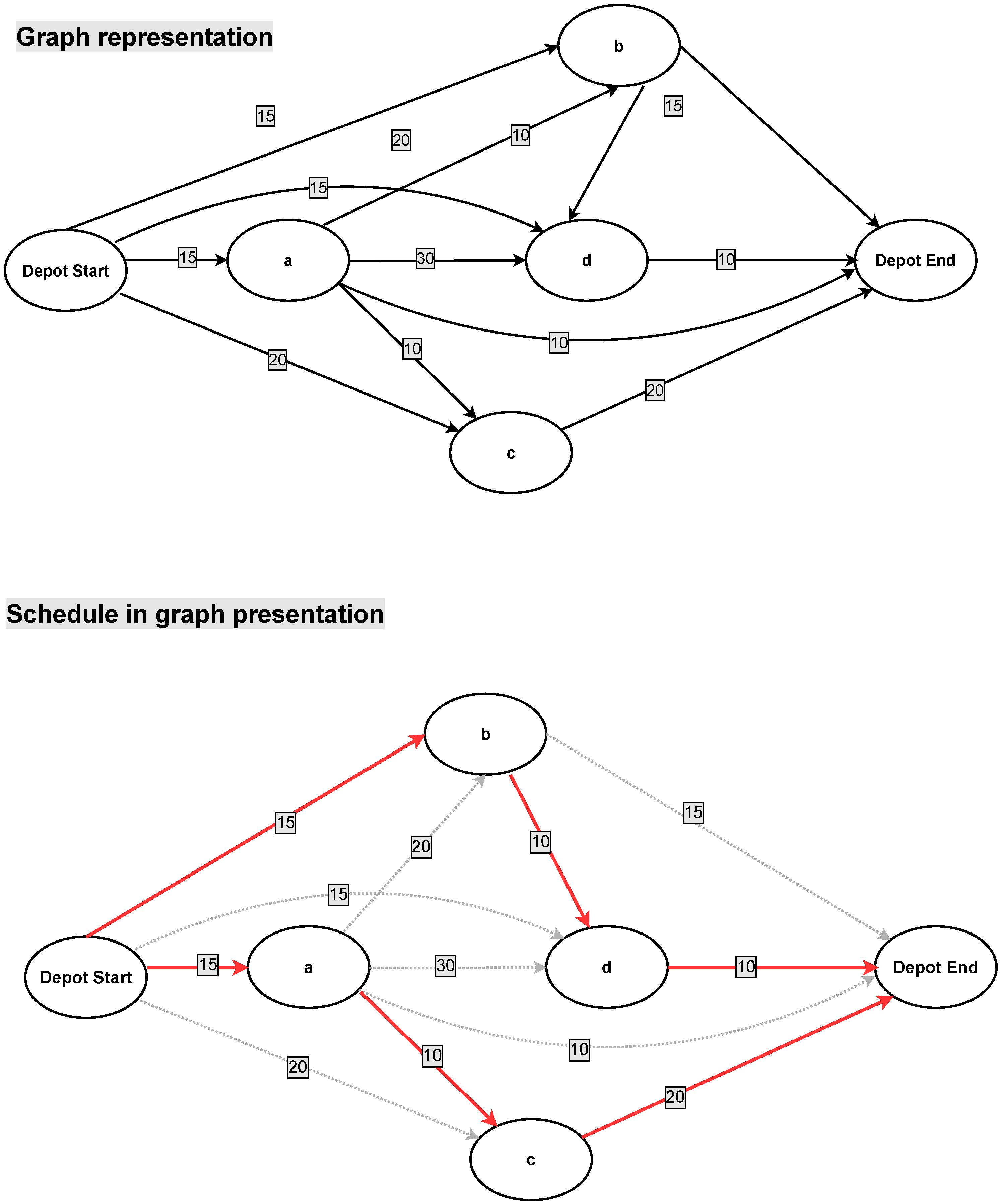
3. Graph Formulation

In this section, the graph formulation for the scheduling of buses is given. The basic idea of the graph formulation is similar to the one used in [29]. It only considers assignment of buses to trips in the timetable. In the later sections details on how this model is extended to include battery capacity and battery recharging are discussed more specifically.

Let us define a directed graph $G(V,E)$ to represent the problem. For each trip $t\in \mathcal{T}$ there is a node $t\in V$. In addition, the node set V contains two auxiliary nodes $D_s$ and $D_e$ as the start (departure from the depot) and the end (arrival to the depot) trip of all buses, respectively. In the following text, the notation $V_t$ will be used for the set of all nodes that correspond to timetable trips. Let us define the distance between two nodes (trips) i and j as the distance between the destination $i_d$ of trip i and origin $j_o$ of trip j as follows.

$$d_{ij}={\widehat{d}}_{i_d{j}_s}$$

(1)

An edge $(i,j)$ is a part of the edge set E if it is possible to perform trip j after trip i. Let us formally define the set of edges E in the following way.

$$\begin{array}{ccc}\hfill E_n& =& \{(i,j)\mid i,j\in \mathcal{L}\wedge (s_j-e_i-d_{ij}\ge 0)\}\hfill \end{array}$$

(2)

$$\begin{array}{ccc}\hfill E_s& =& \{(D_s,i)\mid i\in \mathcal{L}\}\hfill \end{array}$$

(3)

$$\begin{array}{ccc}\hfill E_e& =& \{(i,D_e)\mid i\in \mathcal{L}\}\hfill \end{array}$$

(4)

$$\begin{array}{ccc}\hfill E& =& E_n\cup E_s\cup E_e\hfill \end{array}$$

(5)

The set $E_n$ contains all the trip pairs $(i,j)$ such that the starting time of trip j ($s_j$) is greater or equal to the sum of the completion time $e_i$ of trip i and the travel time from the destination of trip i to the origin of trip j ($d_{ij}$). An edge connects the start-trip node $D_s$ to all other nodes ($E_s$). All the trip nodes are connected to the end node $D_e$. Finally, E is the set of all edges that exist in the graph. Note that, due to the definition of the edge set, the directed graph G does not contain any cycles. Each edge $(i,j)\in E$ has an additional property equal to its length.

The schedule for buses is presented as a directed graph $S(V,\tilde{E})$ which is a subgraph of G. An edge $(i,j)$ indicates that a bus performs trip j right after trip i. Let us make some observations about the solution defined in this way for the problem of interest. The set of vertices of graph S is the same as the one of G which means that all the trips are performed by some EB. Each trip node $i\in V_t$ will have exactly one incident edge for a node $x\in V$ of type $(i,x)$ since it can be performed directly before/after only one other trip. The number of edges having the form $(D_s,i)$ is equal to the number of buses needed to complete the timetable. Consequently, the schedule for a single bus will be a directed path having the form $(D_s,\cdots ,D_e)$. An illustration on how a trip timetable with known distances between locations and bus schedule is converted to the graph formulation can be seen in Figure 1.

4. Mathematical Model

In this section, based on the presented formulations, the mixed integer program for the problem of interest is presented. The proposed formulation has similarities to the ones given in [29,36]. The model uses the following input parameters:

• The distance between any two trips $i,j\in V$ is known and is equal to $d_{ij}$ which is calculated as described in the previous section.
• For each trip i there is a starting time $s_i$ and a duration $d_i$. For simplicity of notation, let us define $e_i=s_i+d_i$ as the time when trip i is completed.
• The charging rate per time period is denoted by $\gamma$.
• Battery usage per time period is denoted by $\alpha$.
• The battery capacity of all EBs is denoted by G.

The schedule of EBs and battery-related constraints are specified in the model using the following decision variables:

• For each $(i,j)\in E$ let us define a binary variable $x_{ij}$ which states whether some EB performs a trip j after i.
• For each trip $i\in V$ let us define $b_i$ as the state of the battery of the EB when it has arrived at the origin of trip i but before performing it.
• For each $i\in V$ let us define a binary variable $c_i$ which states whether the EB that performs trip i charges its battery after completing it.

The selected objective function of the model is to minimize the number of used EBs to complete all the trips in the timetable. As previously stated, the number of buses is equal to the number of edges starting from the start node $D_s$, which can be formally represented using the following formula:

$$\mathrm{Minimize}\sum _{i\in V_t}{x}_{D_{s}i}.$$

(6)

The last step in specifying the proposed model is defining its constraints. This is done in (9)–(20). The set of constraints can be divided into three groups. The first one, in (9)–(11), is dedicated to the completion of all the trips in the timetable by some EB. This set of constraints does not consider the range of EBs. The constraints (12)–(18) focus on the state of the battery and consequently on the range of the EBs. The constraints (19)–(20) are dedicated to the charging of EBs.

Parts of the battery-related constraints are conditional. For the sake of clarity, let us define two kinds of auxiliary variables, that are strictly specified by the values of $x_{ji}$ and $c_j$. In practice they are not necessary but increase the readability of the constraints. The first one is as follows:

$$v_{ji}=1-x_{ji}+c_j.$$

(7)

The variable $v_{ji}$ is used to recognize the state when an EB performs trip j before trip i and the EB is not charged after trip j. In this case the value of $v_{ji}$ is equal to 0. The second type of auxiliary variables is as follows:

$$w_{ji}=2-x_{ji}-c_j.$$

(8)

The variable $w_{ji}$ is used to recognize the state when an EB performs trip j before trip i and it is charged after trip j. In this case the value of $w_{ji}$ is equal to 0. Now, all the constraints of the proposed model can be defined as follows:

$$\begin{array}{ccc}\hfill \mathrm{(9)}& \hfill \sum _{(i,j)\in E}{x}_{ij}=1& & i\in V_t,\hfill \hfill \mathrm{(10)}& \hfill \sum _{(i,j)\in E}{x}_{ij}=1& & j\in V_t,\hfill \hfill \mathrm{(11)}& \hfill \sum _{i\in V_t}{x}_{D_{s}i}=\sum _{i\in V_t}{x}_{i{D}_e},& & \hfill \mathrm{(12)}& \hfill b_i-\alpha d_i\ge \alpha d_{i{D}_e}& & i\in V_t,\hfill \hfill \mathrm{(13)}& \hfill b_i\le M{v}_{ji}+b_j-\alpha (d_j+d_{ji})& & i\in V_t,j\in V,\hfill \hfill \mathrm{(14)}& \hfill b_i\ge -M{v}_{ji}+b_j-\alpha (d_j+d_{ji})& & i\in V_t,j\in V,\hfill \hfill \mathrm{(15)}& \hfill b_i\le M{w}_{ji}+G-\alpha d_{D_{s}i}& & i\in V_t,j\in V,\hfill \hfill \mathrm{(16)}& \hfill b_i\ge -M{w}_{ji}+G-\alpha d_{D_{s}i}& & i\in V_t,j\in V,\hfill \hfill \mathrm{(17)}& \hfill b_{D_s}=G,& & \hfill \mathrm{(18)}& \hfill b_i\le G& & i\in V_t,\hfill \hfill \mathrm{(19)}& \hfill s_i\ge -M{w}_{ji}& & \hfill +e_j+d_{j{D}_e}+d_{D_{s}i}& & \\ \hfill +\frac{1}{\gamma }(G-(b_i-d_i-d_{i{D}_e}))& & i,j\in V_t,\hfill \\ \hfill \mathrm{(20)}& \hfill 0\le c_j\le 1& & j\in V_t.\hfill \end{array}$$

The constraints in Equations (9) and (10) guarantee that only one trip is performed by an EB after and before a timetable trip i, respectively. Note that the starting at the depot and finalizing the day at the depot are also considered as trips (pull-out and pull-in). The constraint in Equation (11) states that there is an equal number of EBs that leave the starting depot and arrive at the ending depot.

The next set of constraints is related to the battery state of charge. Constraints given in (12) provide the minimal value of the battery load before a timetable trip i is performed. The battery value must be greater or equal to the charge needed to perform trip i and to reach the depot afterwards. The constraints in (13) and (14) are conditional ones implemented using a large value M. These constraints only have an effect if $v_{ji}=0$, or, in other words, if an EB performs trip i after trip j and does not charge between these trips. In this case, the state of the battery is equal to the state of the battery after trip j ($b_j$) minus the battery used for completing trip j and relocating to the origin of trip i. In a similar way, the constraints given in (15) and (16) are conditional constraints for the case if a bus is charged between trips j and i, specified in the variable $w_{ji}$. In this case the state of the battery charge before performing trip i is equal to the full battery (G) minus the charge needed to move from the depot to the origin of timetable trip i. It should be noted that a sufficiently high value of M for (13)–(16) is $2G$ (two times the EB battery capacity). The constraint in (17) guarantees that an EB leaves the starting depot with a full battery. The constraints given in (18) are used to enforce the battery capacity before the start of any timetable trip.

The conditional constraints given in (19) are used to specify when the battery can be charged between trips j and i. These constraints are related to time periods. To be more precise, charging between trips i and j can only be performed if after completing trip j, at time period $e_j$, there is enough time to move from the destination of trip j to the depot, move from the depot to the origin of trip i and charge the battery to its full capacity before the starting time of trip j ($s_j$). Note that a sufficient value for large M in this constraint is $2P$.

5. GRASP Algorithm

In practical real-world cases, the scheduling of EBs to achieve a public transport timetable generally requires solving large problem instances. As it will be seen in the results section, the use of the presented MIP is effective only for problem instances of limited size. Hence, a metaheuristic approach—a GRASP algorithm—is developed to achieve high quality solutions for large-scale problem instances. In this section, details of the proposed algorithm are presented. First, a simple greedy algorithm is introduced. Second, it is extended to a GRASP algorithm by adding a local search and randomization.

5.1. Greedy Algorithm

The basic idea of the proposed algorithm is to start with a schedule containing a minimal number of trips and gradually expanding it with new ones. In the implementation of this simple idea, a graph formulation is used. The solution has the form of a set of paths $\mathcal{P}=\{P_1,\cdots ,P_n\}$, each corresponding to an EB (path), as previously described. Let us use the notation $T\left(P\right)$ as the set of all timetable trips t such that $t\in P$. In addition let us define the same function for a set of paths (EBs) as

$$T\left(\mathcal{P}\right)=\bigcup _{P\in \mathcal{P}}T\left(P\right).$$

(21)

A set of paths $\mathcal{P}$ is a complete solution if it contains all the trips in the timetable, formally written as $\mathcal{T}\subset T\left(\mathcal{P}\right)$. To fully specify the greedy algorithm, we need to define the initial solution, a list of candidates and the heuristic function. The simplest initial partial solution can consist of a single path $P_0=\{D_s,D_e\}$. On the other hand, it is evident that there is a set U of trips that cannot be performed after any timetable trip, or, in other words, must be the first daily trip of an EB, which corresponds to the nodes that have no entering edges in the set $E_n$ but only in $E_s$. Using the set U, a larger initial solution, that has a path for each such trip, is defined as

$$\mathcal{P}=\{(D_s,t,D_e)\mid t\in U\}.$$

(22)

Note that for a partial solution $\mathcal{P}$, a trip t can only be added to at most one position in each path $P_i\in \mathcal{P}$. This is due to the fact that the starting/ending times of trips in $\mathcal{P}$ are strictly ascending. Consequently, a candidate for expansion will have the form $(t,P)$ where $t\in \mathcal{T}\setminus T\left(\mathcal{P}\right)$ is a trip, not already in the partial solution, and $P\in \mathcal{P}$ is a path (EB) in the partial solution. Note that it is possible to have a trip t that cannot be inserted to any of the paths $P\in \mathcal{P}$ in the current partial solution. Because of this fact, the set of paths, used to generate the candidates for the greedy algorithm, has an additional one that makes it possible to add new buses to the solution. This path will have the form $(D_s,D_e)$.

Let us analyze the valid candidates that are in the form of $(t,P)$. The term “valid" is used in the sense that the battery charge level of an EB has to be positive and less than the battery size during the entire schedule. To achieve this, let us define a function $B(P,i)$ as the state of the battery for a path P after i trips have been completed. Let us use the notation $p_i$ for the i-th timetable trip in path P. The function $B(P,i)$ is defined recursively as follows

$$\begin{array}{ccc}\hfill B(P,0)& =& G,\hfill \end{array}$$

(23)

$$\begin{array}{ccc}\hfill B(P,i)& =& \left\{\begin{array}{c}B(P,i-1)-\alpha (d_{p_{i-1}{p}_i}-d_{p_i})CanCharge(P,i)=\perp ,\hfill \\ G-\alpha (d_{D{p}_i}-d_{p_i})CanCharge(P,i)=\top .\hfill \end{array}\right.\hfill \end{array}$$

(24)

The equation given in (23) states that the initial (bus at depot) level of charge of the battery is equal to its capacity. Equation (24) is used to calculate the battery state after trip i. The notation ⊤ and ⊥ is used for the values true and false, respectively. It is assumed that if it is possible to charge the EB between trips $p_{i-1}$ and $p_i$ it will be charged. In this case the battery state after trip $p_i$ is equal to the full battery minus the battery usage needed to travel from the depot to the origin of trip $p_i$ and performing the trip $p_i$. In case the battery cannot be charged, this value is equal to the battery state after trip $p_{i-1}$ minus the battery used for moving from the destination of trip $p_{i-1}$ to the origin of trip $p_i$ and performing the trip $p_i$. Let us specify when the EB can be charged between $p_{i-1}$ and $p_i$, or, in other words, the function $CanCharge(P,i)$. This is done in the same way as in constraint (19) of the MIP formulation. For the sake of increasing the readability, the definition of the corresponding function is explicitly given in the following way:

$$\begin{array}{ccc}\hfill C^t(P,i)& =& \frac{B(P,i)-\alpha d_{p_{i}D}}{\gamma },\hfill \end{array}$$

(25)

$$\begin{array}{ccc}\hfill CanCharge(P,j)& \equiv & s_i-(e_{i-1}+d_{p_{i-1}D}+d_{D{p}_i}+C^t(P,i))\ge 0.\hfill \end{array}$$

(26)

The equation given in (25) defines the function that gives the time needed to charge the battery after the i-th trip of path P is completed and the bus has reached the depot. The charging time is inversely proportional to the charging rate $\gamma$. The equation given in (26) states that an EB can be charged between trips $p_{i-1}$ and $p_i$ if the starting time of trip $p_i$ ($s_{p_i}$) is after the earliest time trip $p_{i-1}$ can be completed ($e_{p_{i-1}}$) and the time the EB needs to move to the depot, and fully charge the battery and move from the depot to the origin of trip $p_i$.

Using the function $B(P,i)$, a Boolean function $valid\left(P\right)$ can be defined that states if a path is valid as follows

$$valid\left(P\right)\equiv \forall (i\in \{1,\cdots ,\left|P\right|\left\}\right)(B(P,i)\ge \alpha d_{p_{i}D}).$$

(27)

Equation (27) states that for each trip in a path, the charge of the battery is sufficient to arrive to the depot. Now, let us use the notation $P^{+t}$ as the path acquired by inserting trip t in path P. A candidate $(t,P)$ is valid if $valid\left(P^{+t}\right)$ is true.

The next step in defining the greedy algorithm is specifying the heuristic function. The idea of the heuristic function is to first avoid adding new paths (EBs) to the solution, unless necessary. The second part is to avoid unnecessary movements of EBs. Let us first define the length of additional movement of an EB, or more precisely for its path P, using the following formula:

$$\begin{array}{ccc}\hfill Move(P,i)& =& \left\{\begin{array}{c}{d}_{p_{i-1}{p}_i}CanCharge(P^{+t},i)=\perp \hfill \\ d_{p_{i-1}D}+d_{D{p}_i}CanCharge(P^{+t},i)=\top \hfill \end{array}\right.\hfill \end{array}$$

(28)

$$\begin{array}{ccc}\hfill Move\left(P\right)& =& \sum _{i=1..\left|P\right|}Move(P,i)\hfill \end{array}$$

(29)

In (28), the function $Move(P,i)$ is equal to the additional movement performed between trips $i-1$ and i of path P. The additional movement depends on the case if charging is performed or not between these two trips. The total additional movement for a path P is given in (29) with the function $Move\left(P\right)$ and is equal to the sum of additional movements for all consecutive trips.

Using function $Move$, the heuristic function h, for a valid expansion candidate $(P,t)$, can be specified as follows

$$\begin{array}{ccc}\hfill h(P,t)& =& \left\{\begin{array}{c}Move\left(P^{+t}\right)-Move\left(P\right)P\ne (D_s,D_e)\hfill \\ \\ h_n\left(t\right)P=(D_s,D_e)\hfill \end{array}\right.\hfill \end{array}$$

(30)

$$\begin{array}{ccc}\hfill h_n\left(t\right)& =& \left\{\begin{array}{c}M(\exists Q\in \mathcal{P})valid\left(Q^{+t}\right)\hfill \\ motherwise\hfill \end{array}.\right.\hfill \end{array}$$

(31)

The heuristic function $h(P,t)$, given in (30), differentiates between the cases when a new path is added or not. In case when no new path is added, the preference is for the smallest increase in the additional movement. In case when a new path is added, the heuristic function $h_n\left(t\right)$ is used and only depends on the trip t. In Equation (31), m and M are constants satisfying $m<<Move(P,t)<<M$ for any candidate $(P,t)$. The heuristic $h_n\left(t\right)$ states that in case a trip t can be added to some path $Q\in \mathcal{P}$ producing a valid path $Q^{+t}$, adding a new path $(D_s,t,D_e)$ to the solution is the least desirable. On the contrary, if the trip t cannot be added to any path $Q\in \mathcal{P}$ producing a valid one, then adding the path $(D_s,t,D_e)$ is most desirable. The reason for this is that if a path $Q^{+t}$ is not valid, it is not possible to expand Q to a path R in a way that $R^{+t}$ is a valid path. Therefore, it is preferable to add the new necessary path earlier to the solution. This is because in the later iterations of the greedy algorithm there will be a larger number of candidates for expansion, potentially of higher quality.

Using the heuristic function h, the greedy algorithm can be fully specified for which details can be seen in the pseudocode given in Algorithm 1. In this algorithm, the first stage is the generation of an initial solution $\mathcal{P}$ based on Equation (22). Next, the set of available trips ${\mathcal{T}}^c$ is set to all the trips in the timetable $\mathcal{T}$. In the main loop, at each iteration, firstly, the set of all valid candidates for expansion of the partial solution $\mathcal{C}$ is generated. Elements of $\mathcal{C}$ have the form $(P,t)$ where $P\in \mathcal{P}$ and $t\in {\mathcal{T}}^c$. Out of all $(P,t)\in \mathcal{C}$, the one having the minimal value of the heuristic function is selected for expanding the partial solution. Ties are randomly broken. This means that the timetable trip t is inserted in the path P. Further, notice that t can only be inserted at one unique place in path P based on its starting and ending times $s_t$ and $e_t$, respectively. Next, the trip t is removed from the set of available trips ${\mathcal{T}}^c$. The main loop is completed when all timetable trips are added to the solution $\mathcal{P}$, or, in other words, ${\mathcal{T}}^c$ is an empty set.

Algorithm 1 Greedy Algorithm

Generate initial solution $\mathcal{P}$ using Equation (22)

${\mathcal{T}}^c=\mathcal{T}\setminus T\left(\mathcal{P}\right)$

while${\mathcal{T}}^c\ne \varnothing$do

Generate set of valid candidates $\mathcal{C}$ for $\mathcal{P}$, ${\mathcal{T}}^c$

$(P,t)=argmi{n}_{(P,t)\in \mathcal{C}}h(P,t)$

Expand $\mathcal{P}$ with candidate $(P,t)$

${\mathcal{T}}^c={\mathcal{T}}^c\setminus \left\{t\right\}$

end while

5.2. GRASP Extension

In this section, details are provided on how the presented greedy algorithm is extended to the GRASP metaheuristic. To achieve this, the greedy algorithm needs to be randomized and a local search is added. In the proposed algorithm, the randomization is done using the standard restricted candidate list (RCL) approach. In case of an RCL with n elements, instead of selecting the candidate for expansion having the best value of the heuristic function, as in the deterministic greedy algorithm, one of the best n candidates is randomly selected.

The local search follows an approach commonly used in bin packing problems [37]. The idea is to check if the schedule has an EB such that all of its trips can be reassigned to other already used EBs. If this is possible, the procedure is repeated for the new schedule. The application of this simple concept is given in the following text. Firstly, the procedure on how the trips performed by one EB are relocated to the other ones is explained and later the complete local search.

The goal is to reassign one by one all the trips from one EB to the remaining ones. The pseudocode corresponding to the procedure of attempting the relocation of all the trips from the EB corresponding to path P to all the remaining EBs, a subset of the set of paths $\mathcal{P}$, is given in Algorithm 2. The function $RelocatePath$ returns a new set of paths $\mathcal{Q}$ if all the trips in path P can be relocated or an empty set if this is not possible.

Algorithm 2 Path Removal

functionRelocatePath($\mathcal{P}$, P)

$\mathcal{Q}=\mathcal{P}\setminus \left\{P\right\}$

Set R to all trips in P

while $R\ne \varnothing$ do

Select random $r\in R$

${\mathcal{Q}}_v=\{Q\mid (Q\in \mathcal{Q})\wedge valid\left(Q^{+r}\right)\}$

if ${\mathcal{Q}}_v=\varnothing \mathbf{then\; return} \varnothing$

end if

$Q_s=argmi{n}_{Q\in {\mathcal{Q}}_v}h(Q,r)$

$Q_s=Q_s^{+r}$

$R=R\setminus \left\{r\right\}$

end while

return $\mathcal{Q}$

end function

In this function, firstly, $\mathcal{Q}$ is set to the set of all paths in $\mathcal{P}$ except P. The set $\mathcal{Q}$ is used for creating the new schedule. Next, a set of trips R is set to all the trips that need to be relocated. The goal of the main loop is to relocate all the trips in R to other EBs one by one. At each iteration of the main loop, one of the trips $r\in R$ is selected randomly. For trip r, the set of valid candidates (EBs) for reassignment $Q_v$ is generated using the function $valid\left(Q^{+r}\right)$ for all the EBs $Q\in \mathcal{Q}$. In case ${\mathcal{Q}}_v$ is an empty set, the function $RelocatePath$ cannot reassign all the trips in path P, and the function returns an empty schedule.

Note that by randomizing the order in which the trips in the original path P are selected for reassignment increases the number of potential schedules that are explored in case the local search is applied to a same solution $\mathcal{P}$. The next step is selecting to which EB the trip r is reassigned from the set of all the valid ones ${\mathcal{Q}}_v$. This is done using the same heuristic h as in the case of the greedy algorithm. To be more precise, the trip r is reassigned to the EB, corresponding to the path $Q\in {\mathcal{Q}}_v$, that has the minimal value of $h(Q,r)$. The final step in the main loop is removing r from the set of trips R that need to be reassigned. The main loop is completed when all the trips have been reassigned or, in other words, when set R is empty.

Let us now define the complete local search using the function $RelocatePath$. The details of the local search can be seen in Algorithm 3. In this algorithm, the first step is setting the current best solution ${\mathcal{P}}^c$ to the schedule $\mathcal{P}$. The outer loop attempts to improve ${\mathcal{P}}_c$ when possible. This is achieved by setting the set of candidate paths for removal $\mathcal{Q}$ to all the paths in ${\mathcal{P}}_c$. The inner loop checks if any of the paths in $\mathcal{Q}$ can be removed from ${\mathcal{P}}^c$. This is done by selecting a random path $Q\in \mathcal{Q}$. Next, the function $Relocate({\mathcal{P}}^c,Q)$ checks if it is possible to remove the path Q. If this is true, the current best solution is updated, and the inner loop is exited. In case this is not true, the path Q is removed from the set of candidate paths $\mathcal{Q}$. This procedure is repeated until set $\mathcal{Q}$ is empty, or, in other words, it is not possible to further improve the solution ${\mathcal{P}}^c$.

Algorithm 3 Local Search

functionLocalSearch($\mathcal{P}$)

${\mathcal{P}}^c=\mathcal{P}$

repeat

$\mathcal{Q}={\mathcal{P}}^c$

while $\mathcal{Q}\ne \varnothing$ do

Select random $Q\in \mathcal{Q}$

if $RelocatePath({\mathcal{P}}^c,Q)\ne \varnothing$ then

${\mathcal{P}}^c=RelocatePath({\mathcal{P}}^c,Q)$

break

end if

$\mathcal{Q}=\mathcal{Q}\setminus \left\{Q\right\}$

end while

until No Improvement

end function

5.3. Implementation

In this subsection, the details of the proposed GRASP algorithm and its pseudocode are discussed and details are presented in Algorithm 4.

Algorithm 4 GRASP algorithm

$N=0$

while ($N\le MaxSolutions$) do

Generate solution $\mathcal{P}$ using $GreedyRCL\left(n\right)$

$\mathcal{P}=LocalSearch\left(\mathcal{P}\right)$

Check if $\mathcal{P}$ is new best solution

$N=N+1$

end while

The GRASP algorithm repeatedly generates new solutions $\mathcal{P}$ using function $GreedyRCL\left(n\right)$. This is done using the randomized version of the greedy algorithm given in Algorithm 1. In this algorithm, the heuristic function $h(P,t)$ is substituted with an RCL having n elements. On each such solution, the local search is applied and is checked if it is the new best solution. This procedure is repeated until a maximal number of solutions is generated or potentially some other stopping criterion is satisfied.

It is important to point out that in the practical implementation, it is not necessary to recalculate all the values of the heuristic function at every iteration. For instance, if at one iteration, it is impossible to add a trip to an EB it will remain to be so in all the later steps. The values of functions h, $CanCharge$, B only need to be recalculated at iteration $i+1$ for the paths that have been changed at iteration i. Exploiting this can significantly improve the computation performance of the method.

6. Results

In this section, the results of the conducted computational experiments are presented. The main goal is to provide a tool that can analyze the potential increase in the number of EBs needed to achieve a public transport timetable compared to the use of DBs. Because of this, the computational experiments have two objectives. The first one is to evaluate the effectiveness of the proposed MIP and GRASP for the newly proposed problem. The limits on the size of the problem instances that can be solved to optimality using the MIP within a reasonable time are found. The obtained solutions are, then, used to evaluate the performance of the proposed GRASP algorithm with respect to the quality of results. In addition, the computational cost of the GRASP algorithm is also analyzed. These tests have been conducted on synthetic problem instances.

In the final experiments, the GRASP algorithm is used to address practical issues related to the use of EBs in public transport. This is done through case studies on several real-world cities and corresponding public transport timetables. Moreover, the relation between EBs’ battery size and charging rates is analyzed.

The MIP has been implemented in ILOG CPLEX for C#.NET through Concert Technology. The implementation of the GRASP algorithm has been done in C# in Visual Studio 2019. The computational experiments have been performed on a personal computer running Windows 10 having Intel(R)Xeon(R) Gold 6244 CPU @3.60 GHz with 128 GB memory.

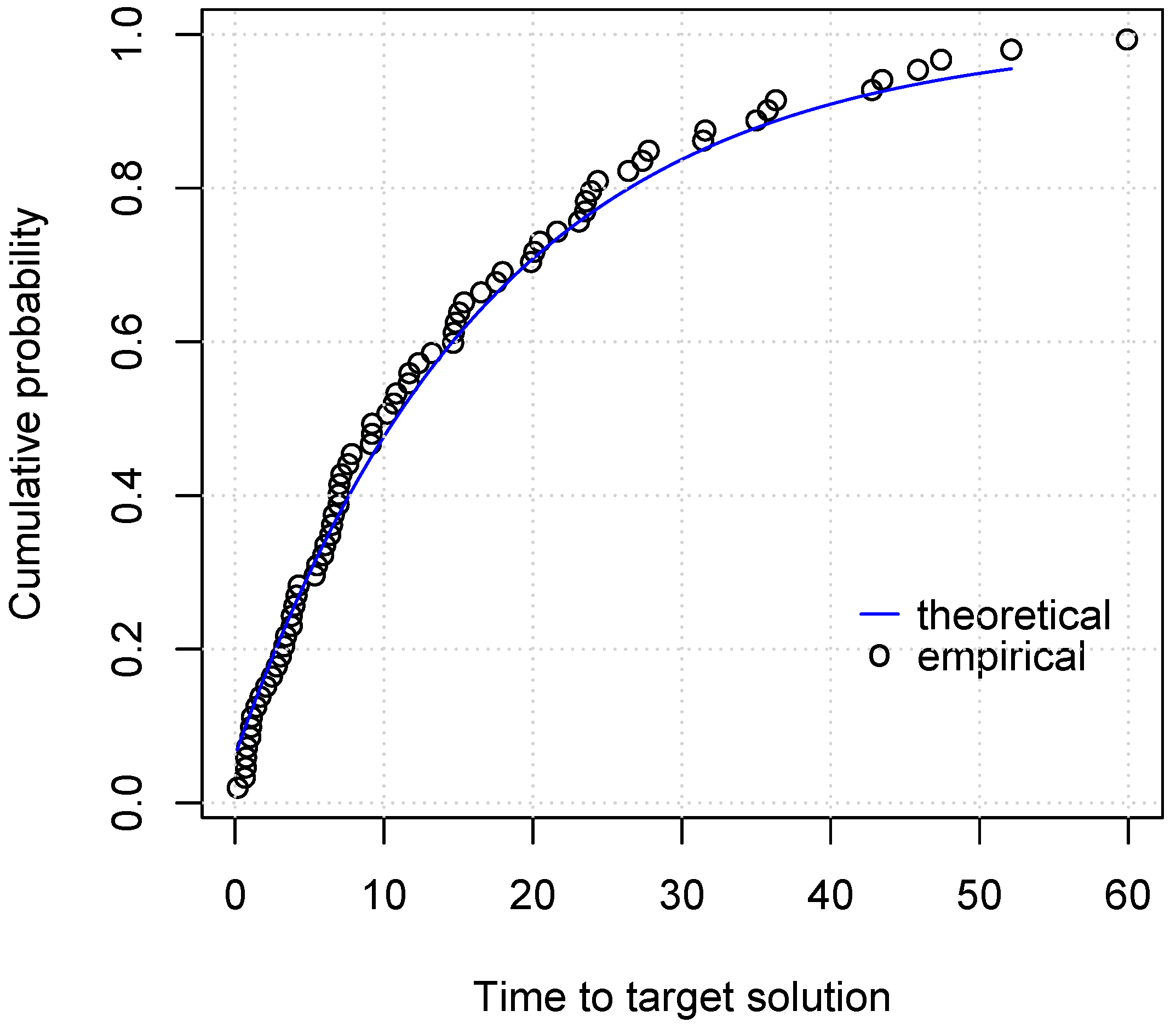
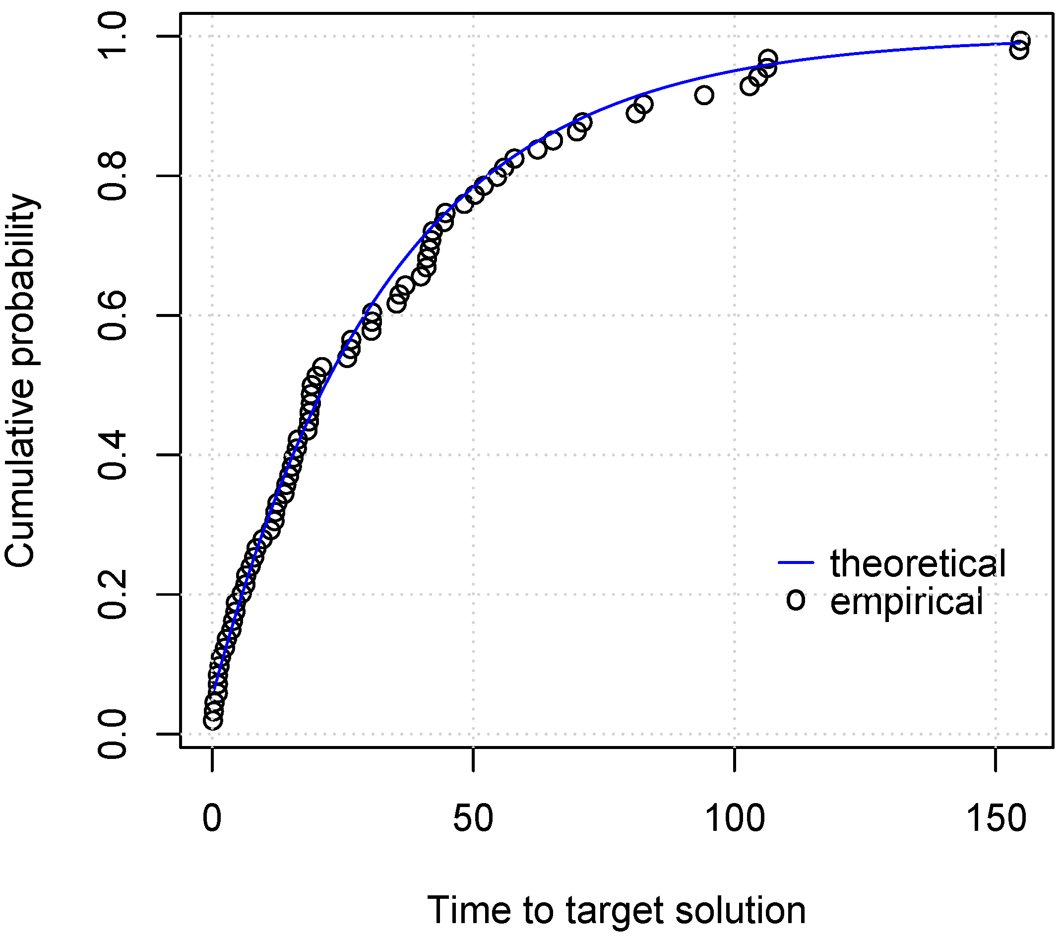
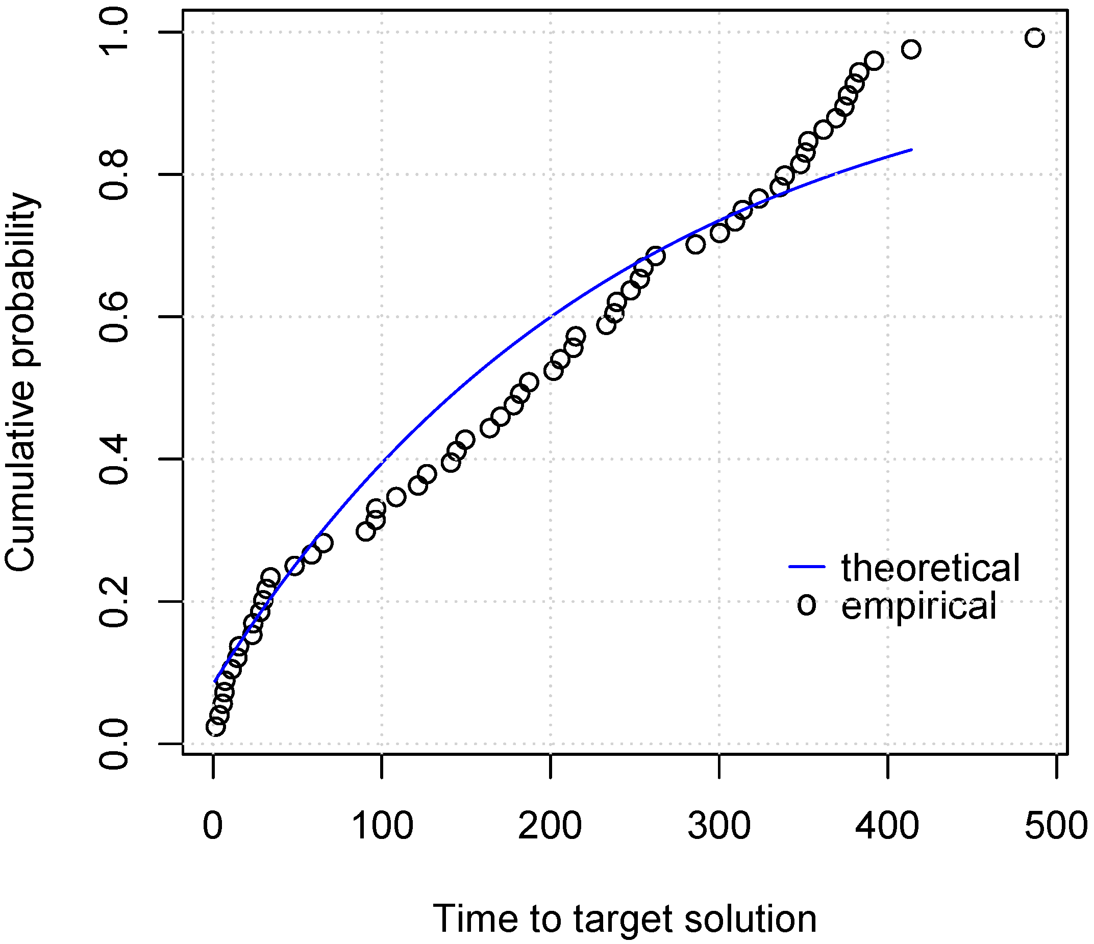
6.1. Synthetic Data Experiments

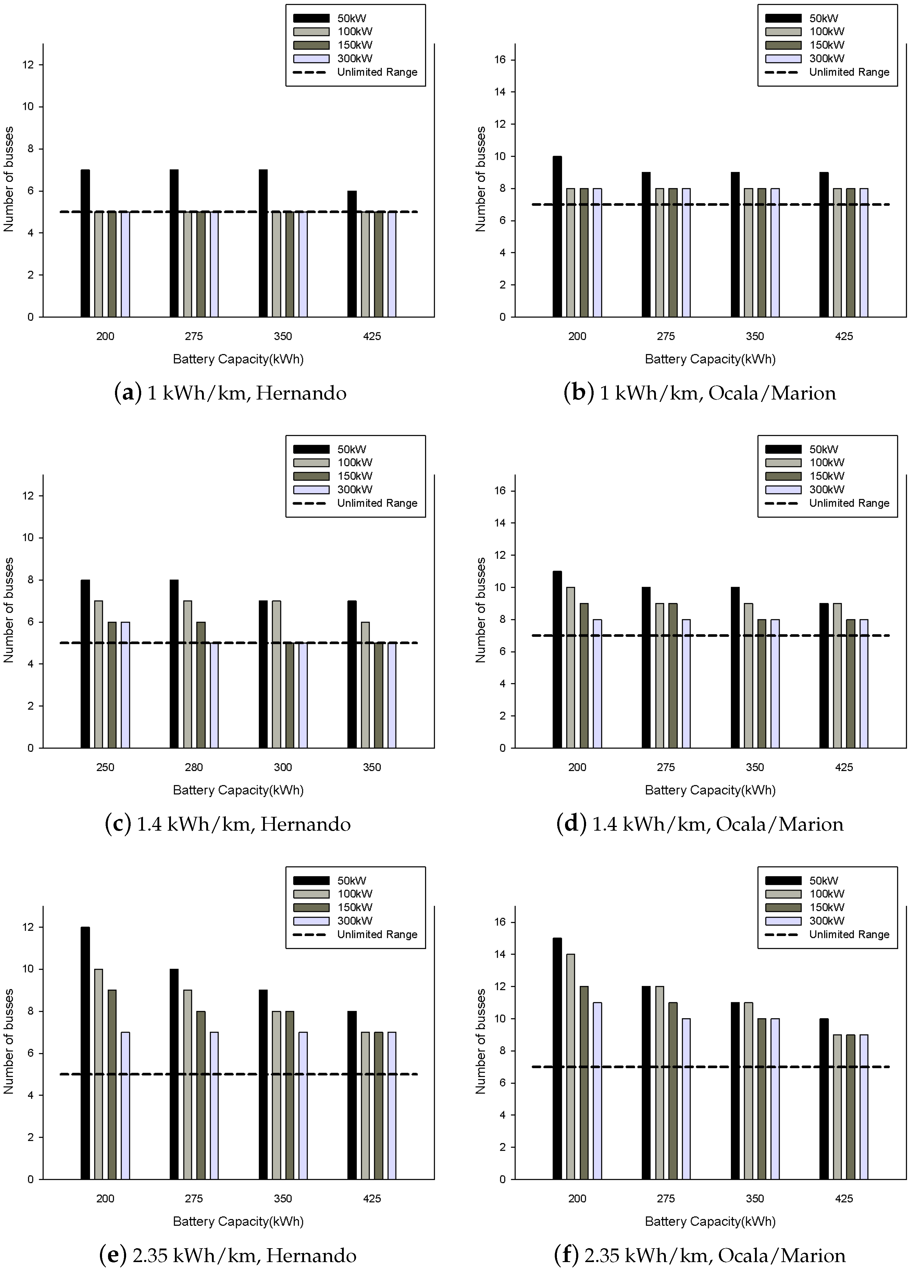
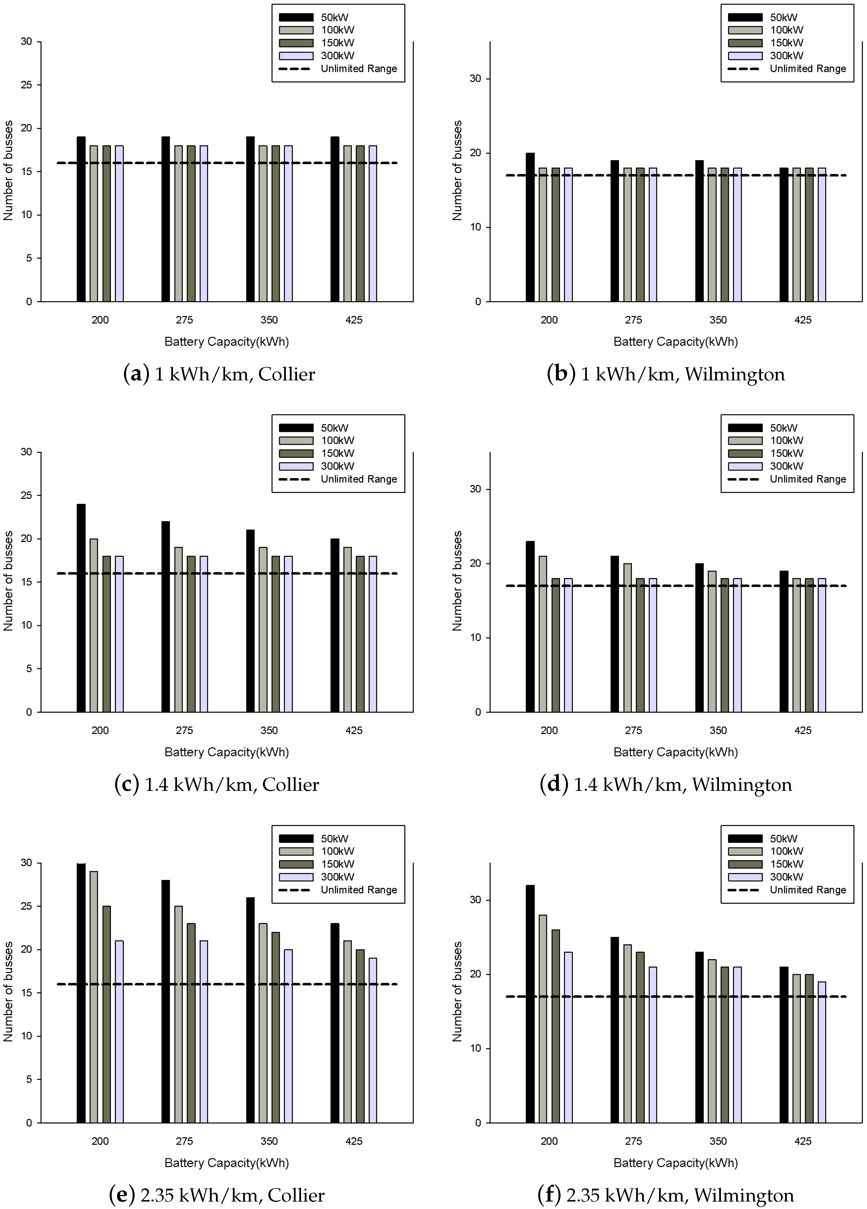
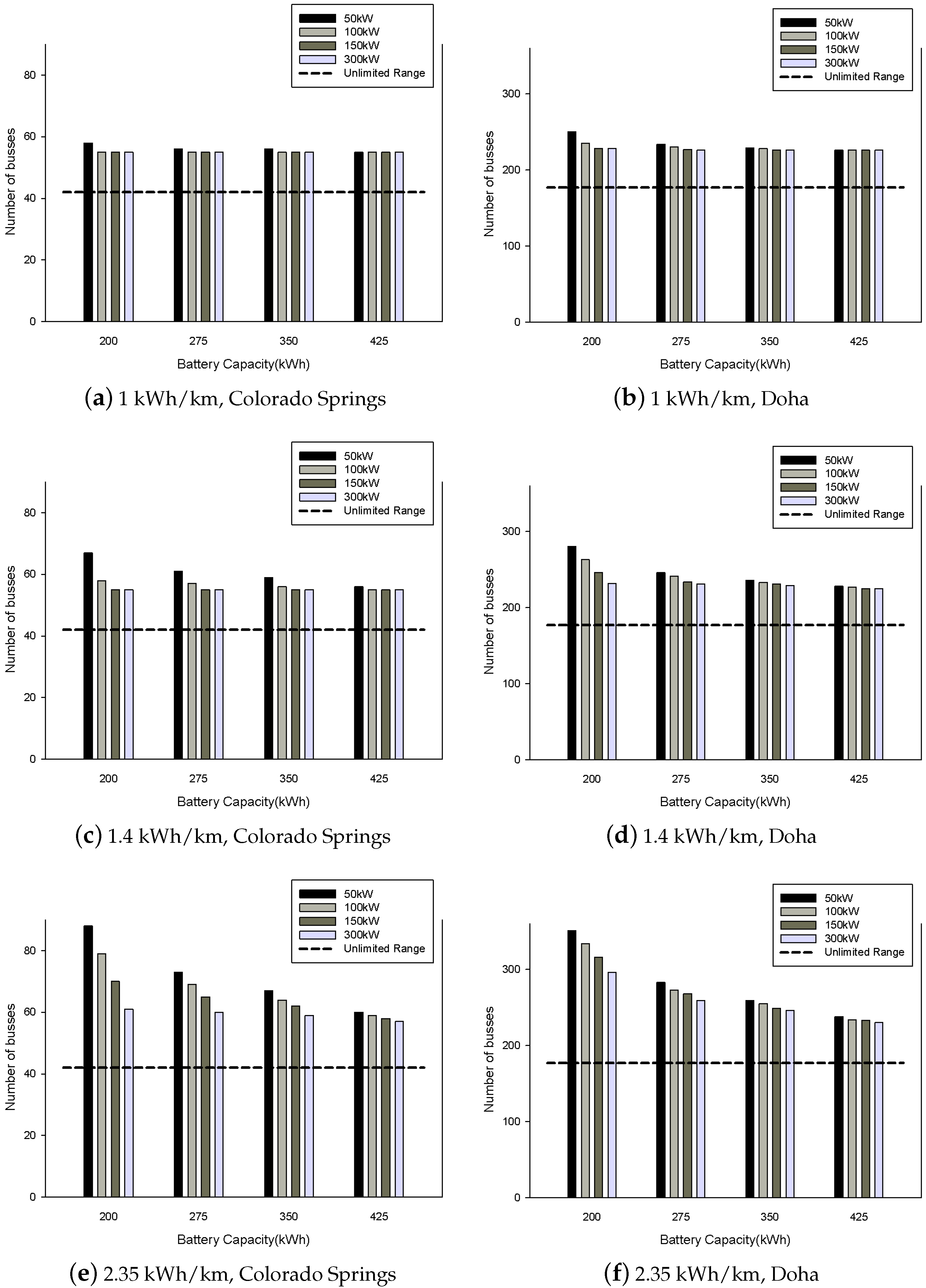
In this subsection, the experiments conducted on synthetic data are presented. A large number of problem instances is generated having a wide range of sizes. In this way, it is possible to have an extensive evaluation of the proposed GRASP and MIP approaches.

Let us start with providing details of the methods for generating such instances. The first step is randomly selecting N points in a square $(0,\alpha )\times (0,\alpha )$. Each point represents a location in the problem with one being selected as the depot. The distance between any two locations a and b is equal to the Euclidean distance between the corresponding points. The next stage is generating random bus routes. The scheduling is conducted over a time window of one day, and a period corresponds to one minute, or, equivalently, the problem is solved over 1440 periods. A bus route is defined by its origin $l_o$ and its destination $l_d$, the start time $t_s$ and the end time $t_e$, the duration d of a trip, and the frequency f of departure times. Note that the duration of a trip with some origin and destination locations is not directly related to the distance between them. The reason for this is that bus lines generally do not have a route that corresponds to the shortest path between the origin and the destination but instead try to satisfy the transport needs of passengers by visiting points of interest.

When generating the bus lines, the following rules have been used. A single location is randomly selected as the depot. Every other location $l\in L$ is an origin or destination of at least one bus line. The starting time, duration, and frequency of all bus lines are randomly selected from an interval $(s_{min},s_{max})$, $(d_{min},d_{max})$, and $(f_{min},f_{max})$, respectively. The ending time for each line is defined using its relation to the start time. To be more precise, it is equal to $t_s$ + $\delta$ where $\delta$ is randomly selected from $({\delta }_{min},{\delta }_{max})$. Individual trips for each line are generated in a natural way, having the form $(l_o,l_d,t_s+if,d)$ where an integer $i\ge 0$ is such that $t_s+if$ is less than the ending time.

To evaluate the MIP and the GRASP algorithms, the size of the problem instances has been related to the total number of trips R and varies from 20 to 2000. The number of locations depends on this value and is equal to $N=\sqrt{\frac{1}{2}R}$. An overview of the values of the parameters used for generating the synthetic problem instances can be seen in

Table 1. Parameters used to generate the synthetic problem instances.

Parameter	Min Value	Max Value
$\alpha$	50	50
T	1400	1400
s	300	420
d	30	60
$\delta$	720	900
f	60	120

.

The setting for the comparison of the MIP and the GRASP is as follows. The MIP has been solved in CPLEX with the default parameter setting with a time limit of 1200 s for each instance. In case of the GRASP, a total of 5000 iterations is performed, or, in other words, 5000 solutions are generated. The size of the RCL is 2. The aggregate results for each problem size are given in

Table 2. Comparison of the proposed GRASP and MIP for synthetic problem instances of different sizes.

Number of Trips	Average Solution			Found Optima		Average Time [s]
	GRASP	MIP	LB	GRASP	MIP	GRASP	MIP
20	3.60	3.60	3.60	10	10	0.42	0.79
30	5.10	4.80	4.80	7	10	0.75	159.01
40	6.00	6.20	5.00	3	3	1.15	884.53
50	7.20	7.70	5.61	0	0	1.54	1203.15
100	14.10	17.30	10.05	0	0	5.47	1206.40
200	26.60	39.30	18.50	0	0	20.48	1214.17
400	55.20	-	-	-	-	84.73	-
600	78.80	-	-	-	-	187.95	-
800	103.40	-	-	-	-	348.85	-
1000	130.10	-	-	-	-	571.24	-
1500	194.10	-	-	-	-	1479.20	-
2000	255.80	-	-	-	-	2855.66	-

. The averages of solutions and computational times are given. In addition, the average values of the lower bounds found by CPLEX and the number of found optimal solutions are also provided.

The first observation is that the MIP can find the proven optimal solutions for small problem instances having 20 to 40 trips, but not for all of them. The MIP could find feasible solutions and lower bounds for problem instances having up to 200 trips within the time limit of 1200 s. The GRASP algorithm managed to find 20 out of the 23 proven optimal solutions. In case of the problem sizes of 20 and 30 trips, for which the MIP found all the optimal solutions the average error of the GRASP is 0 and around 5%, respectively. The performance of the GRASP algorithm, evaluated by average solution quality, becomes better than the MIP starting from instances with 40 trips on. The difference between the average solution quality and the average lower bounds found by the MIP, in case of problem sizes where the MIP did not have a good performance, is significant and close to 50%. It is expected that the lower bounds provided by CPLEX are not tight.

The main reason for developing a metaheuristic for this problem is to provide a tool that can generate high quality feasible solutions for large problem instances within a reasonable time. The proposed GRASP algorithm achieves this by solving the instances with 2000 trips within less than an hour. In Table 2, the average computational times are included to provide insights to the scaling of the method. The computational time grows 100 times for instances of 100 and 200 trips to 1000 and 2000, respectively. This means that, in practice, the computational cost has a growth which is close to being quadratic.

With the goal of having a better understanding of the practical performance of the proposed method, in the sense of convergence speed, time-to-target plots (ttt-plots) are used to visualise runtime distributions. Such plots provide information about the probability that a method will find a solution at least as good as a given target value for a given problem instance within a given running time. This type of information is very useful for characterizing the running times of stochastic algorithms for combinatorial optimization problems. An extensive description of ttt-plots and tools for their generation can be found in [38,39].

The experimental setup for generating the ttt-plots is the following. Three different problems sizes having 400, 600, and 800 trips are evaluated. For each of them, one characteristic instance is selected and the proposed GRASP algorithm is run 75 times using different seeds for the random number generator. The number of generated solutions for each run is 10,000. A large number of generated solutions is used with the intention of having all the runs reach stagnation. The target value is the solution found with the minimal number of used eBuses. It should be noted that, in case of problem sizes 400 and 600, all the runs found the same quality solution. In case of the largest size, less than 5% of the runs did not find this solution and are excluded from generating the graph. The related ttt-plots can be seen in Figure 2, Figure 3 and Figure 4. From them, it can be observed that the computational cost for the GRASP algorithm, to find the solutions of the targeted quality, grows faster than quadratic. In case of instances having 400, 600, and 800 trips the time needed to have 80% of the runs find the solution of the desired quality is close to 25, 50, and 370 s. This is a common behavior for GRASP methods for large-scale problem instances, since it lacks a learning mechanism, and the relatively random search of the solution space is not very efficient for instances larger than some problem size.

In the final part of the analysis of the performance of the proposed GRASP algorithm, we make a comparison to other approaches for scheduling charging of eBuses. It should be noted that this is not a direct comparison, since the existing models focus on different properties of such system. In addition some of the methods find proven optimal solutions and others only near optimal ones. As previously stated, the goal of the proposed method is to find high quality solutions for large problem instances which correspond to real-world public transport systems. Because of this the comparison focuses on the size of instances such methods can solve as well as the computational cost.

In [29], a more complex model is proposed, which considers robust scheduling in a stochastic traffic environment. In this research, a branch-and-price algorithm is used to find approximate solutions to problem instances of at most 96 trips with a computational cost of 117 s. In the work by Awesabi et al. [28], a wireless setting of single-depot dynamic charging systems is considered and the system is optimized using a MIP approach. This model also considers the optimization of the battery size of the used eBuses. The proposed method optimizes a small off-campus college transportation system having six routes. A cost optimization of a public transport system based on eBuses is provided in [30]. In this work the proposed MIP is solved using a combination of column generation and Lagrangian relaxation for a system having four routes and 543 trips with a computational cost of 539 s. To the best of the authors knowledge, the largest problem instances for eBus scheduling have been solved using a column generation-based approach combined with a local search [36]. In this work, problem instances having 941 trips are solved within a time period of 46 to 58 hours. It can be observed that the proposed GRASP algorithm manages to solve much larger instances at a significantly lower computational cost. To be more precise, the conducted computational experiments indicate that an average of less than 3000 s is needed to find high quality solutions for instances having 2000 trips. This increased computational efficiency makes it possible to conduct an extensive analysis of real-world systems as it will be seen in the following case studies.

6.2. Case Studies

In this section, the results of case studies on real-world public transport systems are presented. The computational experiments are conducted using the previously presented GRASP algorithm. The procedure for generating test instances for the selected public transport systems is as follows. The used timetables for each case study are obtained from official sources available online. The used data for bus lines include the origin and destination locations and the departure and arrival times for each of the trips performed by a bus. The departure and arrival times are mapped to time periods in the model in which a single time period had the length of one minute. Note that, some bus lines are circular and some are bi-directional. In case of bi-directional lines, a trip would correspond to one direction of travel. The distance between locations is calculated based on Googlemaps using the Google Cloud Services. Traffic conditions have not been considered in the model.

The tests are used to evaluate the effect of different battery capacities and charging powers on the number of EBs needed to achieve a public transport timetable. The battery capacity of EBs commonly used for this task is from 200 kWh to 425 kWh [40]. The charging power used for EBs can greatly vary based on the installed selected infrastructure [41]. In the conducted computational experiments, a charging range between 50 kW and 300 kW is considered. Contrary to DBs, the range of EBs has a much larger level of variety [42,43] which especially depends on driver habits and weather conditions. Empirical studies have shown that the consumption for 12 foot EBs averages around 1.4 kWh/km, but can range from 1 kWh/km in case of an experienced driver in ideal conditions to even 2.35 kWh/km in extremely cold weather when electric heating is used [44]. In the conducted case studies the average energy consumption and the two extreme values are evaluated. In the case studies, the speed of EBs is considered constant and equal to 20 km/h [45,46]. The cities/counties chosen for the case studies have been selected in a way to represent public transport systems having a wide range of different properties. In the following text the relevant details are provided.

The Ocala/Marion County, Florida, USA system consists of seven bus lines. Most of the lines are bi-directional and have departures every hour in each direction. The trip in each direction has a duration of around 20–30 min. All the bus lines start their trips from a central terminal. As a second case study, the Hernando, Florida, USA system with only four bidirectional lines is chosen. The line’s length and departure frequencies are similar to the case of Ocala/Marion County. The system does not have a main terminal; instead, the lines connect different locations in the city.

The third case study is the Collier, Florida, USA system with 20 lines, half of which are circular bus lines. This bus network has one main terminal and around half of the lines use this terminal as an arrival or departure station. The frequencies vary from 60 to 160 min, with the majority of lines having departures every 90 min. The duration of lines ranges from 35–80 min, with the majority being 40 min. The fourth case study, the Wilmington, North Carolina, USA system has close to 20 circular lines. The vast majority of the lines have an hourly frequency and a duration of close to an hour. The system has two main terminals from which most of the buses depart.

The fifth case is the Colorado Springs, Colorado, USA system which has around 30, mostly bi-directional, bus lines. The majority of bus lines have frequencies of 15, 30, and 60 min. The duration of most of the trips would be 20–30 min. The system has four main stations and the majority of the lines have a departure station at one of them. As a sixth case study, the Doha, Qatar system with 50 bus lines is considered. Nearly half of the bus lines are circular. The majority of the lines have 20 and 30 minute frequencies. There are also two large terminals from which most of the buses depart. In addition there is a group of lines that depart from the airport. One characteristic of the Doha system is that the lines have a long duration ranging from 60 to even 180 min.

The locations of the bus depots for all the tested cities are not available. On the other hand, currently all these transport systems are operated using DBs so there is a potential for changing the location of the EB depot due to power distribution requirements for the installation of chargers. In the generated test instances, the locations of the depots are selected by choosing empty locations that are close to the largest terminal in the system.

It should be noted that, in case of Doha and the other systems having major terminals, the arrival times and departure times are set in a way to maximize the possibility of passengers changing lines. This results in the corresponding problem instances becoming much harder to solve by the MIP compared to the synthetic ones. This is due to an increased level of symmetries in the solutions space, which does not notably effect the GRASP algorithm.

The objective of the conducted case studies is to evaluate the number of EBs needed to cover a public transport timetable. This is done through a comparison of the number of DBs needed to achieve the same task. DBs, in general, have ranges that are sufficient to perform all the daily trips on a full tank. In practice this means that in this case the range constraints are not relevant. Consequently, the number of DBs needed to achieve a timetable can be acquired using a MIP having the objective function given in Equation (6) and only the constraints in (9)–(11). This model is significantly less computationally expensive than the one for EBs. These simplified problem instances generated for the systems used in the case studies can all be solved to optimality using CPLEX within less than 10 min.

Before presenting results of the conducted computational experiments, let us point out the following. The GRASP algorithm finds high quality solutions for EB-based systems which are compared to the optimal ones found by the MIP for DBs. Consequently, the provided results are used to analyze trends and not to provide exact configurations of the systems. In case of using the proposed GRASP algorithm to practical real-world systems, with the intention of optimizing them, the method has a significant drawback of not being able to evaluate the precise distance from an optimal solution. Because of this, for such applications, it would be essential to conduct a more in-depth error analysis through finding tight lower bounds. It should be noted that this is a simplification of the real-world problem that does not consider driver-related constraints. Such constraints in many cases also impact the number of buses needed to perform all the trips in a public transport timetable.

The summary of the results is presented in Figure 5, Figure 6 and Figure 7 for different system sizes. For each city, a subfigure is used to show the number of EBs needed to perform a timetable for different combinations of EB battery capacities, charging powers at the depot, and energy consumption per unit distance. The first thing that can be observed is that, in case of ideal conditions with 1 kWh/km energy consumption, the increase in the needed EBs compared to DBs, is generally relatively small for small and medium systems. In case of large systems, the increase is more significant and can reach even 30%. It should be noted, that GRASP algorithms generally have a worse performance for large problem instances and it is expected that part of the increase is related to this fact. In case of all tested systems, it is noticeable that the use of higher charging powers has a more significant impact than the battery capacities. An increase in charging power at the depot decreases the time needed to charge an EB. The impact of increasing charging power is the most significant for low battery capacity EBs, but is significant for all of them.

The difference in the number of EBs needed in case of average energy consumption compared to the extreme case is very significant. Once more this increase is most notable in case of low charging powers and battery capacities. It should be understood that although the extreme energy consumption events are rare, it is expected that they will occur annually during periods of extreme weather. The results indicate that it can be extremely beneficial adding alternative energy sources for heating and cooling. Another observation that can be made is that, in case of larger initial investments, longer range EBs, and higher power chargers, the fluctuation in the number of needed EBs during the year can be greatly reduced.

7. Conclusions

In this paper, the practical problem of using electric buses in public transport systems has been analyzed. The addressed problem consists of scheduling EBs to perform all the trips in a public transport timetable. This has been done by firstly developing a mathematical model for a single-depot system in which EB charging times depend on the current state of the battery. Due to the fact that the developed MIP model can only solve small-scale problem instances, that do not reflect real-world systems, a metaheuristic approach has also been developed. To be more precise, a GRASP algorithm has been created that can solve problem instances that correspond to urban public transport systems. The effectiveness of the GRASP algorithm has been evaluated through a comparison with optimal solutions acquired using the MIP for small instances. The conducted computational experiments have shown that the GRASP manages to find many optimal or near optimal solutions for those instances. The computational cost of the GRASP algorithm is significantly lower than of the MIP. It manages to find better solutions than the MIP, even for relatively small instances, where the MIP terminates early and can find solutions for problem sizes on which the MIP cannot be applied.

The developed GRASP algorithm has been used for case studies on real-world public transport systems. The related computational experiments have shown that the number of EBs needed to achieve a public transport timetable can be significantly higher than DBs. The developed model indicates that by using high speed chargers the number of needed EBs can be greatly reduced and using this type of chargers is more relevant than the range of the EBs. In addition, systems using higher charging powers and having EB fleets with larger battery capacities have a much lower seasonal fluctuation in the number of needed EBs. The results of the conducted case studies provide valuable insights for the cost analysis of such systems.

In the future there are several directions in which the presented research can be extended. The first one is extending the model to include multiple-charging depots, limiting the charging capacities, considering driver-related constraints and different types of disturbances in a stochastic model. It should be noted that the used solution method, the GRASP, is very suitable for parallelization. This type of speedup would be highly relevant for such extended models. Another direction is adapting the proposed GRASP algorithm to previously developed mathematical models related to the use of EBs. This can enable the application of such model to much larger problem instances that well represent real-world systems. Another issue relates to disturbances in public transport (see [47] for a survey and [48] for some conceptional work) as they can even arise with special features related to EBs (see, e.g., [49]). Finally, the Fixed Set Search metaheuristic [50], which adds a learning mechanism to GRASP, can be applied to try to increase the quality of found solutions for the problem of interest.

References

1. Batur, İ.; Bayram, I.S.; Koc, M. Impact assessment of supply-side and demand-side policies on energy consumption and CO2 emissions from urban passenger transportation: The case of Istanbul. J. Clean. Prod. 2019, 219, 391–410. [Google Scholar] [CrossRef] [Green Version]
2. Meyer, D.; Wang, J. Integrating ultra-fast charging stations within the power grids of smart cities: A review. IET Smart Grid 2018, 1, 3–10. [Google Scholar] [CrossRef]
3. Rahman, I.; Vasant, P.M.; Singh, B.S.M.; Abdullah-Al-Wadud, M.; Adnan, N. Review of recent trends in optimization techniques for plug-in hybrid, and electric vehicle charging infrastructures. Renew. Sustain. Energy Rev. 2016, 58, 1039–1047. [Google Scholar] [CrossRef]
4. Jovanovic, R.; Bayhan, S.; Bayram, I.S. A multiobjective analysis of the potential of scheduling electrical vehicle charging for flattening the duck curve. J. Comput Sci. 2021, 48, 101262. [Google Scholar] [CrossRef]
5. Song, Z.; Liu, Y.; Gao, H.; Li, S. The underlying reasons behind the development of public electric buses in China: The Beijing case. Sustainability 2020, 12, 688. [Google Scholar] [CrossRef] [Green Version]
6. Malnaca, K.; Gorobetz, M.; Yatskiv (Jackiva), I.; Korneyev, A. Decision-making process for choosing technology of diesel bus conversion into electric bus. In Reliability and Statistics in Transportation and Communication; Kabashkin, I., Yatskiv (Jackiva), I., Prentkovskis, O., Eds.; Springer International Publishing: Cham, Switzerland, 2019; pp. 91–102. [Google Scholar]
7. Topal, O.; Nakir, İ. Total cost of ownership based economic analysis of diesel, CNG and electric bus concepts for the public transport in Istanbul City. Energies 2018, 11, 2369. [Google Scholar] [CrossRef] [Green Version]
8. Quarles, N.; Kockelman, K.M.; Mohamed, M. Costs and benefits of electrifying and automating bus transit fleets. Sustainability 2020, 12, 3977. [Google Scholar] [CrossRef]
9. Feng, W.; Figliozzi, M. Vehicle technologies and bus fleet replacement optimization: Problem properties and sensitivity analysis utilizing real-world data. Public Transp. 2014, 6, 137–157. [Google Scholar] [CrossRef]
10. Zahedmanesh, A.; Muttaqi, K.M.; Sutanto, D. A cooperative energy management in a virtual energy hub of an electric transportation system powered by PV generation and energy storage. IEEE Trans. Transp. Electrif. 2021, 7, 1123–1133. [Google Scholar] [CrossRef]
11. Vuelvas, J.; Ruiz, F.; Gruosso, G. Energy price forecasting for optimal managing of electric vehicle fleet. IET Electr. Syst. Transp. 2020, 10, 401–408. [Google Scholar] [CrossRef]
12. Gallo, J.B.; Bloch-Rubin, T.; Tomić, J. Peak Demand Charges and Electric Transit Buses; U.S. Department of Transportation Federal Transit Administration: Washington, DC, USA, 2014. [Google Scholar]
13. Dreier, D.; Rudin, B.; Howells, M. Comparison of management strategies for the charging schedule and all-electric operation of a plug-in hybrid-electric bi-articulated bus fleet. Public Transp. 2020, 12, 363–404. [Google Scholar] [CrossRef]
14. Foster, B.A.; Ryan, D.M. An integer programming approach to the vehicle scheduling problem. J. Oper. Res. Soc. 1976, 27, 367–384. [Google Scholar] [CrossRef]
15. Desaulniers, G.; Hickman, M.D. Public transit. Handb. Oper. Res. Manag. Sci. 2007, 14, 69–127. [Google Scholar] [CrossRef]
16. Wen, M.; Linde, E.; Ropke, S.; Mirchandani, P.; Larsen, A. An adaptive large neighborhood search heuristic for the electric vehicle scheduling problem. Comput. Oper. Res. 2016, 76, 73–83. [Google Scholar] [CrossRef] [Green Version]
17. Freling, R.; Paixão, J.M.P. Vehicle scheduling with time constraint. In Computer-Aided Transit Scheduling; Daduna, J.R., Branco, I., Paixão, J.M.P., Eds.; Springer: Berlin/Heidelberg, Germany, 1995; pp. 130–144. [Google Scholar] [CrossRef]
18. Haghani, A.; Banihashemi, M. Heuristic approaches for solving large-scale bus transit vehicle scheduling problem with route time constraints. Transp. Res. Part A Policy Pract. 2002, 36, 309–333. [Google Scholar] [CrossRef]
19. Desaulniers, G.; Desrosiers, J.; Solomon, M.M.; Soumis, F.; Villeneuve, D. A unified framework for deterministic time constrained vehicle routing and crew scheduling problems. In Fleet Management and Logistics; Springer: Berlin/Heidelberg, Germany, 1998; pp. 57–93. [Google Scholar]
20. Perumal, S.S.; Dollevoet, T.; Huisman, D.; Lusby, R.M.; Larsen, J.; Riis, M. Solution approaches for integrated vehicle and crew scheduling with electric buses. Comput. Oper. Res. 2021, 132, 105268. [Google Scholar] [CrossRef]
21. Iliopoulou, C.; Kepaptsoglou, K.; Vlahogianni, E. Metaheuristics for the transit route network design problem: A review and comparative analysis. Public Transp. 2019, 11, 487–521. [Google Scholar] [CrossRef]
22. Durán-Micco, J.; Vansteenwegen, P. A survey on the transit network design and frequency setting problem. Public Transp. 2021. [Google Scholar] [CrossRef]
23. Liu, Z.; Song, Z. Robust planning of dynamic wireless charging infrastructure for battery electric buses. Transp. Res. Part C Emerg. Technol. 2017, 83, 77–103. [Google Scholar] [CrossRef]
24. Xylia, M.; Leduc, S.; Patrizio, P.; Kraxner, F.; Silveira, S. Locating charging infrastructure for electric buses in Stockholm. Transp. Res. Part C Emerg. Technol. 2017, 78, 183–200. [Google Scholar] [CrossRef]
25. Wang, J.; Kang, L.; Liu, Y. Optimal scheduling for electric bus fleets based on dynamic programming approach by considering battery capacity fade. Renew. Sustain. Energy Rev. 2020, 130, 109978. [Google Scholar] [CrossRef]
26. Ji, J.; Bie, Y.; Shen, B. Vehicle scheduling model for an electric bus line. In Smart Transportation Systems 2020; Springer: Berlin/Heidelberg, Germany, 2020; pp. 29–39. [Google Scholar]
27. Liu, T.; Ceder, A.A. Battery-electric transit vehicle scheduling with optimal number of stationary chargers. Transp. Res. Part C Emerg. Technol. 2020, 114, 118–139. [Google Scholar] [CrossRef]
28. Alwesabi, Y.; Wang, Y.; Avalos, R.; Liu, Z. Electric bus scheduling under single depot dynamic wireless charging infrastructure planning. Energy 2020, 213, 118855. [Google Scholar] [CrossRef]
29. Tang, X.; Lin, X.; He, F. Robust scheduling strategies of electric buses under stochastic traffic conditions. Transp. Res. Part C Emerg. Technol. 2019, 105, 163–182. [Google Scholar] [CrossRef]
30. Van Kooten Niekerk, M.E.; van den Akker, J.; Hoogeveen, J. Scheduling electric vehicles. Public Transp. 2017, 9, 155–176. [Google Scholar] [CrossRef]
31. Janovec, M.; Koháni, M. Exact approach to the electric bus fleet scheduling. Transp. Res. Proc. 2019, 40, 1380–1387. [Google Scholar] [CrossRef]
32. Zhou, G.; Xie, D.; Zhao, X.; Lu, C. Collaborative optimization of vehicle and charging scheduling for a bus fleet mixed with electric and traditional buses. IEEE Access 2020, 8, 8056–8072. [Google Scholar] [CrossRef]
33. Yao, E.; Liu, T.; Lu, T.; Yang, Y. Optimization of electric vehicle scheduling with multiple vehicle types in public transport. Sustain. Cities Soc. 2020, 52, 101862. [Google Scholar] [CrossRef]
34. Li, L.; Lo, H.K.; Xiao, F. Mixed bus fleet scheduling under range and refueling constraints. Transp. Res. Part C Emerg. Technol. 2019, 104, 443–462. [Google Scholar] [CrossRef]
35. Feo, T.A.; Resende, M.G. Greedy randomized adaptive search procedures. J. Global Optim. 1995, 6, 109–133. [Google Scholar] [CrossRef] [Green Version]
36. Li, J.Q. Transit bus scheduling with limited energy. Transp. Sci. 2014, 48, 521–539. [Google Scholar] [CrossRef]
37. Stakić, Đ.; Anokić, A.; Jovanovic, R. Comparison of different grasp algorithms for the heterogeneous vector bin packing problem. In Proceedings of the 2019 China-Qatar International Workshop on Artificial Intelligence and Applications to Intelligent Manufacturing (AIAIM), Doha, Qatar, 1–4 January 2019; pp. 63–70. [Google Scholar] [CrossRef]
38. Aiex, R.M.; Resende, M.G.; Ribeiro, C.C. TTT plots: A perl program to create time-to-target plots. Optim. Lett. 2007, 1, 355–366. [Google Scholar] [CrossRef]
39. Reyes, A.; Ribeiro, C.C. Extending time-to-target plots to multiple instances. Int. Trans. Oper. Res. 2018, 25, 1515–1536. [Google Scholar] [CrossRef]
40. Gao, Z.; Lin, Z.; LaClair, T.J.; Liu, C.; Li, J.M.; Birky, A.K.; Ward, J. Battery capacity and recharging needs for electric buses in city transit service. Energy 2017, 122, 588–600. [Google Scholar] [CrossRef] [Green Version]
41. Conti, V.; Orchi, S.; Valentini, M.P.; Nigro, M.; Calò, R. Design and evaluation of electric solutions for public transport. Transp. Res. Procedia 2017, 27, 117–124. [Google Scholar] [CrossRef]
42. Vepsäläinen, J.; Ritari, A.; Lajunen, A.; Kivekäs, K.; Tammi, K. Energy uncertainty analysis of electric buses. Energies 2018, 11, 3267. [Google Scholar] [CrossRef] [Green Version]
43. Pamuła, T.; Pamuła, W. Estimation of the energy consumption of battery electric buses for public transport networks using real-world data and deep learning. Energies 2020, 13, 2340. [Google Scholar] [CrossRef]
44. SustainableBus. Electric Bus Range, Focus on Electricity Consumption. A Sum-Up. 2021. Available online: https://www.sustainable-bus.com/news/electric-bus-range-focus-on-electricity-consumption-a-sum-up/ (accessed on 9 September 2021).
45. Chao, Z.; Xiaohong, C. Optimizing battery electric bus transit vehicle scheduling with battery exchanging: Model and case study. Procedia-Soc. Behav. Sci. 2013, 96, 2725–2736. [Google Scholar] [CrossRef] [Green Version]
46. Mahesh, S.; Ramadurai, G. Analysis of driving characteristics and estimation of pollutant emissions from intra-city buses. Transp. Res. Procedia 2017, 27, 1211–1218. [Google Scholar] [CrossRef]
47. Ge, L.; Voß, S.; Xie, L. Robustness and Disturbances in Public Transport; Technical Report; Institute of Information Systems, Leuphana University of Lüneburg and Institute of Information Systems (IWI), University of Hamburg: Hamburg, Germany, 2020. [Google Scholar]
48. Dekker, M.M.; van Lieshout, R.N.; Ball, R.C.; Bouman, P.C.; Dekker, S.C.; Dijkstra, H.A.; Goverde, R.M.P.; Huisman, D.; Panja, D.; Schaafsma, A.A.M.; et al. A next step in disruption management: Combining operations research and complexity science. Public Transp. 2021. [Google Scholar] [CrossRef]
49. Vepsäläinen, J.; Kivekäs, K.; Otto, K.; Lajunen, A.; Tammi, K. Development and validation of energy demand uncertainty model for electric city buses. Transp. Res. D Transp. Environ. 2018, 63, 347–361. [Google Scholar] [CrossRef]
50. Jovanovic, R.; Voss, S. The fixed set search applied to the power dominating set problem. Expert Syst. 2020, 37, e12559. [Google Scholar] [CrossRef]
Figure 1. Illustration of the conversion of a timetable with known distances between origins and destinations between trips. The directed graph (middle) has a node for each trip and edges only connect trips that can be sequentially done. The set of red edges (bottom) is a schedule of EBs. It contains the two buses with schedules ( D e p o t , a , c , D e p o t ) and ( D e p o t , b , d , D e p o t ) .
Energies 14 06610 g001aEnergies 14 06610 g001b
Figure 2. Time-to-target plot for an instance with 400 trips based on 75 independent runs of the GRASP algorithm.
Energies 14 06610 g002
Figure 3. Time-to-target plot for an instance with 600 trips based on 75 independent runs of the GRASP algorithm.
Energies 14 06610 g003
Figure 4. Time-to-target plot for an instance with 800 trips based on 75 independent runs of the GRASP algorithm.
Energies 14 06610 g004
Figure 5. Number of EBs with different ranges dependent on depot charging power to achieve a small public bus transport system. In each of the subfigures the dashed line corresponds to the number of DBs needed for the same task.
Energies 14 06610 g005
Figure 6. Number of EBs with different ranges dependent on depot charging power to achieve a medium public bus transport system. In each of the subfigures the dashed line corresponds to the number of DBs needed for the same task.
Energies 14 06610 g006
Figure 7. Number of EBs with different ranges dependent on depot charging power to achieve a large public bus transport system. In each of the subfigures the dashed line corresponds to the number of DBs needed for the same task.
Energies 14 06610 g007