Dynamic Blackout Probability Monitoring System for Cruise Ship Power Plants

Abstract

Stringent environmental regulations and efforts to improve the shipping operations sustainability have resulted in designing and employing more complex configurations for the ship power plants systems and the implementation of digitalised functionalities. Due to these systems complexity, critical situations arising from the components and subsystem failures, which may lead to accidents, require timely detection and mitigation. This study aims at enhancing the safety of ship complex systems and their operation by developing the concept of an integrated monitoring safety system that employs existing safety models and data fusion from shipboard sensors. Detailed Fault Trees that model the blackout top event, representing the sailing modes of a cruise ship and the operating modes of its plant, are employed. Shipboard sensors’ measurements acquired by the cruise ship alarm and monitoring system are integrated with these Fault Trees to account for the acquired shipboard information on the investigated power plant configuration and its components operating conditions, thus, facilitating the estimation of the blackout probability time variation as well as the dynamic criticality assessment of the power plant components. The proposed concept is verified by using a virtual simulation environment developed in Matlab/Simulink. This study supports the dynamic assessment of the ship power plants and therefore benefits the decision-making for enhancing the plant safety during operations.

1. Introduction

The maritime industry pillars the world trade as it transports around 90% of goods in volume and 70% in value [1]. Apart from cargo transfer, the cruise ship industry has exhibited substantial growth the last decade [2]. To support the functions and improve the sustainability of modern cruise industry, highly sophisticated cruise ships have been designed and built, which employ advanced propulsion and power plant systems, compartment arrangement and exterior design. It is widely acknowledged that the modern cruise ships are the most technologically sophisticated ships compared to other ship types.

The cruise ship industry is a highly competitive market that has been rapidly developing with both the vessels’ size and number constantly increasing [2]. As cruise ships carry large numbers of passengers and crew, it is paramount to ensure the safety considering humans, assets, environment and business. Potential power system malfunctions, such as blackout may lead to collision, contact or grounding, which, in turn, may end up in significant human losses as well as severe environmental pollution [3,4]. This may also severely damage the financial and social profile of the cruise ship operator, and respectively of the whole cruise industry. The recent total blackout incident on-board of the Viking Sky [5], where all the generator sets in both engine rooms shut down, provides a representative example of the potential safety, financial and social implications associated with blackout events. In this respect, it is important to minimise the blackout probability of the cruise ships’ power plants design as well as to ascertain that adequate power will be available when required [6].

Another critical parameter is the significant cognitive load imposed by the ship systems on the cruise ships’ crews and operators with respect to prevention of accidents and incidences [7]. The cruise ships power and propulsion systems are categorized as complex cyber-physical systems [8] consisting of a significant number of heterogeneous components, interacting with each other in multiple ways. Such complexity leads to significant number of alarms that the crew must deal with constantly [9], whilst it may hinder the classification of the critical alarms. This type of cognitive operator overload has been identified as one of the contributory factors to the Three Mile Island nuclear reactor accident [8,10]. In the recent blackout case on a cruise ship, the crew accepted and cleared low lubrication oil alarms (the reason for this were not reported), which in combination with heavy roll and pitch led to loss of three Diesel Generators (DGs) out of the four of this ship power plant [11].

One potential solution to overcome the problem of cognitive load is to combine sensors and alarms with system safety models, rather than to use them independently from each other in specifically dedicated devices. The role of such automated safety monitoring devices “is to detect conditions that signal potentially hazardous disturbances and assist the operators of the system in the timely control of those disturbances” [12]. The idea of using sensor measurements for safety enhancement during operations was introduced during the 1980s decade. For example, Ref. [12] used those elements in condition monitoring systems.

Numerous studies focused on integrating safety models with sensor measurements on other systems. Hu et al. [13] used a Bayesian network model for integrating condition monitoring and inspection data for risk assessment of a nuclear power plant system allowing for a more effective system health estimation compared with approaches based on the traditional Event Trees. Jinqiu et al. [14] used Hazard and Operability study results to develop a dynamic Bayesian network for a gas turbine compressor system integrating sensor measurements. In a follow-up study [15], the previously developed dynamic Bayesian network was applied to the gas turbine compressor for the purposes of risk assessment. Aizpurua et al. [16,17] integrated the prognostics estimations for power distribution system with Boolean Driven Markov Processes and Stochastic Activity networks. Gomes et al. [18] combined Fault Trees with prognostics based remaining useful life estimation for an aircraft system. Pattison et al. [19] have integrated the dynamic Bayesian networks with random forests and memetic algorithms for the development of real-time maintenance system for windfarms.

Nonetheless, very few studies focused on the ship propulsion systems. Abaei et al. [20] have employed multinominal process trees and hierarchical Bayesian inference for predicting failures in machinery systems in the context of unmanned vessels. Eriksen et al. [21] applied a modified version of Failure Modes and Effects Analysis for more effective maintenance of unmanned ship systems. However, both studies did not consider the utilisation of the sensor measurements for dynamic risk analysis.

This study aims at the development and demonstration of a potential blackout monitoring system for a cruise ship power plant system integrated with sensor measurements. The novelty of this study stems from: (a) an application and an advancement of the concept of integrating sensor measurements with safety methods to monitor and prevent blackout event in cruise ships power plants; (b) development of a methodology for concept demonstration in a virtual simulation environment, and; (c) verification of the concept in this virtual environment. Whilst this study employs material from previous publications on cruise ship power plants, it improves the current state-of-the-art knowledge by demonstrating how the existing safety methods can be fused with sensors measurements and integrated with reliability data to develop a safety monitoring system that predicts the selected safety metrics time variations.

The remaining of this study is structured as follows. Section 2 elaborates the proposed methodology for concept development and verification. In Section 3, the information about the investigated system is provided. Section 4 presents and discusses the derived simulation results as well as provides recommendations for further developing the proposed safety system. Section 5 summarises the min findings and the conclusions of this study.

2. Materials and Methods

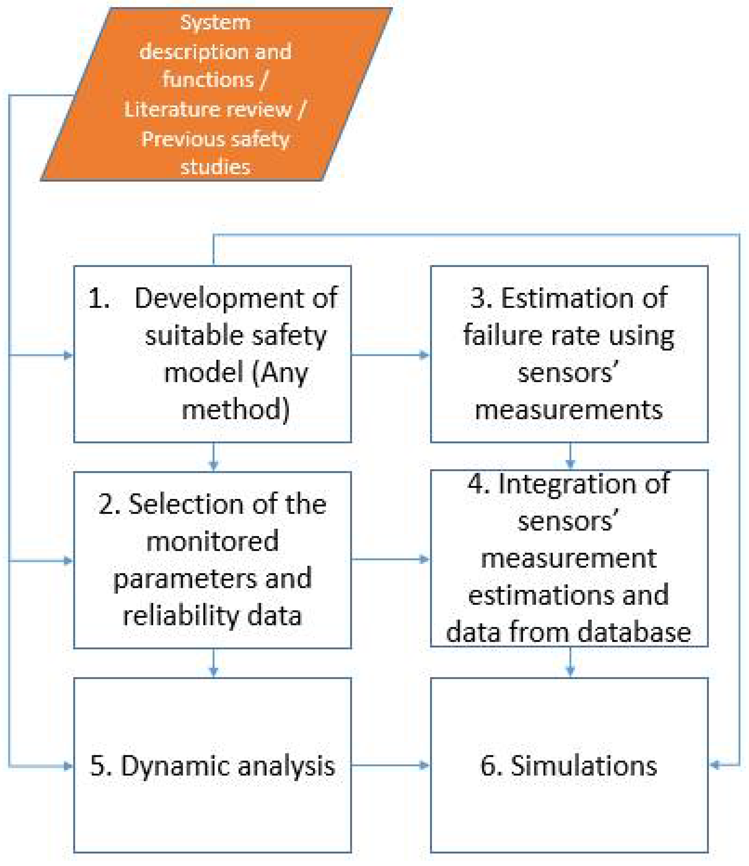
2.1. Methodology Overview

The general overview of the followed methodology for the development and validation of the proposed blackout monitoring system is provided in Figure 1. The first step includes the development of a safety model suitable for the blackout monitoring for the investigated cruise ship power plant system. In the second step, the parameters that can be monitored using sensors from the investigated cruise ship monitoring system are identified. During the third step, the failure rates of the investigated system components are estimated based on sensor measurements. In the fourth step, the methodology for fusion of selected system parameters/sensor measurements with the developed safety models and existing reliability data is presented. In the fifth step, criteria and metrics for the dynamic analysis of the observed situations are provided. In the sixth step, the system is simulated in a virtual environment and the concept is validated.

2.2. Step 1—Development of Safety Model

The first step of the methodology includes the development of a suitable safety model representing the system operation. In general, various safety analysis methods can be employed for this purpose including Fault Tree Analysis, Hazard and Operability studies, Bayesian Network [22], Boolean-Driven Markovian Processes [23]. Other methods/software tools could be also used, such as Hip-HOPs [24], COMPASS [25] or MADe [26,27,28] for automatically deriving the Fault Tree or Dynamic Fault Trees. This study employs the Combinatorial Approach to Safety Analysis (CASA) method, which is presented in [29,30,31]. The CASA method advantage is that it captures more accurately the dynamic and software-intensive character of cyber-physical systems compared to the classical Fault Tree Analysis [29]. On the other side, CASA results in a very extensive depiction of the system top-event and is labour-intensive. The other safety methods have several limitations. The Hazard and Operability studies do not relate the various independent hazardous events together, whilst there is no clear guidance for the development of Bayesian Networks. Methods such as Boolean-Driven Markovian Processes, Hip-HOPs, COMPASS, or MADe do not capture properly the software-intensive character of cyber-physical systems. Therefore, the use of fault trees developed by employing the CASA method is considered as advantageous for the safety analysis in diesel-electric power plants (DEP) system as reported in [30].

2.3. Step 2—Selection of the Monitored Parameters and Reliability Data

The following criteria are employed for selecting measured parameters for their integration with/inclusion to the developed automated safety monitoring system:

• Measured parameters that sufficiently and effectively depict/represent the actual system health based on the pertinent literature.
• Measured parameters that represent the system configuration and power demand, e.g., operating DG set(s).
• Measured parameters monitored by the existing ship alarm and monitoring system.
• Measured parameters from the ship plant critical components, as identified from previous safety analyses or accident investigation data.

In addition to the required measured parameters, a number of failure rates is also required based on their availability and the relevant databases. These failure rates are used in conjunction with the sensor measurements to estimate the components failure rate. The databases, such as OREDA [32], are selected based on their relevance to the system, availability, their trustworthiness, and publication date. The proposed blackout monitoring system also incorporates the maintenance inspection intervals and the actual inspection implemented for the components.

2.4. Step 3—Estimation of Failure Rates Using Sensors Measurements

For the components, the safety metrics of which are monitored using sensor measurements, Health Indexes ($H{I}_i$) are estimated to depict the performance and health status of the ith component [33,34,35,36]. The $H{I}_i$ is estimated according to the following equation:

$$H{I}_i=\{\begin{array}{c}0, if \frac{\left|F_i-F_{alarm}\right|}{\left|F_{alarm}-F_{norm}\right|}>1\\ 1, if \frac{F_i-F_{norm}}{F_{alarm}-F_{norm}}<0\\ \frac{\left|F_i-F_{alarm}\right|}{\left|F_{alarm}-F_{norm}\right|}, elsewhere\end{array}$$

(1)

where $F_i$ represents a feature of for the system ith component, $F_{alarm}$ is the feature value when the component fails (this can be the $F_i$ value of an activated component failure alarm), and $F_{norm}$ denotes the feature value under normal conditions (without faults). Features are variables indicative of the components health status [37]. The considered features ($F_i)$ can be the component temperature and/or the pressure, a parameter estimated based on vibration analysis, or a combination of physical parameters, which can be considered as a reliable representation of component health status. $F_i$ can be estimated based on the physical parameters monitored for a system component in real-time or at periodic times. In real applications, the calculation of HI must be updated each time a significant difference exists between the initial feature value and the observed average value calculated over a specific time window. This time window depends on each component failure mode related to specific $F_i$. Preferably, $F_i$ is a physical parameter monitored by the existing alarm and monitoring system.

According to Equation (1), the ith component is fully functional when $H{I}_i$=1; it fails when $H{I}_i$ = 0; whilst intermediate values of HI_i indicate degrading performance conditions of the ith component. In case $F_i$ exceeds the alarm limit $F_{alarm}$, it is also considered that the component is faulty and in case $F_i$ is far away from both $F_{alarm}$ and $F_{norm}$ not on the side of $F_{alarm}$, the component is considered as healthy. The $F_{norm}$ is defined the normal value of the $F_i$ that is observed during operation. Usually, this information can be retrieved from operation and maintenance manuals. Under real conditions, the $F_{norm}$ can vary depending on the desired output from a system, e.g., the engine load will affect the normal exhaust gas temperature; however, it is considered as static herein.

Based on the estimation of the components $H{I}_i$, in absence of any other information, it is assumed that the components failure rates (retrieved from used database) (${\lambda }_i$) can be updated, according to the following equation:

$${\lambda }_{i,m}={\lambda }_i^{H{I}_i}$$

(2)

The index $m$ depicts the failure rate estimated based on sensors measurements. The working assumption behind Equation (2) is that the closer the feature is to the alarm or failure threshold, the higher is the probability that failure will occur in the next time period. It is also expected that the relationship between time and $H{I}_i$ is exponential, as lower values of the component health index correspond to much lower component remaining useful life [38,39]. This can be viewed as rather a conservative approximation for the component fault growth trend. By using the $H{I}_i$ as the exponent in Equation (2), smoothness and exponential relationship in transition between normal and failure condition is ensured. In addition, the boundary conditions are satisfied, as elaborated in the next sentences. When $H{I}_i$ equals to 1, the ${\lambda }_{i,m}$ equals to the initial component failure rate $\left({\lambda }_i\right)$, which is the only available information at the beginning about the failure rate. The ith component is considered faulty when $F_i$ reaches rm limit is reached ($H{I}_i=0),$ which provides a failure rate according to sensor measurements equal to 1 h⁻¹.

2.5. Step 4—Integration of Sensor Measurements Estimation and Database Data

For integrating the component failure rate with the health status estimated from the measured data, the following equation is used to calculate the actual failure rate of the ith component, employing the weight $(w$) assigned by the user or expert to different information sources as proposed in [36]:

$${\lambda }_{i,A}={10}^{\left[w\log {\lambda }_{i,m}+\left(1-w\right)\log {\lambda }_{i,}\right]}$$

(3)

The logic behind Equation (3) is that the expert/user can have different trust levels in the information available from the various measurements (sensors) and historical databases. Full reliance on the measured parameters is denoted with w = 1, whereas w = 0 denotes not reliance on the measured parameters. The parameter w in this study is common to all the components, but it can be also become component specific; hence, it is denoted as w_i.

2.6. Step 5—Dynamic Analysis

The warning levels are determined using reference $p^{TE}$, where $p^{TE}$ denotes the probability of the top event. In this study, the reference $p^{TE}$ ($p_{REF}^{TE}$) is the geometrical mean for the orange level. The other warning levels are considered to have probability one or two levels higher or lower than the reference level. The use of logarithmic scale is employed, as the relationships in Equations (2) and (3) are exponential. This is also in line with maritime regulations, which recommend the separation of intolerable, tolerable and negligible risk based on logarithmic scale [40]. In this respect, the warning levels described in

Table 1. Warning levels.

Warning Levels	Range
Red	[$p_{REF}^{TE}$ × 5, $p_{REF}^{TE}$ × 50]
Orange	[$p_{REF}^{TE}$ × 0.2, $p_{REF}^{TE}$ × 5]
Yellow	[$p_{REF}^{TE}$ × 0.02, $p_{REF}^{TE}$ × 0.5]
Green	[$p_{REF}^{TE}$ × 0.002, $p_{REF}^{TE}$ × 0.05]

were developed. The reference $p^{TE}$ can be set based on statistics or using expert opinion.

Based on Table 1, the system levels, requiring intervention can be defined. The intervention is proposed to take place in the red or orange levels. The identification of safety enhancement actions during operations is supported by employing appropriate importance metrics. The importance metrics can be used to identify the most important potential failures and, therefore, to prioritise the rectification actions. The use of Birnbaum $I_j^B\left(t\right)$ and Fussel−Vesely $I_j^{FV}\left(t\right)$ importance metrics is employed herein, as these are extensively employed for importance analyses, and they are associated with a clear physical meaning. High values of the Birnbaum importance metric indicate components that significantly affect the Fault Tree top event probability. Therefore, these components degradation must be carefully monitored. $I_j^B\left(t\right)$ can be also used to assess the top event sensitivity to some operating parameters such as number of operating DG sets or DG sets load. The Fussel−Vesely importance metric can be used to identify the components whose failure most probably will occur and will lead to the blackout. Higher value of $I_j^{FV}\left(t\right)$ for a component, compared to other components, means that the top event will more likely occur from this component failure than from others.

The Birnbaum importance measure is estimated according to the following equation:

$$I_j^B\left(t\right)=\frac{\partial P^{TE}}{\partial p_{i,A}}\approx \frac{\Delta P^{TE}\left(p_{i,A}\right)}{\Delta p_{i,A}}\approx \frac{P^{TE}\left(p_{i,A}\right)-P^{TE}\left(p_{i,A}=0\right)}{p_{i,A}}$$

(4)

where $p_{i,A}$ is probability of the basic event calculated by using ${\lambda }_{i,A}$.

This study also adopted an alternative version of the Birnbaum importance metric that accounts for the plant operating parameters, such as engine load or number of connected DG sets. This metric is used to identify if a reconfiguration of the power plant is required to reduce the top event probability. Such reconfiguration may include the starting up of an additional DG set. This metric is calculated according to the following equation:

$$I_j^{B,OP}\left(t\right)=\frac{\Delta P^{TE}\left(OP\right)}{\Delta OP}\approx \frac{P^{TE}\left(OPinitial\right)-P^{TE}\left(OPfinal\right)}{SmallchangeinOPparameters}$$

(5)

The following measures are considered small changes in the operating parameters values ($\Delta OP$): reducing the number of operating DG by 1 unit, slightly increasing the DG set load, reducing the number of connected electrical power consumers.

An averaged over time $I_j^{Bt}$ metric is used to estimate the importance of each basic event in the Fault Tree based on the $I_j^B\left(t\right)$ values at different time steps and is estimated as follows:

$$I_j^{Bt}=\frac{1}{c{r}_{max}}{\displaystyle \sum }_{cr=1}^{cr=c{r}_{max}}{I}_j^B\left(t\right)$$

(6)

where $cr$ denotes an importance estimation number for the identified components, whereas $c{r}_{max}$ denotes the maximum number of implemented importance estimations. $I_j^{Bt}$ in this way is an averaged value of $I_j^B\left(t\right)$ and depicts the averaged criticality of a component.

The Fussel−Vesely importance measure is estimated by using the following equation:

$$I_j^{FV}\left(t\right)=\frac{\partial P^{TE}/P^{TE}}{\partial p_{i,A}/p_{i,A}}=\frac{p_{i,A}}{P^{TE}}\frac{\partial P^{TE}}{\partial p_{i,A}}\approx \frac{p_{i,A}}{P^{TE}}\frac{\Delta P^{TE}\left(p_i^{Agg}\right)}{p_{i,A}}\approx \frac{P^{TE}\left(p_{i,A}\right)-P^{TE}\left(p_{i,A}=0\right)}{P^{TE}}$$

(7)

An averaged over time $I_j^{FVt}$ metric is used to estimate the importance of each basic event based on the $I_j^{FV}\left(t\right)$ values at different time steps; this is estimated by the following equation:

$$I_j^{FVt}=\frac{1}{c{r}_{max}}{\displaystyle \sum }_{cr=1}^{cr=c{r}_{max}}{I}_j^{FV}\left(t\right)$$

(8)

The use of $I_j^{FVt}$ has similar purpose with $I_j^{Bt}$.

The importance measures indicate which components’ failures/operating parameters must be monitored and controlled. Based on that, recommendations for the system safety enhancement can be provided. Examples of such recommendations include the switching over to a healthier DG set (allowing for performing maintenance and repair actions to the degraded DG set), increasing the number of operating DG sets, or reducing the propulsion motors load (speed).

2.7. Step 6—Simulation in Virtual Environment

In this step, the relevant adjustments are implemented to the safety model developed in step 1 to allow for the dynamic estimation of $p^{TE}$ in a virtual environment. These adjustments are not implemented to the safety model structure, but to the basic nodes of the safety model and are delineated in

Table 2. Calculation of the basic events probabilities according to CASA and the in the performed simulations.

	System Components	Original Fault Tree Probability [30]	Modified Fault Tree Probability Estimation (Used for Simulation)
Operating components	Software, hardware, communication and sensors failures following exponential distribution for failure rate [41]	$p_{i,j}^{OC}={\lambda }_i$t	$p_{i,j}^{OC}={\lambda }_i\Delta t$
	Other components with preventative maintenance following Weibull distribution for failure rate	$p_{i,j}^{OC}={{\rm T}}_i^{{\beta }_i-1}{\lambda }_i^{{\beta }_j}t$	$p_{i,j}^{OC}={\beta }_j{\lambda }_i^{{\beta }_j}{t}_i^{{\beta }_i-1}\Delta t$
	Parts with preventive maintenance where a single component failure out of $r$ identical will lead to event occurence (based on [41])	$p_{i,j}^{OC}={\displaystyle {\displaystyle \sum }_1^r}\left(\begin{array}{c}r\\ 1\end{array}\right){\left({{\rm T}}_i^{{\beta }_i-1}{\lambda }_i^{{\beta }_j}\right)}^r{\left(1-{{\rm T}}_i^{{\beta }_i-1}{\lambda }_i^{{\beta }_i}\right)}^{1-r}t$	Replaced with OR gates connecting components failures. Each component failure rate is modelled by $p_{i,j}^{OC}={\beta }_j{\lambda }_i^{{\beta }_j}{t}_i^{{\beta }_i-1}\Delta t$
	Parts with preventive maintenance where all the $r$ identical components must fail for event occurrence (based on [41])	$p_{i,j}^{OC}=\left[{\left({{\rm T}}_i^{{\beta }_i-1}{\lambda }_i^{{\beta }_i}\right)}^r+r{{\rm T}}_i^{{\beta }_i-1}{\lambda }_i^{{\beta }_i}{\left(\frac{{\lambda }_i}{{\lambda }_i+{\mu }_i}\right)}^{r-1}+{\left(\frac{{\lambda }_i}{{\lambda }_i+{\mu }_i}\right)}^r\right]t$	Replaced with AND gates connecting components failures. Each component state is modelled as a Markov process, whereas each component failure rate is estimated by $p_{i,j}^{OC}={\beta }_j{\lambda }_i^{{\beta }_j}{t}_i^{{\beta }_i-1}\Delta t$
Safety systems	Tested standby equipment failure on demand (except for software failures) [41]	$p_{i,j}^{SS}=1+\frac{\left(e^{-{\lambda }_i{T}_i}-1\right)}{{\lambda }_i{T}_i}$	$p_{i,j}^{SS}=1+\frac{\left(e^{-{\lambda }_i{T}_i}-1\right)}{{\lambda }_i{T}_i}$
	For safety system/functions with continuous monitoring failure on demand [41]	$p_{i,j}^{SS}=\frac{{\lambda }_i}{{\lambda }_i+{\mu }_i}\left(1-e^{-\left({\lambda }_i+{\mu }_i\right){{\rm T}}_i}\right)$	Modelled as Markov process
	Safety functions with periodical testing failure on demand [41]	$p_{i,j}^{SS}=1+\frac{\left(e^{-{\lambda }_i{T}_i}-1\right)}{{\lambda }_i{T}_i}$	$p_{i,j}^{SS}=1+\frac{\left(e^{-{\lambda }_i{T}_i}-1\right)}{{\lambda }_i{T}_i}$
	For software failures in safety functions [41]	$p_{i,j}^{SS}=PF{D}_i$	$p_{i,j}^{SS}=PF{D}_i$
	Unavailability due to periodical maintenance of standby equipment where $r$ components are standby (based on [41])	$p_{i,j}^{SS}={\left(\frac{\raisebox{1ex}{$1$}\!\left/ \!\raisebox{-1ex}{$T_i$}\right.}{\raisebox{1ex}{$1$}\!\left/ \!\raisebox{-1ex}{$T_i$}\right.+{\mu }_i}\right)}^r$	Replaced with AND gate connecting components failures. Each component failure rate is estimated by Equation (8) and each component state is modelled as a Markov process.

. Some of the developed Fault Tree basic events from step 1 are transformed into the suitable Markovian process. This makes the developed Fault Tree similar to the Boolean-logic Driven Markovian Process (BDMP) [23]. The use of Markovian process has been considered as necessary to depict some dynamic features of the investigated system, which are not available in the Fault Tree. The required input for this step of the analysis includes the plant operational data, such as components in operation, components maintenance intervals and testing intervals ($T_i$), maintenance rates (${\mu }_i$), components failure rates (${\lambda }_i$), beta factor of the Weibull distribution (${\beta }_i$), and the probability of failure on demand for the software components ($PF{D}_i$). $\Delta t$ denotes the predicted time horizon at each time $t$.

The use of these equations constitutes an improvement to the CASA calculations, as they allow for estimating the selected safety metrics time variations, compared to the static predictions of the previously presented approaches [29,30].

For the simulation purposes only, it was assumed that the $F_i$ is calculated according to the following equation:

$$F_i=F_i^{norm}+F_i^{deg}\left(t-t_i^m\right)+noise$$

(9)

where $F_i^{norm}$ is the normal feature value, whilst $F_i^{deg}$ is degradation parameter, $t_i^m$ is the time of the last maintenance for the component $i$. A noise term is introduced in the analysis to account for the sensor’s measurement uncertainty. However, the actual fault growth curve can differ significantly from the proposed curve and depends on the component operating conditions. These assumptions are used only for the simulation purposes.

The $F_i^{deg}$ was assumed to be equivalent to the half of the inverse of the maintenance inspection interval. This assumption was made based on the observation that the preventative maintenance scheme in maintenance manuals quite often is implemented every half of the component useful life.

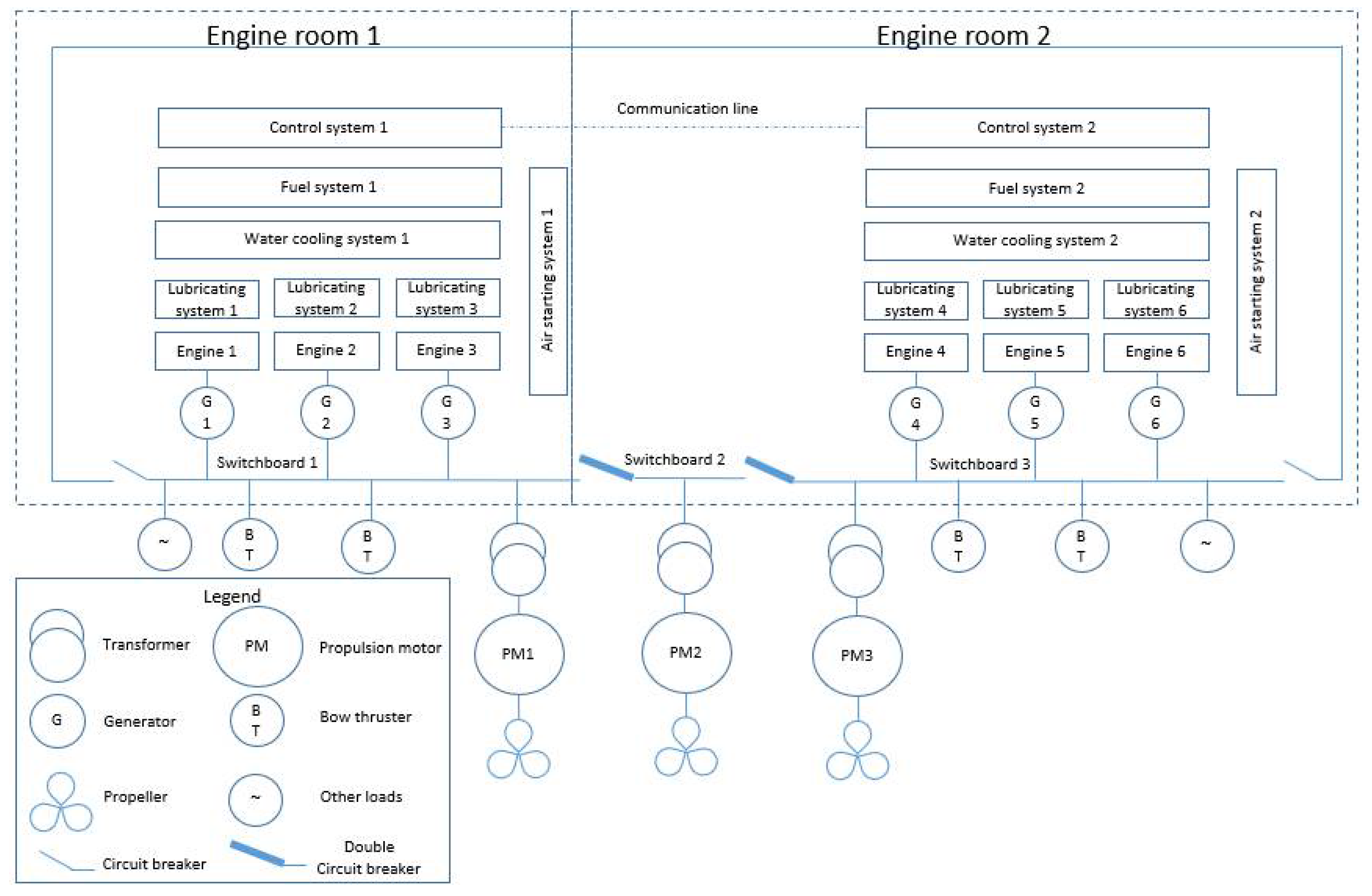
3. Investigated System Description

The investigated cruise ship diesel-electric power plant (DEP) includes 6 DGs, 3 azipods, 2 Power Management Systems (PMS) and 3 switchboards and multitude of other components as shown in Figure 2. Design data for this system was retrieved from the operating and maintenance manuals of the system components, the associated system drawings and studies published in the pertinent literature [42,43,44,45,46,47,48].

The instantaneous electric power demand affects the use (switching on/off) of the DG sets, whereas the DGs switchover is also implemented based on the DG sets accumulated running hours. The investigated system is capable of implementing fast load reduction of the propulsion electrical motors, and it also includes preferential tripping functions (fast load reduction) by tripping the electric motors driving the air conditioning system compressors. The engines of each DG set can be loaded till 90% of its nominal power. The ship electric load is evenly shared in proportion to the nominal power output of the DG sets among the operating DG sets. Prewarning alarms can allow a DG set to switch over to a healthy DG set, for example, in cases of lubricating oil low-pressure alarm, high exhaust gas temperature alarm and high cooling water temperature alarm are present. More detailed information about the investigated system can be found in [30].

The analysis and simulations require reliability and maintenance interval data for the components of the investigated power plant. However, this data sets were already presented in [30], and for reasons of brevity, are not provided herein.

Case Studies Description

The selected case studies are presented in

Table 3. Investigated case studies description.

Case Study No.	$\mathit{w}$	Analysis Conducted
1	0	Estimation of PoB every 0.5 h for 168 h (7 days, 1 week) with horizon prediction ($\Delta t)$ of 24 h
2	0.5	Estimation of PoB every 0.5 h for 168 h (7 days, 1 week) with horizon prediction ($\Delta t$) of 24 h and importance analysis every 24 h
3	1	Estimation of PoB every 0.5 h for 168 h (7 days, 1 week) with horizon prediction ($\Delta t)$ of 24 h

. The analysis employed different $w$ values to assess the impact of sensors measurements on the model results. The analysis focuses on the Probability of Blackout (PoB), denoted by $p^{TE}$. In addition to PoB, other metrics, such as the probability of sudden loss of a DG set (PoDGloss) is estimated, considering the basic events of the same Fault Tree model for estimation of PoB. The dynamic importance analysis is implemented for the case study 2 with w = 0.5 every 24 h to demonstrate the dynamic analysis results. The time horizon of 24 h was selected, as there have been some computational limitations identified in the implementation of importance analysis on smaller time steps. The PoB reference is set to 2.7 10⁻⁴ in line with published accident statistics and used in [30], whilst the PoDGloss is set to 0.1, so that the red zone geometric mean probability is equal to 1.

4. Results

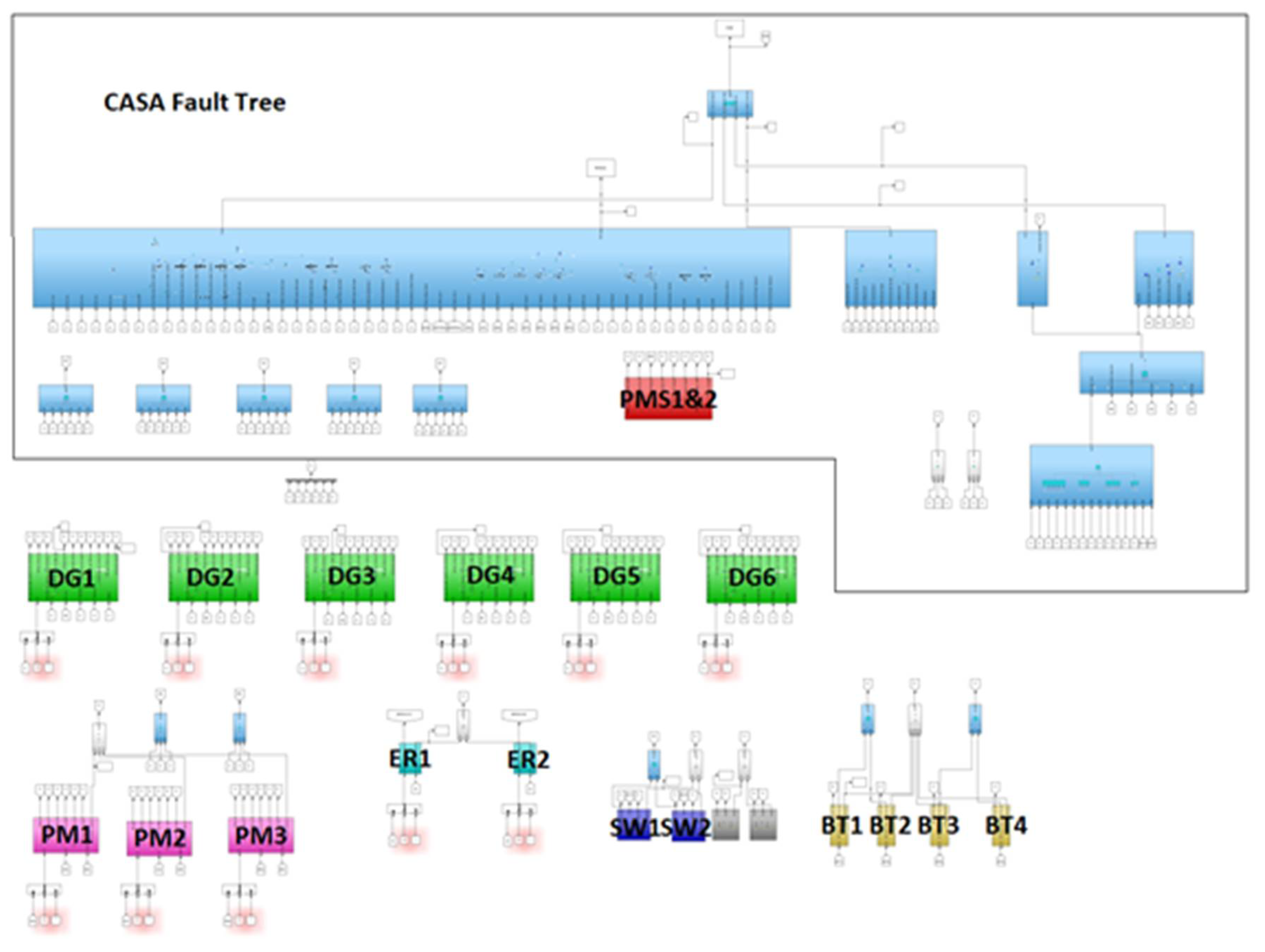
4.1. Step 1—The Developed Safety Model

The model has been developed for blackout monitoring system simulation in Matlab/Simulink environment by modelling all the relevant components, such as the major DEP subsystems: DG sets, Propulsion Motors (PM), Engine Room (ER) components, Bow Thrusters (BTs), Switchboards (SW). The basic event probability for each component as well as the components operating status are used in the Fault Tree calculations. The employed Fault Tree structure is not presented, as it is too extensive; detailed information about the developed Fault Tree model can be found in [30]. This Fault Tree calculates the safety metrics in a static manner. However, considering the implementation of the adjustments described in step 6, the developed model is capable of calculating the time variations of the selected safety metrics. This developed FT model interface in Simulink is provided in Figure 3.

4.2. Step 2—Selection of the Monitored Parameters

The features $F_i$ that were selected for the health monitoring of several components of the investigated system along with these components maintenance intervals (used to estimate $F_i^{deg}$) are provided in

Table 4. Selected features for the identified critical components of the investigated cruise ship power plant system.

a/a	Component	${\mathit{F}}_{\mathit{i}}$	Normal/Alarm Value	MI * (hours)
1	Engine Thrust bearings	Temperature	80/100 °C	18,000
2	Engine Main bearings	Temperature	80/100 °C	18,000
3	DG engine high temperature cooling water pump	Pressure at engine inlet	4/2 bar	10,000
4	DG set engine low temperature cooling water pump	Pressure at engine inlet	3.6/2 bar	10,000
5	Engine low temperature cooling water pump	Pressure	3.6/2 bar	10,000
6	Cylinders Exhaust gas	Temperature at exhaust gas port	450/490 °C	6000
7	Turbocharger (TC)	Temperature at turbine inlet	450/490 °C	12,000
8	Engine lubricating oil cooler	Temperature at engine inlet	70/80 °C	10,000
9	Lubricating oil pump	Pressure at engine inlet	4/3 bar	5000

* MI: Maintenance interval.

. These selected parameters are available in the existing ship alarm and monitoring system, and are typically employed for monitoring the safety critical components of the investigated power plant, as reported in [30].

Other parameters that are used as input to the FT model are: DG sets operating status, DG sets load, engine room operating status (whether in use or not; the ship has two engine rooms), number of operating DG sets in each engine room, hotel electric power demand, propulsion motors operating status and load, bow thrusters’ status and load, whether a DG set is starting, whether a propulsion motor is starting.

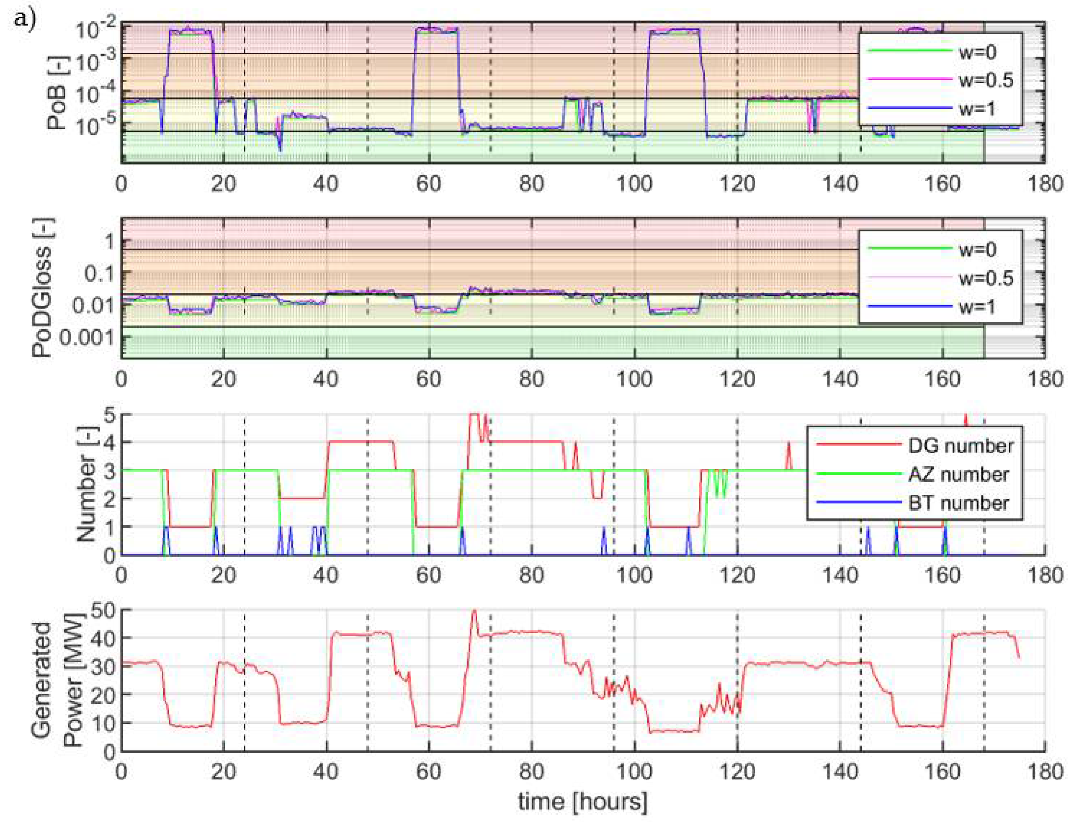
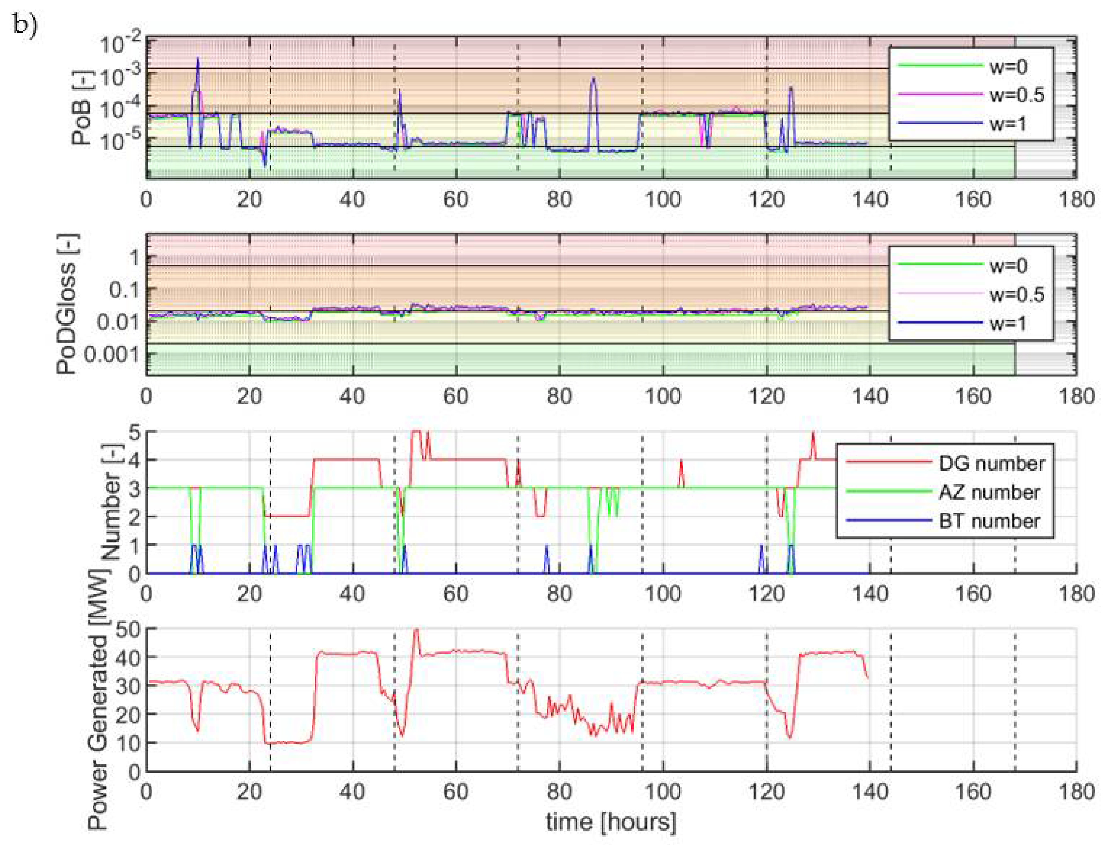
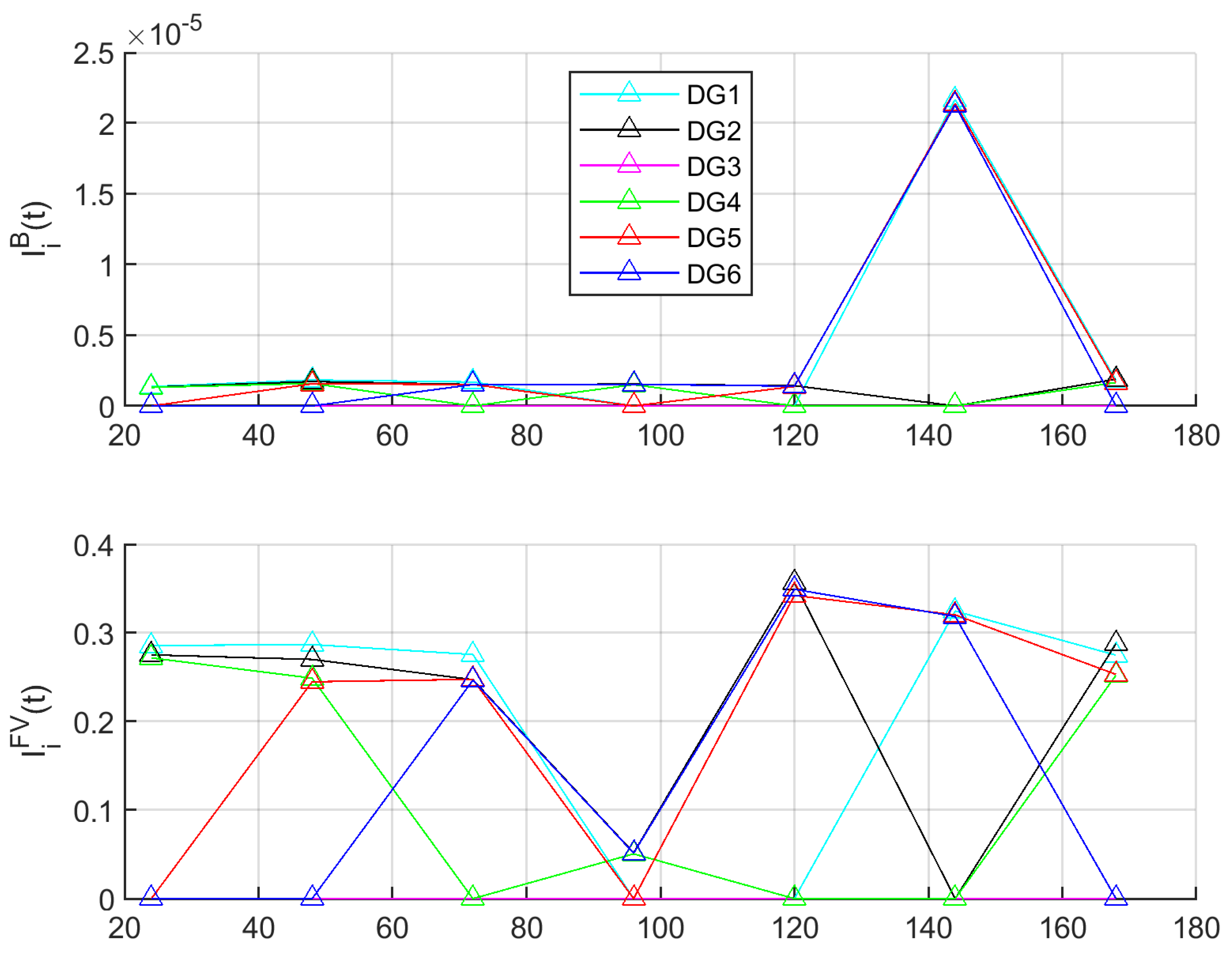
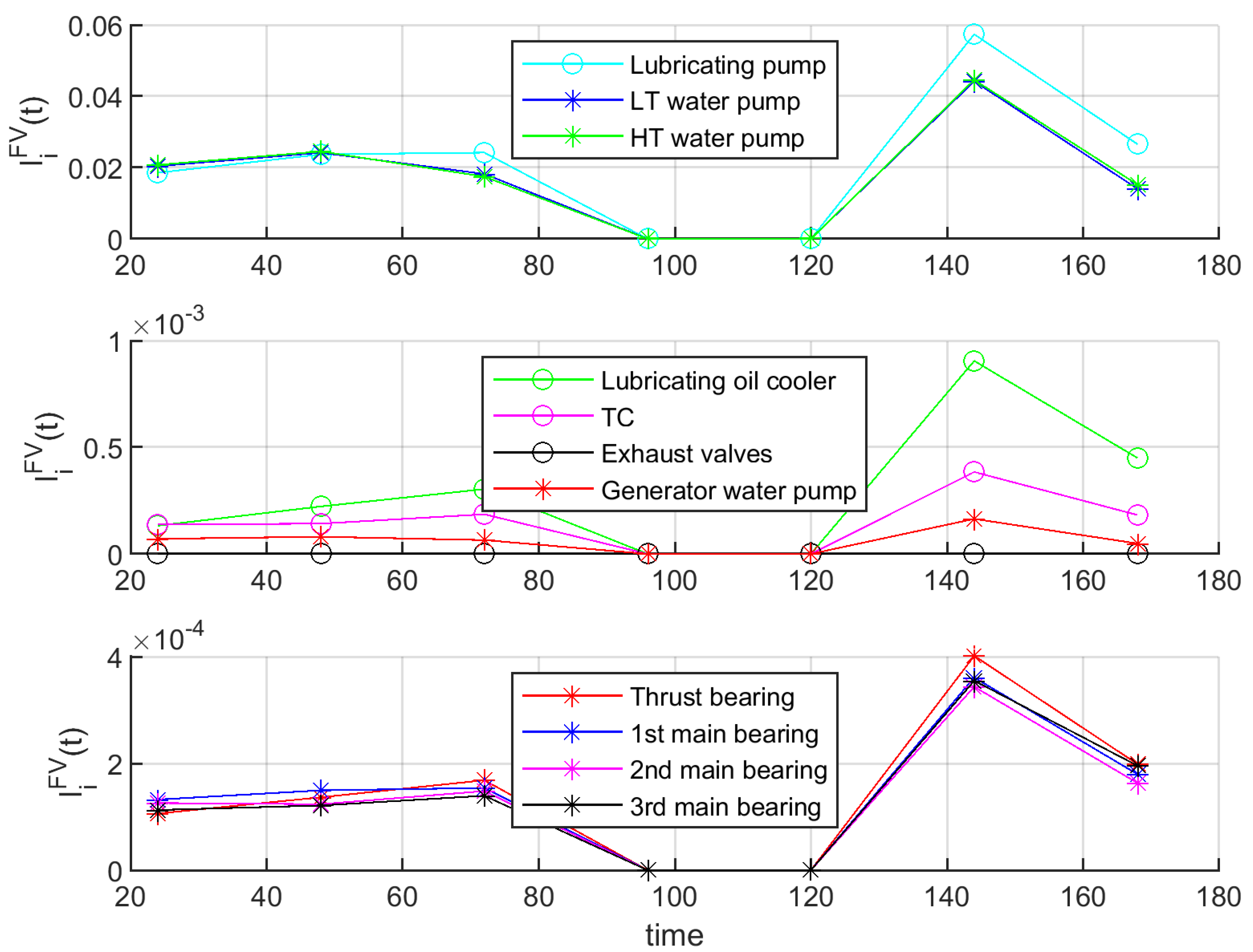
4.3. Steps 3−6—Simulation Results

Figure 4a illustrates the simulation results for the time variations of the power plant blackout probability and the probability of the sudden loss of one DG set for the three investigated case studies along with the numbers of the power plant main components (DG sets, azipods, bow thrusters) operating and the electric power demand time variation which are used as input. Therefore, the first two upper subplots of Figure 4a depict the output, whilst the two lower subplots depict the input. The inclusion of input and output is used to facilitate the identification of correlations between the input and output. Furthermore, to facilitate the results analysis, the same results are presented in Figure 4b, excluding the time periods in which one DG set operates.

As it can be observed from Figure 4a, the PoB is in red warning level for the time periods cases when only one DG set operates. At these time periods, the propulsion motors (azipods) do not operate, which indicates that the vessel is in the harbour mode. Therefore, it is deduced that the PoB significantly increases in harbour mode, which is aligned with findings of our previous study [30]. In this respect, the proposed system is developed to provide alarms for the cases where the warning zone is reached and the cruise ship operates in any mode.

The PoB is also exceeded for short time periods when the propulsion motors (azipods) do not operate and the ship operates in its manoeuvring mode using its bow thrusters; the electric power demand is relatively low, whilst three DG sets operate. This can be attributed to the fact that power reduction functions for the bow thrusters are not available, and hence, this safety barrier cannot be considered in this ship operating mode. It can be inferred that the power reduction functions have a critical role for reducing the PoB, and hence, in ensuring the ship safety, which is in alignment with findings from our previous study [30]. Thus, a potential way to improve the ship safety would be by including the power reduction functions for the bow thrusters, provided that the cruise manoeuvring operation is not jeopardised.

The probability of sudden loss of a DG set (PoDGloss) in the system is also presented in Figure 4. It is observed that the PoDGloss time variation follows the same pattern with the time variation of the connected (operating) DG sets number. This can be attributed to the fact that the more DG sets are connected to the system, the higher the probability that one of them will fail. However, the PoB seems to only slightly correlate to the PoDGloss, which indicates that other parameters are more critical for the PoB than the connected DG sets number, except for the time periods when only one DG set is connected. This indicate that the impact of this incidence (DG failure) is lower. These parameters are identified in the following paragraphs. The PoDGloss are generally in yellow region, which indicate that from this perspective, no intervention is required by the crew.

The three performed case studies employed different values of the weights (0, 0.5 and 1) to exclude, partly use, or only use the measured parameters for the calculation of the PoB time variations. It is deduced from the results of Figure 4 that differentiation of the PoB time variations are derived for these three case studies. This indicates that the incorporation of sensor measurements by the proposed blackout monitoring system influences the PoB results. This comparison is used to demonstrate the impact from incorporating the sensors’ measurements additionally on the components failure rates estimations. More importantly, the dynamic measurement of parameters (through sensors), such the number of connected components, their loading conditions, and others significantly influence the risk metrics estimation.

The derived importance measures for the selected components are provided in

Table 5. Importance measures results.

Component or Software Function Failure	${\mathit{I}}_{\mathit{i}}^{\mathit{B}\mathit{t}}[-]$	Type of Failure
Power Management System failure to reduce load of propulsion motors	0.0047	Software
Arc protection software failure	1.21 × 10−9	Software
Arc in switchboards N1 and N2	0.0072	Physical
DG 1 water cooler failure	0.0004	Physical
DG 1 Engine lubricating oil cooler	0.0004	Physical

and Figure 5 and Figure 6. These figures illustrate the importance measures calculated every 24 h, and consequently, the variation of these importance metrics in intermediate time steps is not provided. However, the provision of lines facilitates the results visualisation. The importance metrics in Table 5 are in alignment with the results reported in [30], and demonstrate that not only physical failures but also failures in software functions are categorised as critical for system safety. Additionally, the derived results demonstrate the importance of other hazardous events, e.g., arc in switchboards. Based on the preceding considerations, the system operator must pay attention to measured parameters variation and the degradation of the identified critical components and failures, as small changes in these parameters can have significant influence on the power plant PoB.

It is deduced from Figure 5 that the importance metric for each DG set varies with time. It must be noted that for the cases where a DG set is not connected to the ship electric grid (does not operate), its importance metric equals to 0. The importance metrics variation depends on the usage of the DG sets and operating loads, the system configuration and the components degradation. DG2, DG5 and DG6 exhibit a relatively low value of the importance metric $I_i^{FV}\left(t\right)$ at t = 96 h, as three DG sets operate at relatively low load; thus, it is unlikely that a failure in one of these operating DG sets will result in blackout. Therefore, it can be inferred that it would be possible to operate at this time period with only two DG sets at a higher load, which is expected to improve the energy efficiency of the investigated power plant, with only slightly affecting the plant safety (in terms of the PoB). The considerable values of the importance metric $I_i^B\left(t\right)$ for DG1, DG5 and DG6 at t = 144 h demonstrated a higher sensitivity of these operating DG sets to failures. This indicates situations where the crew must be alerted for potential failures or degradation of the operating DG sets’ health status, as explained in the next paragraph.

Figure 6 provides the importance metrics $I_i^{FV}\left(t\right)$ for different components of DG1. These importance metrics time variations are related to the identified critical components operational characteristics, failure rates and degradation patterns. The most critical components for the DG1 operations were found to be the pumps for the lubricating oil as well as the cooling water of high and low temperature. These components require attention from the crew for DG1.

4.4. Discussion

From the results analysis of the preceding section, it has been demonstrated that the investigated power plant parameters, such as, the number of the operating DG sets connected to the ship electric grid, the power plant components’ health status, the DGs’ operating conditions (load), affect the system safety. To address the power plant safety issues during operation requires to account for all these parameters, which complicates the decision-making process for assuring the system safety. However, with an assistance from proper tools for analysing pertinent information, these parameters effects can be quantified and used to estimate the safety metrics for the investigated power plant, allowing for the identification and treatment of potentially hazardous conditions more effectively. With the development of autonomous systems in the maritime industry and the replacing of human operations by smart systems, such monitoring tools are essential for ensuring the systems safety. In the context of fully autonomous ships, the presence of advanced and intelligent safety monitoring systems is prerequisite.

The proposed concept for the development of the presented blackout monitoring system satisfies several criteria for automating the power plant safety monitoring and management [12]. It provides high-level functional alarms for the investigated cruise ship power plant based on the prevailing system operating conditions. It also allows for the classification of the alarms/failures to reflect their importance on the investigated power plant safety. Furthermore, it allows the operator to assess indirectly the impact of different failures on the ship functions and to select the components that need to be maintained or disconnected from the ship electric grid. Therefore, it can be inferred that this concept facilitates the effective safety management for the power plants of cruise ships.

Nonetheless, the proposed monitoring system has some limitations. A future study could focus on diagnostics development and use of the shipboard measurements to develop diagnostics toolboxes. Prognostics algorithms could be also incorporated in the blackout monitoring system. Future study could also investigate the impact of different maintenance and inspection intervals on the power plant safety. Methods for diagnosing the sensor failures and measurements uncertainty could also further enhance the propose monitoring system functionality. However, the presented concept constitutes the first essential step to the development of a fully automated blackout monitoring system.

5. Conclusions

This study proposed a novel blackout monitoring system for the power plant of a cruise ship. This system integrates a Fault Tree model developed through CASA method with sensor measurements and reliability data for the system components. The system calculated the time variations of the investigated plant safety metrics, in specific the probability of blackout and the probability to loss a DG set. Real operational data were used for performing simulations to validate the proposed concept.

The main findings of this study can be summarised as follows.

• Specific operational parameters as DG load and number of connected DG sets need be used as input into the safety monitoring system, as these influence the system’s probability of failure.
• An operation with a single DG set increases the PoB to the red warning level.
• The PoB during start of DG sets also reaches the red level.
• Failures in operating components can increase the PoB also above the desired threshold, however their criticality is varying in time dependent on the system other parameters.

This study demonstrated the usefulness and advantages of the proposed monitoring system considering that the power plant safety metrics depend on a diverse set of parameters varying in time. The concept as presented in this study is an effort towards the development of the proposed system, which is expected to benefit the cruise ship industry as well as other shipping sectors employing complex power plants and propulsion systems. It is also anticipated to be an essential tool for monitoring and management the dynamic safety metrics and risk for the case of autonomous ship systems.

References

1. Asariotis, R.; Benamara, H.; Finkenbrink, H.; Hoffmann, J.; Lavelle, J.; Misovicova, M.; Valentine, V.; Youssef, F. Review of Maritime Transport, 2011; United Nations: Geneva, Switzerland, 2011; ISBN 9211128412. [Google Scholar]
2. Cruise Lines International Association. 2017 Cruise Industry Outlook. 2016. Available online: https://cruising.org/-/media/research-updates/research/featured/2017-clia-state-of-the-industry.pdf (accessed on 1 December 2017).
3. Nilsen, O.V.; Johansen, C.B.; Knight, M.; Hoffman, P.; Skjong, R. FSA for Cruise Ships—Task 4.1.1—Hazid Identification; SAFEDOR-4.1.1 2005-12-31 DNV rev. 1; Det Norske Veritas, 2005; Available online: http://www.safedor.org/resources/SAFEDOR-D-04.01.01-2005-10-31-DNV-HAZID-Cruise-vessels.pdf (accessed on 1 June 2018).
4. MAIB. Report on the Investigation of the Catastrophic Failure of a Capacitor in the Aft Harmonic Filter Room on Board RMS Queen Mary 2 While Approaching Barcelona 23 September 2010; MAIB: Southampton, UK, 2011. [Google Scholar]
5. Ullah, Z.; Waldrop, T.; Chavez, N. Helicopters Sent to Rescue 1300 Passengers from Cruise Ship Off Norway. Available online: https://edition.cnn.com/2019/03/23/europe/norway-cruise-ship-evacuation/index.html (accessed on 30 September 2019).
6. DNV. Guidance for Safe Return to Port Projects; DNV GL: Hovik, Norway, 2016. [Google Scholar]
7. Bolbot, V.; Theotokatos, G.; Bujorianu, L.M.; Boulougouris, E.; Vassalos, D. Vulnerabilities and safety assurance methods in Cyber-Physical Systems: A comprehensive review. Reliab. Eng. Syst. Saf. 2019, 182, 179–193. [Google Scholar] [CrossRef] [Green Version]
8. DNV. 2025 Technology Outlook; DNV: Hovik, Norway, 2015. [Google Scholar]
9. Stefani, A. An Introduction to Ship Automation and Control Systems; Institute of Marine Engineering, Science & Technology: London, UK, 2013. [Google Scholar]
10. Malone, T.; Kirkpatrick, M.; Mallory, K.; Eike, D.; Johnson, J.; Walker, R. Human Factors Evaluation of Control Room Design and Operator Performance at Three Mile Island-2; Essex Corp: Alexandria, VA, USA; Washington, DC, USA, 1980. [Google Scholar]
11. Accident Investigation Boar Norway. Interim Report on the Investigation into the Loss of Propulsion and Near Grounding of Viking Sky; Accident Investigation Board Norway: Lillestrøm, Norway, 2019. [Google Scholar]
12. Papadopoulos, Y.; McDermid, J. Automated safety monitoring: A review and classification of methods. Int. J. COMADEM 2001, 4, 14–32. [Google Scholar]
13. Xing, J.; Zeng, Z.; Zio, E. A framework for dynamic risk assessment with condition monitoring data and inspection data. Reliab. Eng. Syst. Saf. 2019, 191, 106552. [Google Scholar] [CrossRef] [Green Version]
14. Hu, J.; Zhang, L.; Ma, L.; Liang, W. An integrated method for safety pre-warning of complex system. Saf. Sci. 2010, 48, 580–597. [Google Scholar] [CrossRef]
15. Hu, J.; Zhang, L.; Ma, L.; Liang, W. An integrated safety prognosis model for complex system based on dynamic Bayesian network and ant colony algorithm. Expert Syst. Appl. 2011, 38, 1431–1446. [Google Scholar] [CrossRef]
16. Aizpurua, J.I.; Catterson, V.M.; Papadopoulos, Y.; Chiacchio, F.; Manno, G. Improved Dynamic Dependability Assessment Through Integration with Prognostics. IEEE Trans. Reliab. 2017, 66, 893–913. [Google Scholar] [CrossRef] [Green Version]
17. Aizpurua, J.; Catterson, V.; Papadopoulos, Y.; Chiacchio, F.; D’Urso, D. Supporting group maintenance through prognostics-enhanced dynamic dependability prediction. Reliab. Eng. Syst. Saf. 2017, 168, 171–188. [Google Scholar] [CrossRef] [Green Version]
18. Gomes, J.P.P.; Rodrigues, L.R.; Galvão, R.K.H.; Yoneyama, T. System level RUL estimation for multiple-component systems. In Proceedings of the 2013 Annual Conference of the Prognostics and Health Management Society, New Orleans, LA, USA, 14–17 October 2013; pp. 74–82. [Google Scholar]
19. Pattison, D.; Segovia Garcia, M.; Xie, W.; Quail, F.; Revie, M.; Whitfield, R.; Irvine, I. Intelligent integrated maintenance for wind power generation. Wind Energy 2016, 19, 547–562. [Google Scholar] [CrossRef] [Green Version]
20. Abaei, M.M.; Hekkenberg, R.; BahooToroody, A. A multinomial process tree for reliability assessment of machinery in autonomous ships. Reliab. Eng. Syst. Saf. 2021, 210, 107484. [Google Scholar] [CrossRef]
21. Eriksen, S.; Utne, I.B.; Lützen, M. An RCM approach for assessing reliability challenges and maintenance needs of unmanned cargo ships. Reliab. Eng. Syst. Saf. 2021, 210, 107550. [Google Scholar] [CrossRef]
22. ISO. Risk management—Risk assessment techniques. In ISO 31010; International Organization for Standardization: Geneva, Switzerland, 2009; p. 92. [Google Scholar]
23. Bouissou, M.; Bon, J.-L. A new formalism that combines advantages of fault-trees and Markov models: Boolean logic driven Markov processes. Reliab. Eng. Syst. Saf. 2003, 82, 149–163. [Google Scholar] [CrossRef]
24. Kabir, S.; Papadopoulos, Y.; Walker, M.; Parker, D.; Aizpurua, J.I.; Lampe, J.; Rüde, E. A Model-Based Extension to HiP-HOPS for Dynamic Fault Propagation Studies. In Model-Based Safety and Assessment; Springer: Cham, Switzerland, 2017; pp. 163–178. [Google Scholar]
25. Bozzano, M.; Cimatti, A.; Katoen, J.-P.; Nguyen, V.Y.; Noll, T.; Roveri, M. The COMPASS approach: Correctness, modelling and performability of aerospace systems. In Proceedings of the International Conference on Computer Safety, Reliability, and Security, Hamburg, Germany, 15–18 September 2009; pp. 173–186. [Google Scholar]
26. Dionysiou, K.; Bolbot, V.; Theotokatos, G. A functional model-based approach for ship systems safety and reliability analysis: Application to a cruise ship lubricating oil system. Proc. Inst. Mech. Eng. Part M J. Eng. Marit. Environ. 2021. [Google Scholar] [CrossRef]
27. Milioulis, K.; Bolbot, V.; Theotokatos, G. Model-based safety analysis and design enhancement of a marine LNG fuel feeding system. J. Mar. Sci. Eng. 2021, 9, 69. [Google Scholar] [CrossRef]
28. Niculita, O.; Nwora, O.; Skaf, Z. Towards Design of Prognostics and Health Management Solutions for Maritime Assets. Procedia CIRP 2017, 59, 122–132. [Google Scholar] [CrossRef]
29. Bolbot, V.; Theotokatos, G.; Boulougouris, E.; Psarros, G.; Hamann, R. A novel method for safety analysis of Cyber-Physical Systems—Application to a ship exhaust gas scrubber system. Safety 2020, 6, 26. [Google Scholar] [CrossRef]
30. Bolbot, V.; Theotokatos, G.; Boulougouris, E.; Psarros, G.; Hamann, R. A Combinatorial Safety Analysis of Cruise Ship Diesel–Electric Propulsion Plant Blackout. Safety 2021, 7, 38. [Google Scholar] [CrossRef]
31. Bolbot, V.; Theotokatos, G.; Vassalos, D. Using system-theoretic process analysis and event tree analysis for creation of a fault tree of blackout in the Diesel-Electric Propulsion system of a cruise ship. In Proceedings of the International Marine Design Conference XIII, Helsinki, Finland, 10–14 June 2018; pp. 691–699. [Google Scholar]
32. OREDA. Offshore Reliability Data Handbook, 6th ed.; OREDA Participants: Hovik, Norway, 2015. [Google Scholar]
33. Knutsen, K.; Manno, G.; Vartdal, B. Beyond Condition Monitoring in the Maritime Industry; DNV GL Strategic Research & Inovation Position Paper; DNV GL: Hovik, Norway, 12 September 2014. [Google Scholar]
34. Jürgensen, J.H.; Godin, A.S.; Hilber, P. Health index as condition estimator for power system equipment: A critical discussion and case study. CIRED-Open Access Proc. J. 2017, 2017, 202–205. [Google Scholar] [CrossRef] [Green Version]
35. Bohatyrewicz, P.; Płowucha, J.; Subocz, J. Condition Assessment of Power Transformers Based on Health Index Value. Appl. Sci. 2019, 9, 4877. [Google Scholar] [CrossRef] [Green Version]
36. Aizpurua, J.I.; Stewart, B.G.; McArthur, S.D.; Jajware, N.; Kearns, M. Towards a hybrid power cable health index for medium voltage power cable condition monitoring. In Proceedings of the 37th IEEE Electrical Insulation Conference, Calgary, AB, Canada, 16–19 June 2019. [Google Scholar]
37. Goebel, K.; Daigle, M.; Saxena, A.; Sankararaman, S.; Roychoudhury, I.; Celaya, J.R. Prognostics the Science of Prediction; Create Space Independent Publishing Platform: Charleston, SC, USA, 2017; p. 396. [Google Scholar]
38. Hafver, A.; Pedersen, F.B.; Jakopanec, I.; Oliveira, L.; Domingues, J.; Eldevik, S.; Lindberg, D.V. Dynamic RISK Management for Enhanced Safety; DNV GL AS: Høvik, Norway, 2017. [Google Scholar]
39. Mutunga, J.M.; Kimotho, J.K.; Muchiri, P. Health-Index Based Prognostics for a Turbofan Engine using Ensemble of Machine Learning Algorithms. J. Sustain. Res. Eng. 2019, 5, 50–61. [Google Scholar]
40. EMSA. Risk Acceptance Criteria and Risk Based Damage Stability. Final Report, Part 1: Risk Acceptance Criteria. 2015. Available online: http://emsa.europa.eu/about/308-management/2419-study-1-emsa-3-risk-acceptance-criteria-and-risk-based-damage-stability-part-1-part-2.html (accessed on 1 June 2020).
41. Schüller, J.; Brinkman, J.; Van Gestel, P.J.; Van Otterloo, R. Methods for Determining and Processing Probabilities: Red Book; Committee for the Prevention of Disasters: Arnhem, The Netherlands, 1997. [Google Scholar]
42. Ådnanes, A.K. Maritime Electrical Installations and Diesel Electric Propulsion; ABB: Oslo, Norway, 2003; p. 86. [Google Scholar]
43. Kongsberg. Power Management System. Available online: https://www.km.kongsberg.com/ks/web/nokbg0397.nsf/AllWeb/B759133464F70B12C1256DEB0039EBCD/$file/AD-00447B_PMS_datasheet.pdf?OpenElement (accessed on 1 June 2017).
44. Radan, D. Integrated Control of Marine Electrical Power Systems. Ph.D. Thesis, Norwegian University of Science and Technology, Trondheim, Norway, 2008. [Google Scholar]
45. MAN. Diesel-Electric Propulsion Plants; MAN, 2012. [Google Scholar]
46. Krogseth, I.B. Dynamic Fault-Detection in Shipboard Electric Load Sharing; Norwegian University of Science and Technology: Trondheim, Norway, 2013. [Google Scholar]
47. Meyle. Arc Detection System. Available online: http://www.meyle.com.cn/pdf/arc-detection-systems.pdf (accessed on 1 September 2017).
48. Sfakianakis, K.; Vassalos, D. Design for safety and energy efficiency of the electrical onboard energy systems. In Proceedings of the 2015 IEEE Electric Ship Technologies Symposium, Washington, DC, USA, 21–24 June 2015; pp. 150–155. [Google Scholar]
49. AUTOSHIP. Autonomous Shipping Initiative for European Waters. Available online: https://www.autoship-project.eu/ (accessed on 1 January 2020).
Figure 1. Methodology flowchart for the development and verification of safety monitoring system.
Energies 14 06598 g001
Figure 2. Cruise ship propulsion system layout adopted from [30].
Energies 14 06598 g002
Figure 3. Cruise ship Fault Tree.
Energies 14 06598 g003
Figure 4. Derived time variations of PoB and probability of DG loss; (a) complete set of the investigated conditions; (b) Filtered set of operating conditions excluding the time periods where one DG set operate.
Energies 14 06598 g004aEnergies 14 06598 g004b
Figure 5. I i B ( t ) and I i F V ( t ) for the connected DG sets (horizontal axis is in hours). (Note: importance measures points are connected with lines for facilitating the results visualisation.).
Energies 14 06598 g005
Figure 6. I i F V ( t ) for different components of DG1 (horizontal axis is in hours). (Note: importance measures points are connected with lines for facilitating the results visualisation.).
Energies 14 06598 g006