Utilization of Two Sensors in Offline Diagnosis of Squirrel-Cage Rotors of Asynchronous Motors

Abstract

In the manufacture squirrel-cage rotors of asynchronous motors, a high standard of quality is required in every part of the production cycle. The die casting process usually creates porosity in the rotor bars. This most common defect in the rotor often remains hidden during the entire assembly of the machine and is usually only detected during final testing of the motor, i.e., at the end of the production process. This leads to unnecessary production costs. Therefore, the aim is to conduct a continuous control immediately after the rotor has been cast before further processing. In our paper, we are interested in selecting a suitable method of offline rotor diagnostics of an asynchronous motor that would be effective for these needs. In the first step, the selection of the method and its integration into the overall manufacturing process is carried out. The arrangement of the sensors and their calibration is then simulated on a 2D Finite Element Model of the rotor. The proposed offline measurement procedures and technologies are finally validated by testing measurements on a rotor that simulates the most frequently occurring faults. A test system is also developed that provides the operator continuous information about the running rotor measurements and makes it easier to evaluate the quality of the cast rotor by means of graphical visualization of the faults.

1. Introduction

In the production of asynchronous machine rotors, we often encounter the need to test their manufacturing quality during production. This type of testing can detect a production defect in the rotor early on, immediately after the rotor has been cast and removed from the die casting mold. Otherwise, this defect would only appear at the end of the manufacturing process of the electric motor during its output testing [1,2]. In this case, the motor is still repairable by total rotor replacement. This method adds enormous extra manufacturing costs. Moreover, a complete rotor replacement is very difficult to perform in the mass production of electric machines. Additional costs are incurred in all the technological operations that the rotor goes through after casting. These include the pressing of the shaft into the stator pack, the adjustment of the rotor dimensions and its surface, the overall balancing of the rotating masses, the pressing of the bearings onto the shaft, and its final fixing to the frame with the stator [2].

Rotor manufacturing failures can be divided into two categories according to the significance of the failure: major and minor [3,4]. Major defects can be detectable by the naked eye or by using image processing [5,6,7]. These include broken bars, bars separated from the rings, bulging material on the rotor surface, or completely missing material in the ring or bar. Minor defects in cast rotors are mainly caused by air bubbles in the bars and end-rings or internal material deformation caused by intensive cooling of the molten metal [8]. A rotor with such defects may seem visual to be perfectly fine, but from an electrical view, it has reduced resistance, which may be unevenly distributed between the bars and end-rings [8,9]. In the case of die-cast rotor cages, where the rings are in direct contact with the rotor packing, visual inspection even by an experienced technician may be unsuccessful and minor defects practically undetectable [2,4].

The internal shape of the rotor bars and their overall arrangement can also be very varied, e.g., single straight bars, skewed bars, and single or double cage rotors. The shape of arrowed rotor bars with a middle ring is also often found [10,11]. The rotor slots can be open, semi-closed, or fully closed [12,13,14]. The variability of the rotors, in general, makes the identification of failures difficult and is quite insufficient in multi-series production of cast rotors.

During several decades, very high-quality methods have been developed and elaborated, which are today commonly used to identify machine failures based on online diagnostics [15,16,17,18,19,20]. These methods are useful during operation when disassembly of the electric motor is not required. Fault measurements can be performed at a safe distance from the machine [21]. Widely used techniques are, e.g., single-phase test with reduced machine supply, MSCA (Motor Signature Current Analysis), or diagnostics from the stray field in radial or axial direction [21,22]. Although these methods can detect minor rotor faults, such a system is not suitable for diagnosing a single rotor after casting because it requires a machine stator. In an assembled machine, the test results can also be affected by the condition of other motor components such as the stator, its magnetic circuit with windings, bearings, etc. [23,24].

To detect failures in the squirrel-cage rotor immediately after die casting, it is necessary to search in an off-line test group that does not include any motor components other than the rotor itself. In this area, we can find, for example, magnetic foil diagnostics, dye penetrant, DLRO (Digital Low Resistance Ohmmeter) measurements, or ultrasonic measurements to determine the quality of the end-rings [25]. There also exists a method that requires high current excitation (HCE) in which local hot spots on the rotor surface are measured using an IR camera. The temperature can reach high values and the flowing currents can distort the measuring equipment [3,4].

The Growler test is historically the oldest off-line method of measuring rotor quality. It was originally used for winding rotors of commutator machines to locate inter-turn connections or interrupted connections of the winding outputs to the commutator [26]. The Growler yoke excites an AC magnetic field in the rotor, which induces a voltage in the bars (windings). When a part of the winding is interrupted or short-circuited, a local change in the magnetic field is produced on the rotor surface. The change in the field can be detected by ferromagnetic identification tape, magnetic foil, Hall sensor, or by comparing the change in supply current as of the rotor slowly rotates. For best sensitivity, the rotor is usually in direct contact with the poles of the Growler yoke [27].

Other methods use direct analysis of the magnetic field response or measurement of the magnetic induction value near the rotor surface to test the rotor. The rotor usually rotates at a slow speed during the measurement and the excitation magnetic field is generated by an external source using a core coil or permanent magnets [28,29]. Here, the rotor defect is represented by a reduced or missing magnetic flux amplitude. Direct magnetic measurements have their indisputable advantages, but the technology used is quite expensive and requires a good quality measurement system with fast converters. Additionally, Hall probes are very fragile to handling and there is a risk of mechanical damage in normal technological operation.

The main motivation is to find and choose a suitable off-line method of rotor diagnostics. Overall, the diagnostic system should be simple and located in the rotor manufacturing process between the die casting technology and the following operations before the assembly with the stator. From the reference literature used [28,30], it is more or less evident that the main evaluation method for the identification of rotor defects is the currently used FFT analysis. Especially in the case of the use of FFT analysis, the diagnostic post in the manufacturing company needs to be covered by a researcher or a person with a higher qualification. However, such a solution is not possible in mass production of rotors. This led us to the idea of trying to visualize the defect of the tested rotor in a different way than the above mentioned procedures. The main aim of our work is to provide the information about the defect of the manufactured rotor to the operator so that the identification of the defect is based on a graphical pattern. In addition, the literature [28,30] also show the outputs of practical implementation of measurement systems that can be used in practice in mass production of rotors. However, there is no detailed discussion of the use of 2-sensor measurements, which we believe can provide new information in rotor diagnostics.

The paper is organized as follows. In Section 2, the finding of a suitable technique for off-line rotor diagnostics is described and the arrangement of sensors for measuring rotor defects is proposed. The design of the sensors is also described. In Section 3, a numerical simulation of a 2D electromagnetic model of the rotor is performed and the overall functionality of the proposed measurement system is validated. In Section 4, the construction of a test rotor designed to simulate rotor faults is described. In Section 5, the processing of the sensor signals, their handling, and analysis is described. In Section 6, measurements on a real rotor of an asynchronous motor are made and validation of the measurement results is performed. The discussion and conclusion is presented in Section 7 and Section 8.

2. Sensor Configuration and Measurement Method

From the point of view of simplicity, reliability, and sensitivity, a sensor whose basic principle is based on Faraday’s law of electromagnetic induction was considered for rotor diagnostics [31]. The magnetizing yoke that generates the static magnetic field is located near the rotor [28,29]. The magnetic field lines from the excitation yoke are closed by an air gap across the rotor teeth around the rotor bar slots. When the rotor rotates, a voltage is induced in the rotor bars. All the bars are short-circuited at both end-rings and then current flows through the rotor bars. This current creates its magnetic field and affects the original excitation static field.

The generated response in the magnetic field will also produce a time change in the magnetic flux. This change is detected and a voltage is induced in the sensing coil. A healthy rotor generates a regular periodic voltage waveform, while a defect rotor shows a deformation in the voltage waveform depending on the type of fault. The magnitude and shape of this voltage are therefore in direct proportion to the physical state of the rotor [30]. In the search for a suitable arrangement, several possible designs and sensor arrangements were selected, see Figure 1.

Figure 1a shows a sensor excited by a DC current source, Figure 1b shows a sensor where excitation is provided by permanent magnets glued to the poles of the sensor’s magnetic circuit, and finally Figure 1c shows a variant with a permanent magnet on one pole of the sensor. In all cases, the magnetic sensor circuit was made in a U-shape to simplify the handling of the sensing coil. Although such sensors are quite simple to manufacture, we found a number of problems when aligning them to the rotor. These active sensors showed a high tendency to vibrate due to the pulsating magnetic pull as the rotor rotates.

To eliminate the vibrations transferred to the sensing part of the sensor, we partially separate the excitation and sensing functions by dividing the sensor into 2 pieces, active and passive. The active sensor contains excitation permanent magnets NdFeB type N42. Its sensing coil is placed longitudinal between the pole extensions and wound on an insulating core frame. The coil contains approximately N = 150 turns of insulated wire and is oriented in the axis of rotation. The pole extensions and the core of the sensing coil are assembled from high grade oriented electrotechnical sheet M165-35. The active sensor assembly is clamped with brass screws between aluminum holders, see Figure 2.

The passive sensor in Figure 2 consists of a magnetic circuit also made of oriented sheets and bent into a U-shape. Two sensing coils are attached to its poles. Each of the coils contain approximately N = 500 turns of insulated wire and the two coils are electrically connected in series to increase the value of the induced voltage. The passive sensor assembly is fixed in a non-magnetic insulating enclosure.

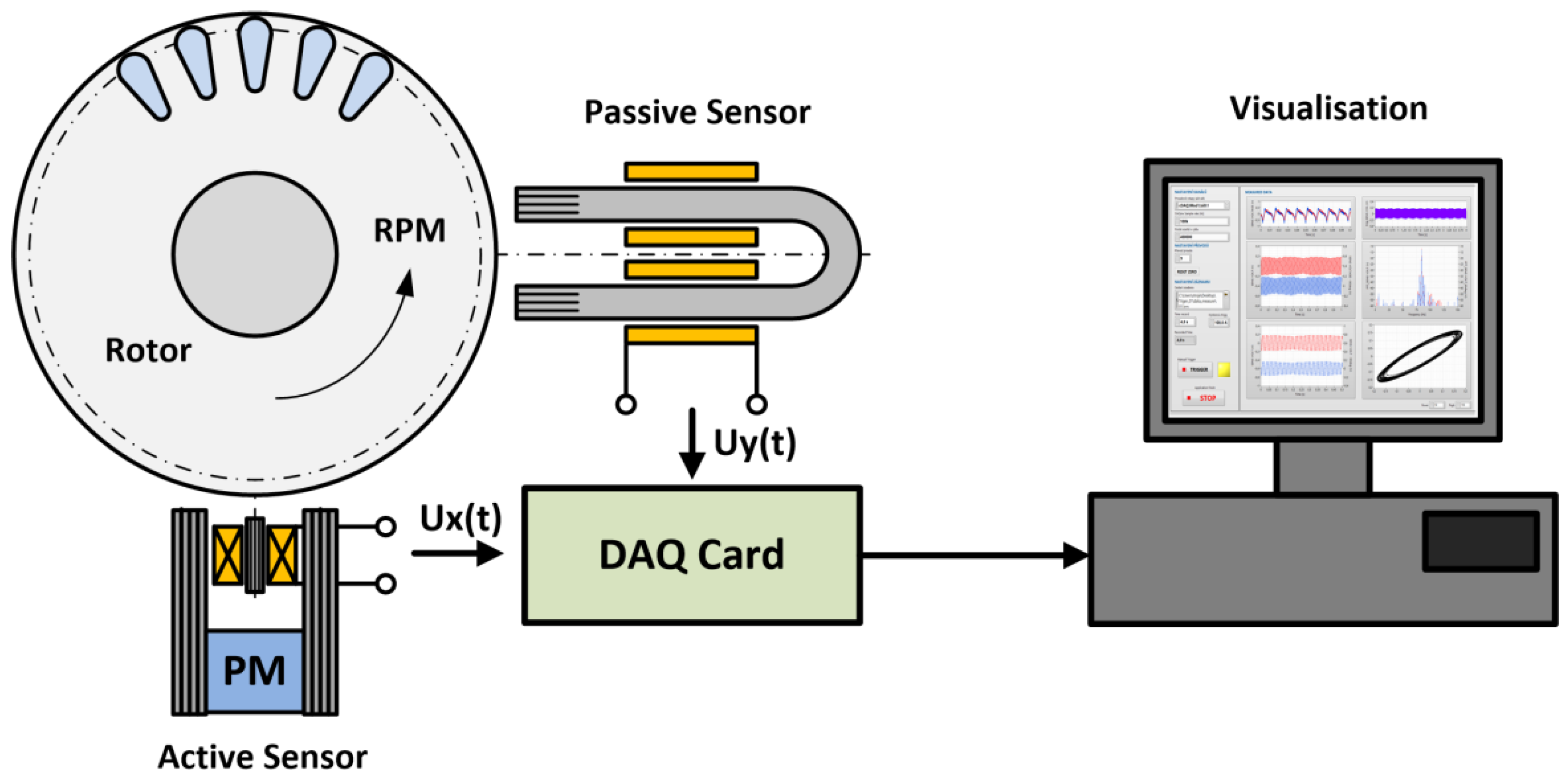
The configuration of the measurement system shown in Figure 3 was found to be the most convenient from a practical point of view. Identification of rotor faults uses a combination of active and passive sensors rotated 90 deg relative to each other. The active sensor generates the necessary static magnetizing field and senses its change as the rotor rotates. The passive sensor captures the stray field near the rotor surface.

The voltage outputs of both sensors are fed to a DAQ card connected to a computer. The measured voltages are then adjusted, amplified, filtered, and processed by software. The modified signals are then analyzed and displayed graphically for the operator to evaluate.

3. 2D FEM Electromagnetic Simulation

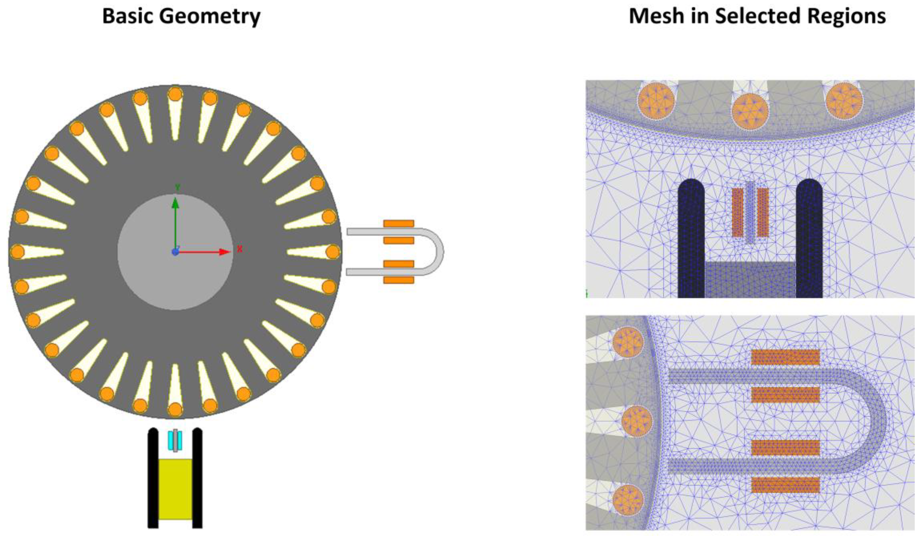
A 2D FEM electromagnetic model was used as a basic tool to verify the functionality of the designed rotor measurement system. In the initial phase, the FEM model was used to find the most suitable arrangement of sensors and to determine their optimal positions and dimensions. The FEM model contains a rotor sheet with slots in which the rotor bars are placed in isolation, see Figure 4.

The active sensor is located at the bottom, while the passive sensor is located on the right along the direction of rotor rotation. In the air gap and rotor bar regions, the model is built with a precision mesh to eliminate false induced voltage waveforms due to poor discretization. The FEM model contains approximately 60,000 elements and transient time analysis was used to solve the model.

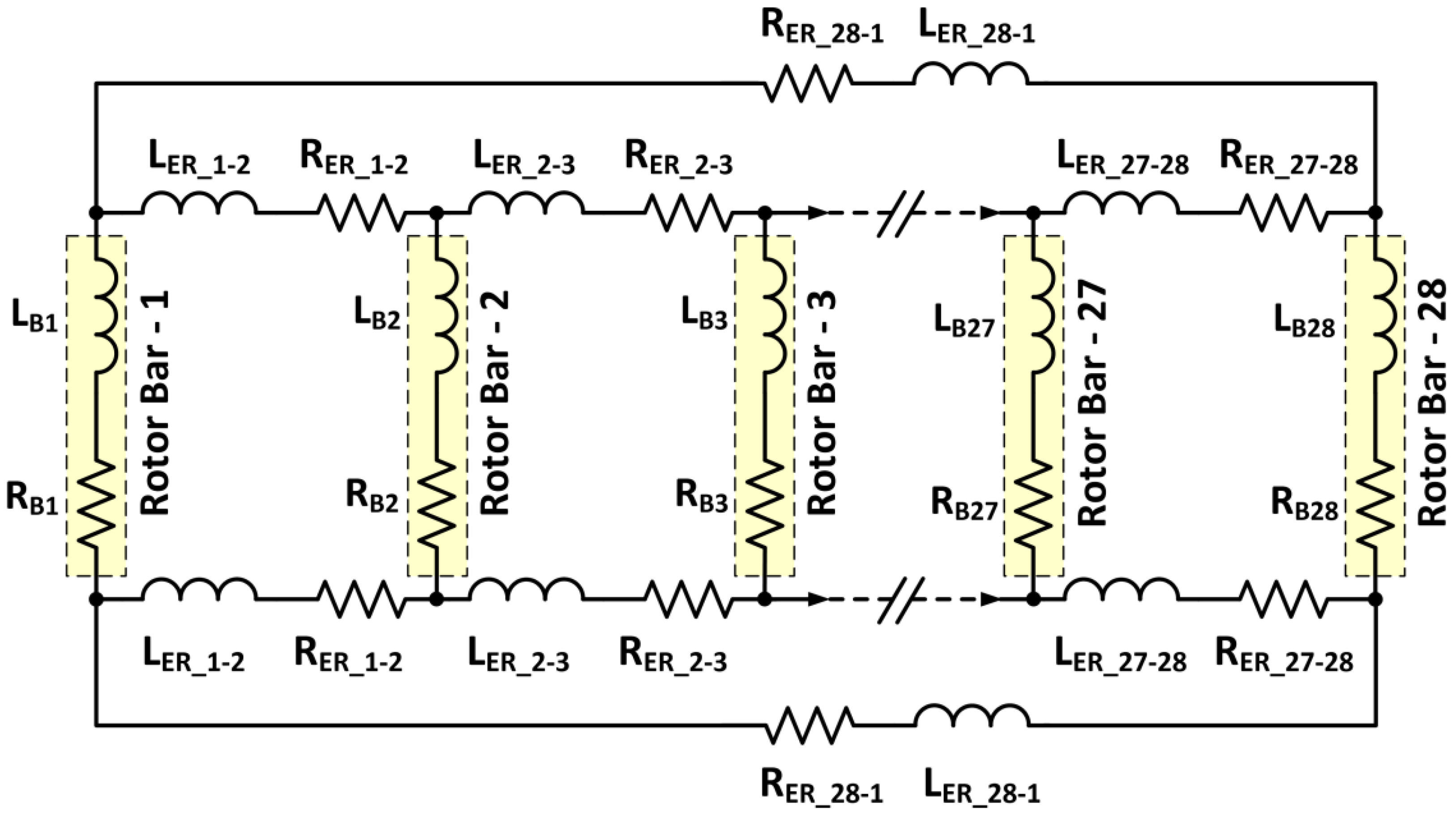
The electromagnetic model was solved in Ansys Maxwell, which also allows to define an external electrical circuit with a direct link to the electromagnetic FEM model. The external circuit was used to describe the squirrel cage of the rotor, see Figure 5.

The circuit diagram is fully enclosed and consists of inductances and resistances. The circuit elements are arranged to represent the electrical coupling of the rotor bars (Rbx, Lbx) with the end-ring segments (Rer_xy, Ler_xy) [32,33]. By changing the values of the circuit elements, the characteristics of the bars and end-rings can be described in the case of a simulated fault, e.g., a broken bar, a ring segment with reduced conductivity, or overall a combination of faults.

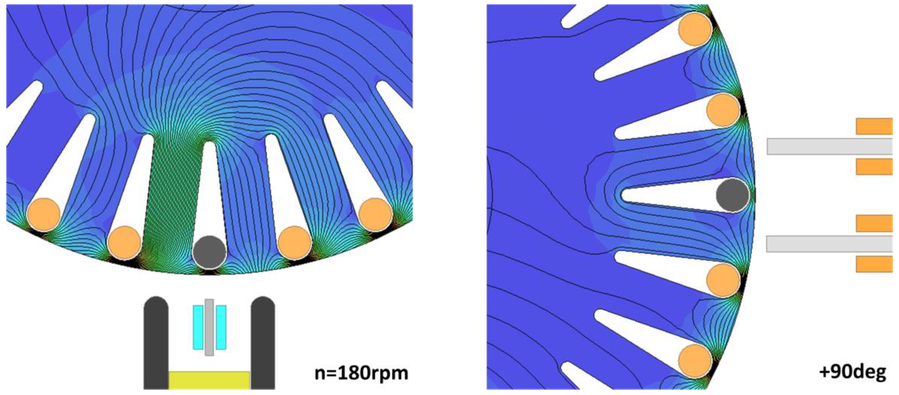
As the rotor rotates, the currents in the bars create a reaction field that distorts the originally symmetrical field of the magnetization yoke. Figure 6 shows the magnetic field distribution in the rotor as the faulty bar passes by the two sensors.

The faulty bar is shown here in black color. No voltage is induced in this broken bar and the current value Ibar = 0 A. No reaction flux is then generated in the surroundings of the bar and a part of the magnetic flux passes through the adjacent tooth. At this point, a deformation occurs in the total magnetic field, which is captured by the sensing coil of the active sensor and also by the coil of the passive sensor.

When the rotor is rotated by 90 deg, the broken bar reaches the passive sensor. Here, the magnetic flux lines are locally closed through a region across the rotor teeth that surround the faulty bar and the contact bridge of the closed slot. This local distortion of the magnetic flux reappears in the stray field and is again detected by the passive sensor.

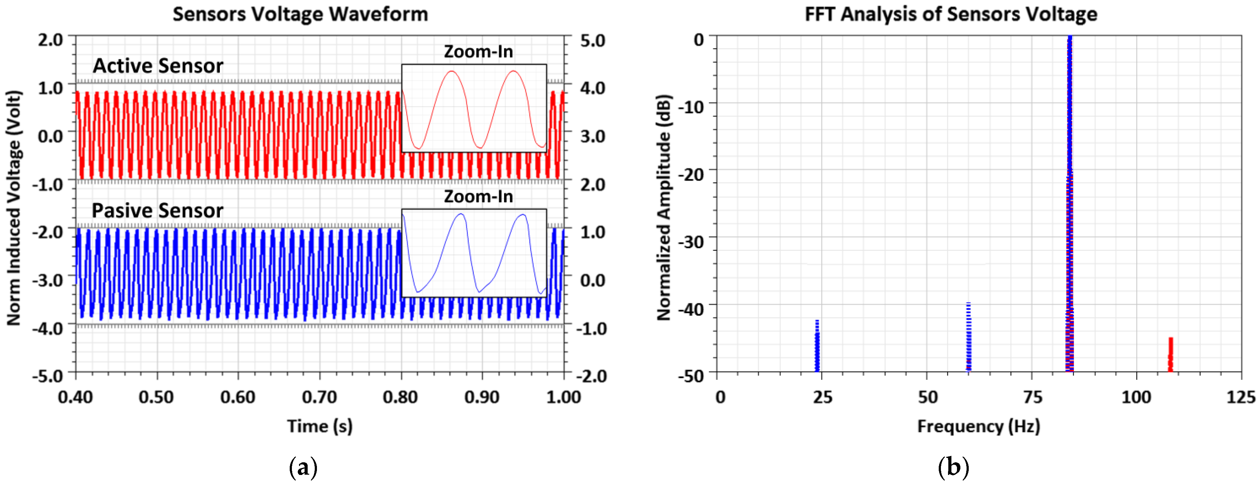
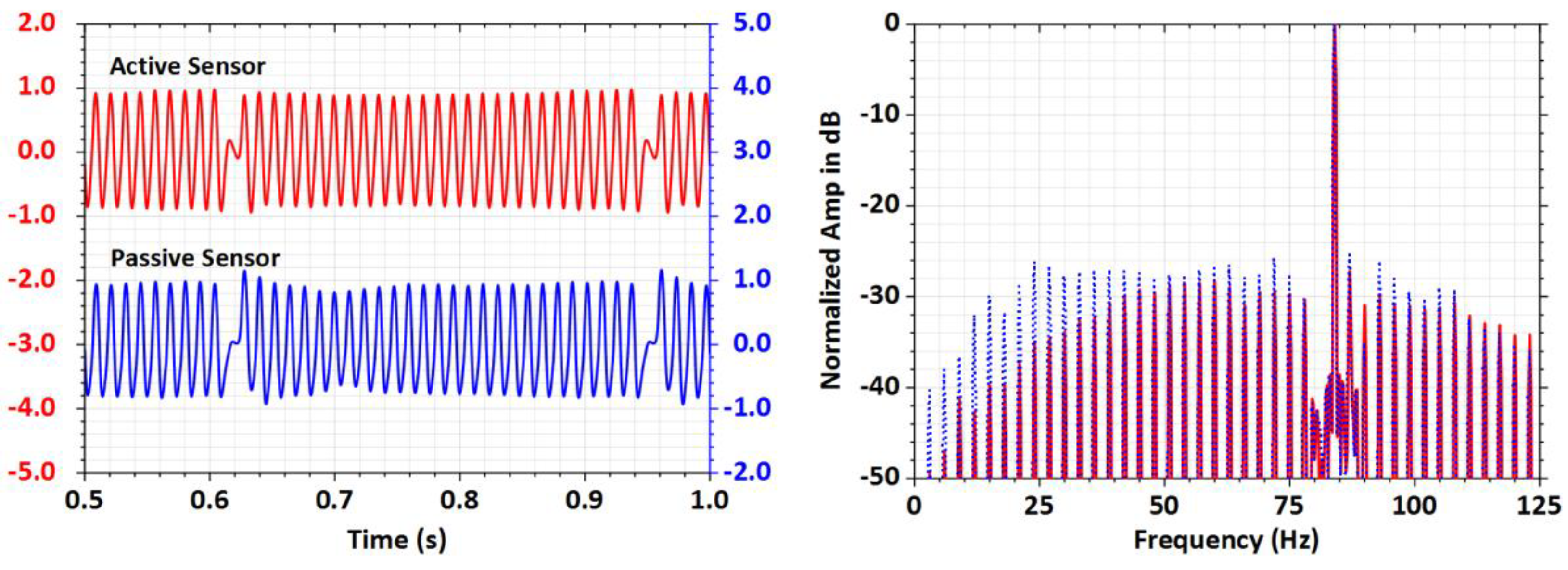
The induced voltage waveforms on the sensing coils of the active and passive sensors of the FEM model are shown in Figure 7a. A time window t = (0.4–1.0) s is selected for plotting, where the voltage waveforms are in steady state already. The waveforms are offset in the graph to avoid overlapping and to make them clearer. The red color corresponds to the induced voltage of the active sensor, the blue color to the induced voltage on the passive sensor. The voltage range of both signals is also normalized in the interval (−1,1). The time waveform of both voltages is not pure sinusoidal but shows a shape deformation. The deformation is more visible in the voltage waveform of the passive sensor. A healthy rotor without defects shows a regular waveform of both induced voltages without deviations. Figure 7b shows the FFT analysis of both sensor signals. The normalized amplitude spectrum is shown, where the frequency fx = 84 Hz visibly dominates. The value of this frequency corresponds to the set rotor rotation speed n = 180 rpm and the number of its slots (bars) Ndr = 28. The sidebands also appear and do not exceed the value of −40 dB in amplitude. The sidebands are much more significant in a passive sensor.

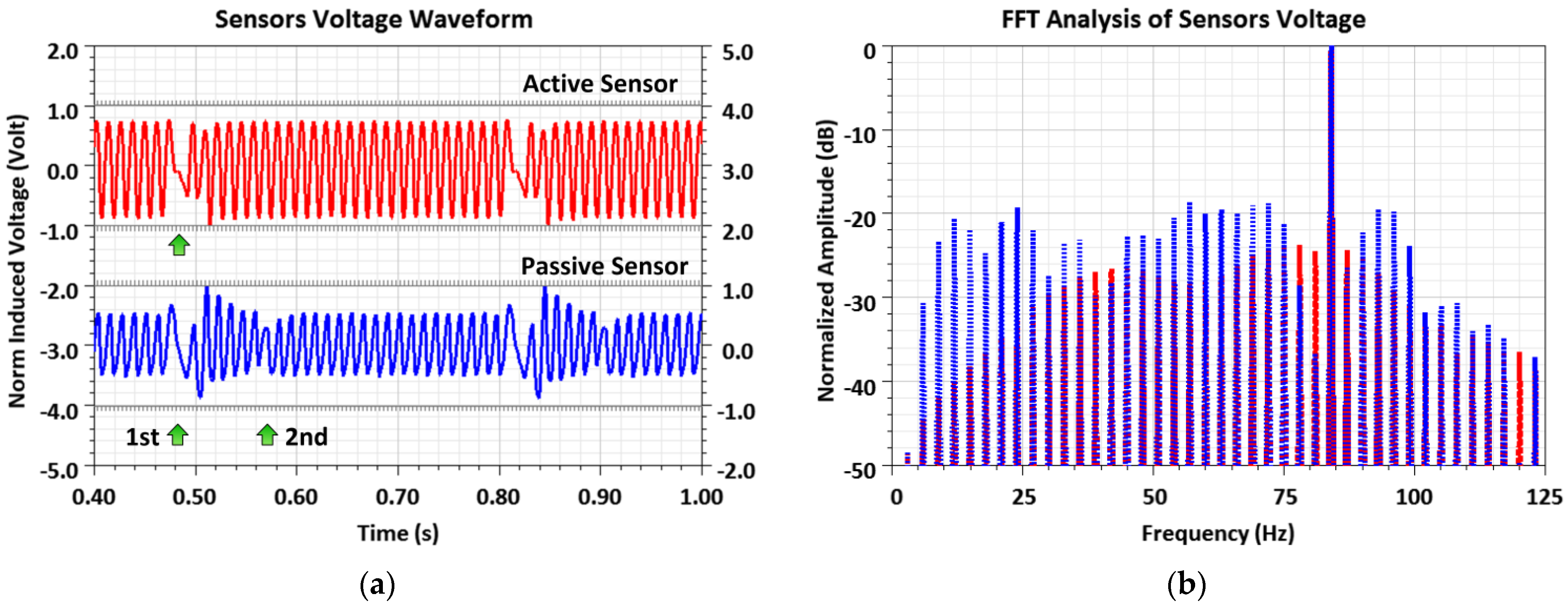
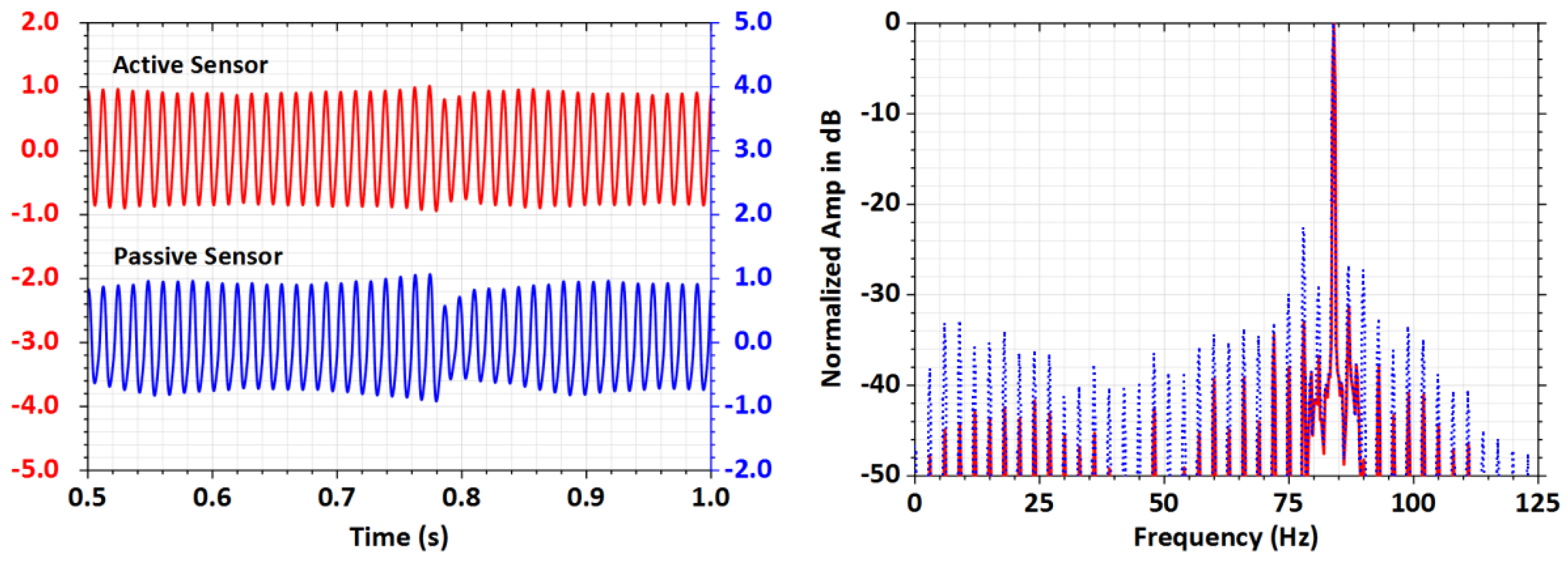
Figure 8a shows the induced voltage waveforms for the FEM simulation of 1 broken bar. There is a region on the induced voltage waveform of the active sensor where part of it is completely missing (green arrow). This empty region is periodically repeated at the same time intervals as the rotor rotates. This indicates a fault in the bar, where the voltage is induced, but no electric current flows through the bar due to the missing electrical connection to the end-ring. The lack of a reactive magnetic flux will create a significant distortion in the otherwise regular voltage waveform on the active sensor. On the voltage waveform of the passive sensor, the information about the broken rotor bar appears at the same time point as for the active sensor (t1 = 480 ms). However, the voltage waveform is different on the passive sensor due to its different design nature. With a time delay of about Δt = 85 ms (in time t2 = 565 ms), the information about the broken bar reappears by the oscillation of the induced voltage on the passive sensor. This is the point at which the broken bar is close to the passive sensor and the rotor has rotated 90 deg (+7 bar displacement).

Figure 8b shows the FFT analysis of the voltages of both sensors. In addition to the main harmonic fx = 84 Hz, there are significant sidebands with a frequency separation of Δf = 3 Hz indicating a bar fault. For the active sensor, the signal offset is approximately −24 dB. The passive sensor is more sensitive due to the two detected distortions and the offset from the main harmonic is less than −18 dB.

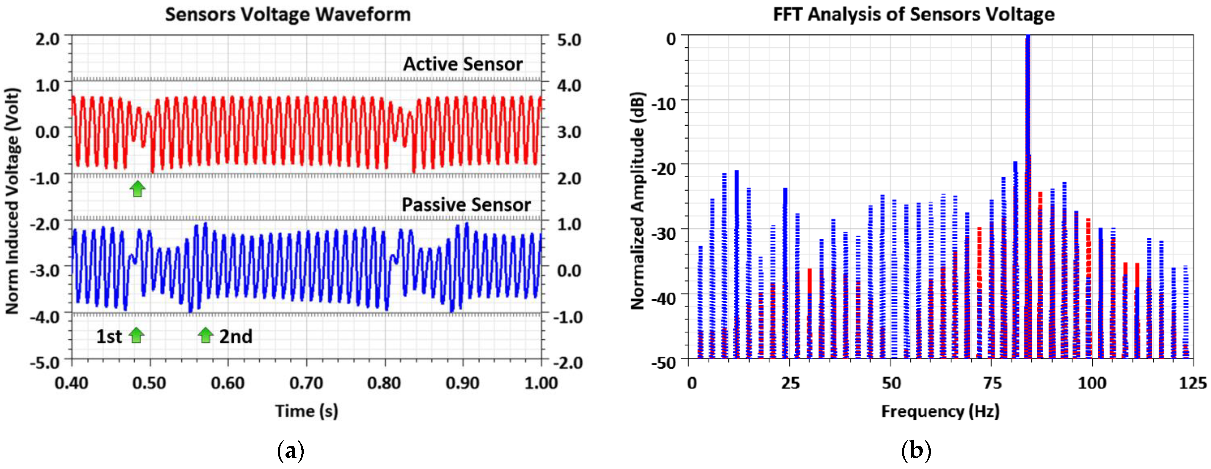
In the FEM simulation of a broken end-ring segment between the bars, this defect again presents similarly on both sensor induced voltage waveforms. It can be seen in Figure 9a that the broken segment between the bars causes multiple oscillations just as it passes over the excitation poles of the active sensor. The waveform is then further deformed in time by the DC component.

A segment failure is repeatedly visible on the induced voltage waveform of the passive sensor, similar to the case of a broken bar. The information about the faulty segment is at the same time instant as for the active sensor (t1 = 480 ms). It appears as an oscillation and a significant waveform distortion. Then, the amplitude of the oscillation decreases and then slowly increases until the faulty segment (2 adjacent bars with a faulty segment) is close to the passive sensor. Here again, the amplitude of the induced voltage increases suddenly (t2 = 565 ms). Figure 9b shows the FFT analysis of the voltages of both sensors. With the main harmonic fx = 84 Hz, significant sidebands with frequency spacing Δf = 3 Hz appear. For the active sensor, the sideband is concentrated around the main harmonic and also around the frequency f2 = 28 Hz, which corresponds to the number of rotor slots. In a passive sensor, the sidebands are distributed over the entire displayed frequency range (0–125 Hz). The lowest value of the offset signal is in the order of −21 dB.

The 2D FEM numerical model describes the problem only in the plane of the rotor section and thus is not able to provide all the relevant information, such as the rotor slot skew, the distribution of defects in the bar along the length, the axial rotation of the sensors, etc. The FEM simulation of the induced voltage waveforms on the sensors showed that the basic principle of the designed inductive sensors works reliably. The measurement system is able to detect a wide range of rotor manufacturing defects with sufficient resolution. With the help of the performed electromagnetic field simulations, the optimum locations for sensor placement were found and also the optimization of the active and passive sensor design was realized.

4. Test Rotor Assembly and Adjustment for Rotor Fault Verification

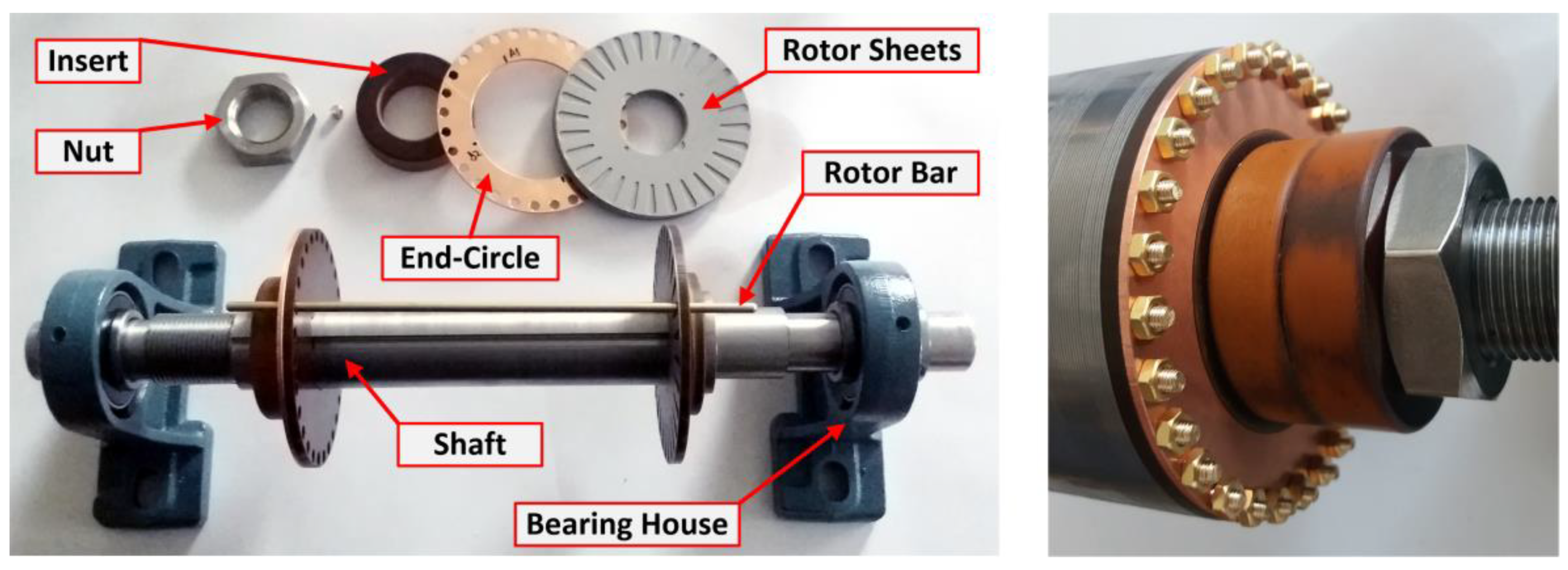
To verify the designed measurement technique and FEM simulations, a test rotor was manufactured. The test rotor consists of high grade non-oriented electrotechnical sheets type M530-65A with thickness th = 0.65 mm and total length of packet Lr = 150 mm. The sheet contains Ndr = 28 closed slots into which the brass rotor bars are inserted. The rotor sheets are not processed in any technological way before assembling into a packet and were randomly selected from the container of the cutting machine.

The rotor bars are made of brass with a diameter of d = 4 mm and are threaded at both ends. The end-rings are milled from copper sheet with a thickness of 2 mm. All rotor bars are insulated in the rotor slots by using insulating tubes. Similarly, the end-rings are separated from the rotor by an insulating plate and are not electrically connected to the rotor sheets. Figure 10 shows the individual parts of the rotor before it is assembled and partial view of the manufactured test rotor.

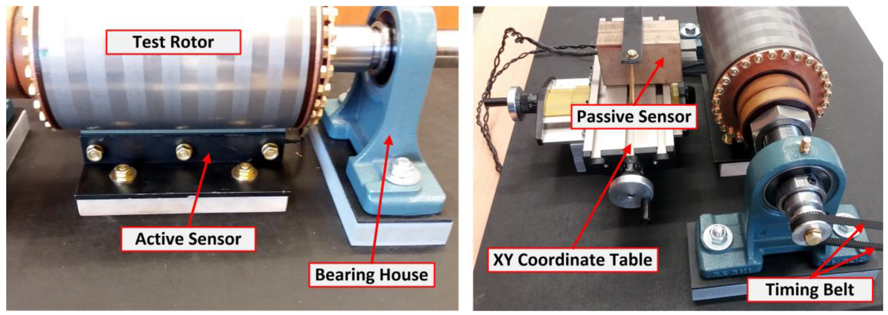
The rotor bars are fixed to the end-rings with nuts. The overall rotor arrangement was chosen to make fault simulation easier. The rotor allows testing, for example, a change in the conductivity of the end-ring, a break in the end-ring or part of the end-ring, a reduced conductivity of the bar, a broken rotor bar or a combination of these faults. A basic rotor measuring setup with sensor arrangement is shown in Figure 11.

The rotor rotation is ensured by the NEMA17 stepped motor operated by a driver via the Arduino module. The motor rotation speed is fixed to n = 180 rpm (3 rps), and it needs about 10 s to reach the set speed in linear acceleration mode. The stepped motor is attached to the rotor by timing pulleys and a rubber timing belt to eliminate the motor vibrations as well as to ensure exact revolution without slip. The shaft with the test rotor is placed in bearing housing.

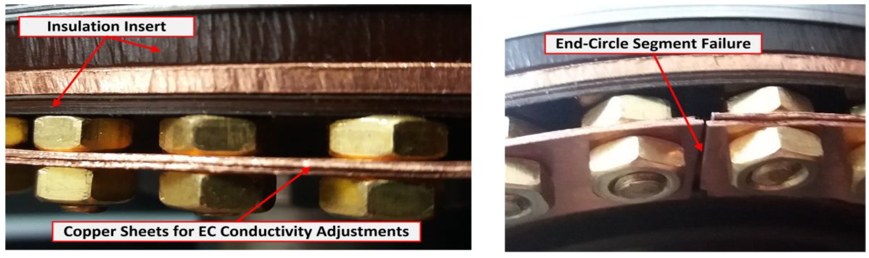
Figure 12 shows selected modifications to the test rotor end-ring to simulate its failure. Figure 12 shows the set-up for simulating the conductivity of the ring. Here, the original solid cross-section of the end-ring is replaced by a set of copper plates. The number of sheets determines the final value of the conductivity. Figure 12 also shows a simulation of a broken segment of the end-ring between the bars. The air gap causes a disconnection of the initially solid ring. The rotor bars remain conductively connected to the rest of the ring.

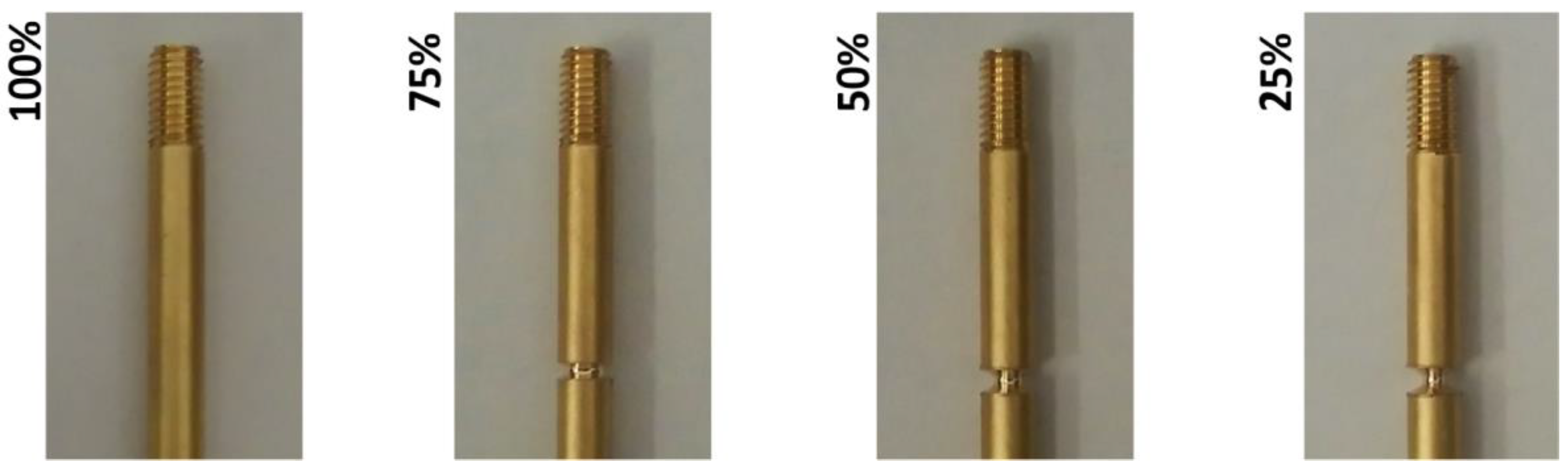
To simulate the defects of the rotor bars, geometric modifications were made to their cross-section as shown in Figure 13. Many of the authors [18,21,27] use direct drilling of rotor bars to create a defect. In our case, the reduction of the active cross-section of the bar is achieved by turning the cross-section at about 1/5 of its total length. The bars so prepared are sequentially inserted into the slot and the effect of the conductivity drop can be measured.

5. Processing of the Sensor Signals and Analysis

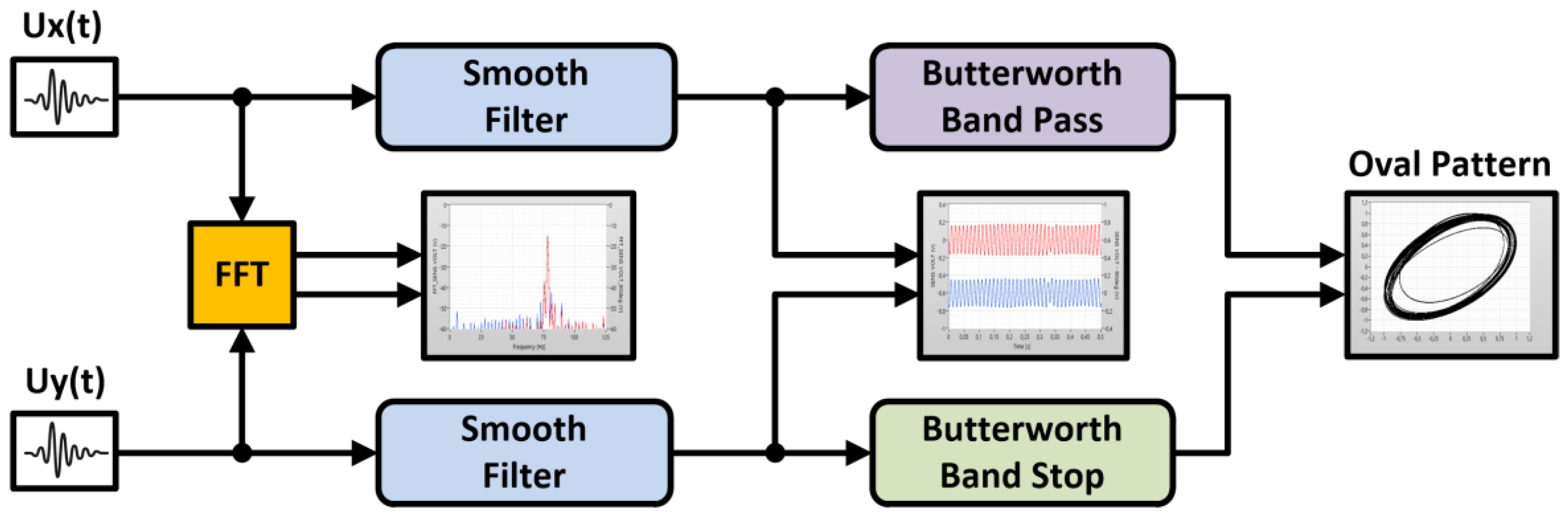
The measurement system is based on the LabView platform. The voltage outputs of both sensor signals are captured by the NI-DAQ card. FFT analysis is performed directly from the sensor signals. The signals are software smoothed and further amplified, filtered and processed, see Figure 14.

To find the type of rotor defect, the display of the FFT analysis results can be primarily used. However, for a regular operator without a higher qualification of signal analysis knowledge, the FFT analysis outputs can be very difficult to read. Some authors use signal shape comparison or evaluate a limit criterion for the appearance of sidebands in FFT analysis [30]. When evaluating a rotor defect, the operator often needs additional information, e.g., a view of the defect type. Therefore, we decided to use a technique known, e.g., in ovality or eccentricity measurements [34,35,36,37].

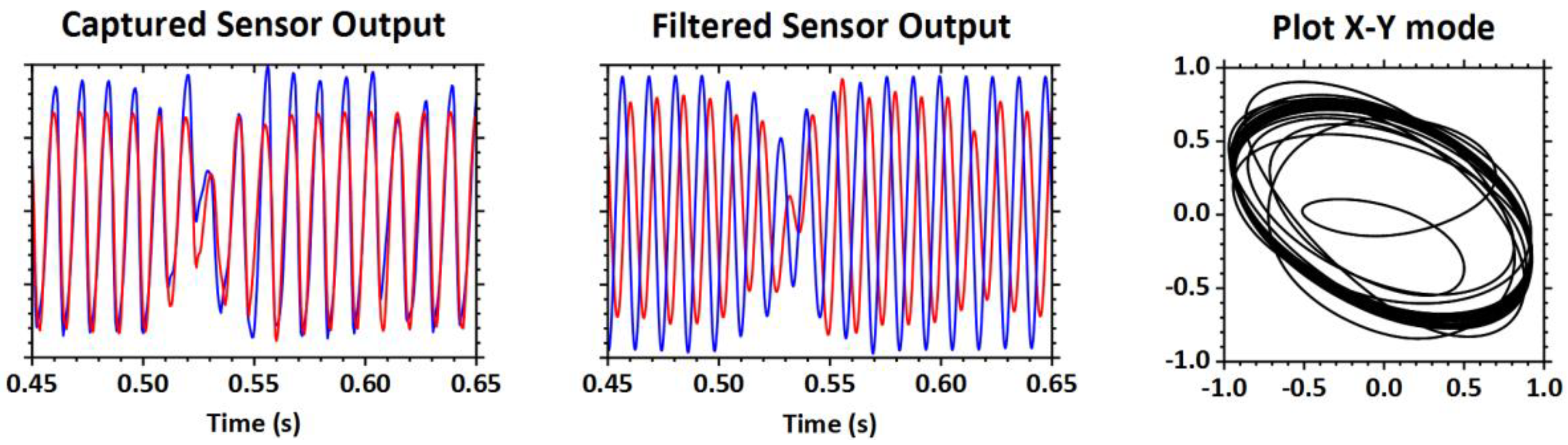
The basic principle is to display the signals from both sensors in X-Y mode. Both sensor signals have identical frequency fx = 84 Hz. The waveform of the signals is deformed and it is convenient to apply low-pass and high-pass filtering. The filters should be also set to highlight any deformation of the sensor signals. The rotor defect is reflected by the presence of sidebands in the region of the main harmonic—fx, as shown by FEM simulations, see Figure 8b and Figure 9b. Thus, we apply the filtering of the signals close to the frequency of the main harmonic fx = 84 Hz. A filter setting with the following parameters was found to be the most effective, see

Table 1. Basic types of active filters and their configuration settings.

Type of Filter	Order (-)	Freq Low (Hz)	Freq High (Hz)
Butterworth Band Pass	4th	fx/2 (42)	3 × fx/2 (126)
Butterworth Band Stop	4th	fx + 1 (85)	Higher than 10 × fx (1000)

.

Butterworth Band Pass and Butterworth Band Stop filtering adds a phase shift naturally to both signals [38,39]. We use this mutual phase shift of the two signals in the X-Y mode display, which is then represented by an oval shape, see Figure 15.

Using the X-Y mode display, we can evaluate the quality of the rotor based on the change in the specific shape of the oval. With a test rotor, we can attempt to find these basic shapes.

Measurement Outputs—Displaying and Comparison of Oval Patterns

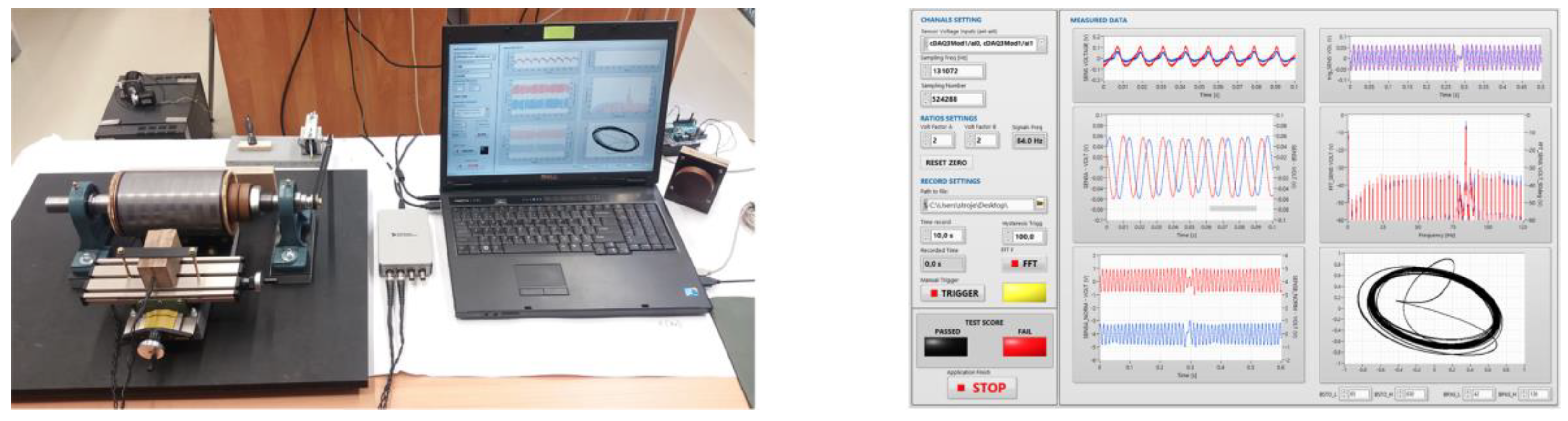
The basic arrangement of measurements on the test rotor is shown in Figure 16. On the left is the base with test rotor and sensors, on the right is the PC with LabView and visualization panel.

Figure 17 shows the measured voltage time waveforms from both sensors and the FFT spectrum of the signals when the rotor is simulated without defects. The assembled test rotor shows eccentricity, which is clearly visible in the waveforms. The eccentricity is caused by assembling the rotor sheets on the shaft without additional machining. The voltage waveform is uniform with no distortion or deformation.

The eccentricity is indicated by a slight movement of the envelope. In the FFT analysis, increased sidebands appear around the dominant harmonic fx = 84 Hz. The passive sensor has a better response to eccentricity, which is reflected in the FFT analysis by the presence of a sideband even at lower frequencies with a maximum amplitude of −38 dB.

Figure 18 shows the waveforms for the broken bar simulation. The voltage waveforms of the two sensors captured in the interval t = (0.5 ÷ 1.0) s show periodically repeating distortions, which indicate the missing part of the induced voltage. In FFT analysis, significant sidebands are formed on both sides of the dominant harmonic fx = 84 Hz. The signal to maximum amplitude offset is about −26 dB.

In the simulation of a broken end-ring segment, see Figure 19, the waveform of the induced voltages deforms differently. The voltage waveform at the defect location shows only a slight drop at the active sensor, while the passive sensor responds to the missing end-ring segment with a significant voltage jump in the voltage waveform. The sidebands in this fault form more in the lower frequencies, the higher frequencies gradually decay with harmonic order. The passive sensor shows a better sensitivity to this type of fault and the level of signal offset here is about −32 dB, the active sensor shows a lower level, about −42 dB.

With the sensor voltage waveforms and their FFT analysis, the X-Y mode patterns are plotted to provide additional information for easier rotor fault identification. To verify the functionality of the pattern plotting, the basic types and ranges of defects that can occur during rotor casting were determined. Overall, the defined groups of simulated test rotor defects are presented in

Table 2. Subdivision of rotor failures simulated on testing rotor.

Rotor Defect	Description	Identification Case
No Defects	Healthy Rotor	000
Bar Conductivity	25% Cross-Section Loss	A
(Porosity)	50% Cross-Section Loss	B
	75% Cross-Section Loss	C
Bars	1 Broken Bar	D
(Broken Bars)	2 Broken Bars	E
	3 Broken Bars	F
End-Ring Segment	33% Cross-Section Loss	G
(Porosity)	67% Cross-Section Loss	H
	100% Cross-Section Loss	I
Combined Rotor Failures	1 bar + 1ER Segment	J
	1 bar + 2ER Segment	K
	2 bars + 1ER Segment	L

.

The rotor defects were divided into 4 groups. The first group of defects relates to internal defects in the bars where impurities or material porosity may be present. The second group of defects simulates completely cracked rotor bars that remain part of the rotor but are electrically disconnected from the end-rings. The third group simulates an end-ring defect due to porosity in a selected segment of the ring between two bars. The last fourth group describes a combination of faults caused by the combination of an end-ring and rotor bar fault. The simulated rotor defects are incrementally increased to capture the change in plotting and deformation of the displayed patterns.

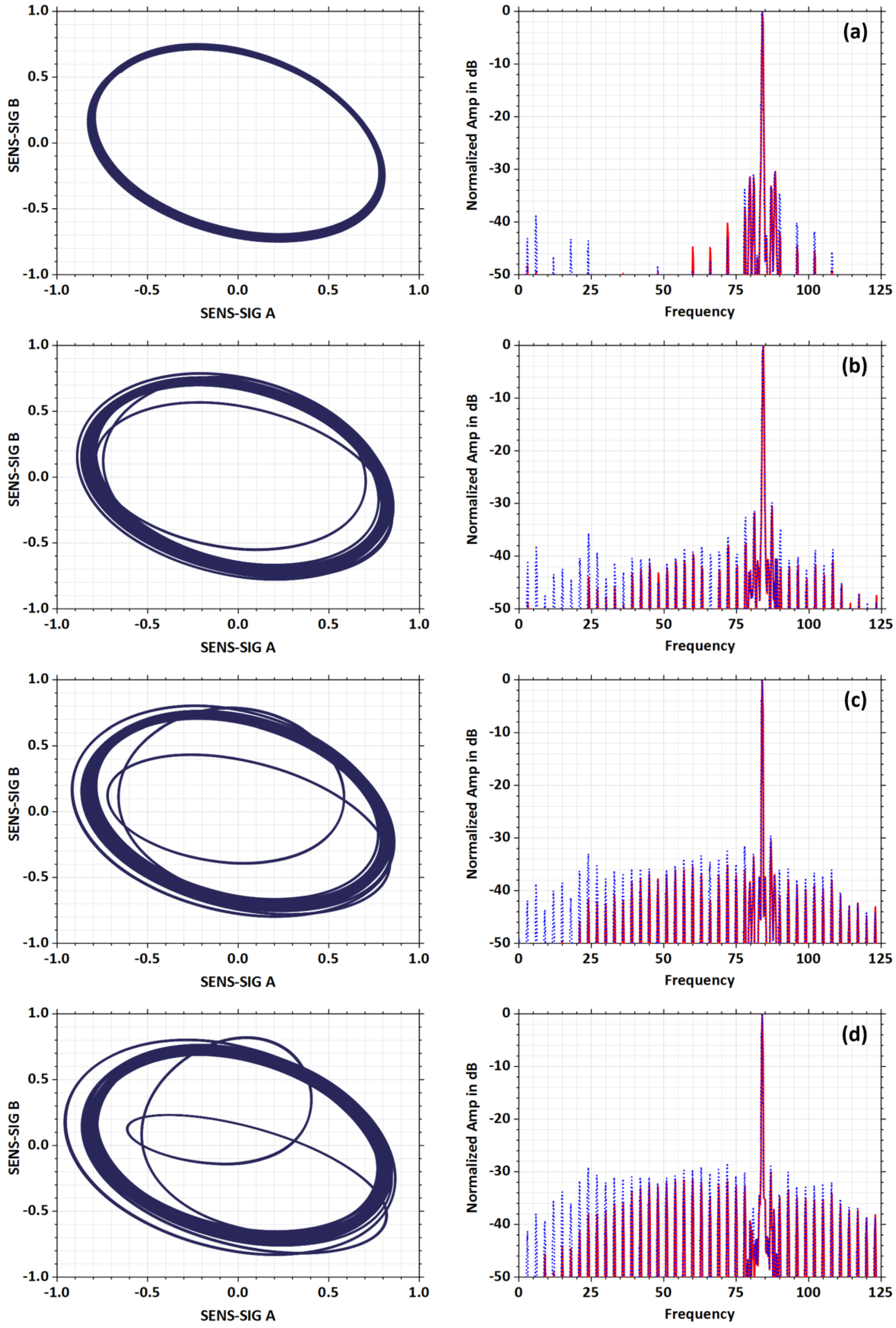
Figure 20 shows the dependencies as the electrical conductivity of the 1 pc rotor bar is incrementally reduced. At the same time, the effect of the decreasing cross-section of the rotor bar on the spectrum of FFT analysis and the plotting of oval patterns is also compared. The orbiting point at the boundary of the oval traces the voltage dependence between the two sensors. In one revolution of the test rotor, the pattern contains 28 orbits of the plotting point. Ideally, in a rotor without defects, the pattern takes the form of a smooth oval whose thickness is affected by the eccentricity, see Figure 20a.

As the bar resistance increases, the plotting point gradually separates, see Figure 20b–d, as the voltage waveforms respond by decreasing the induced voltage at the defect bar location. At a 25% loss in bar conductivity, a deflection from the original defect-free oval becomes apparent. At 75% bar conductivity loss, the plotting point circulates near the center of the oval. The rotor failure is easily identified even with a relatively small drop in bar conductivity.

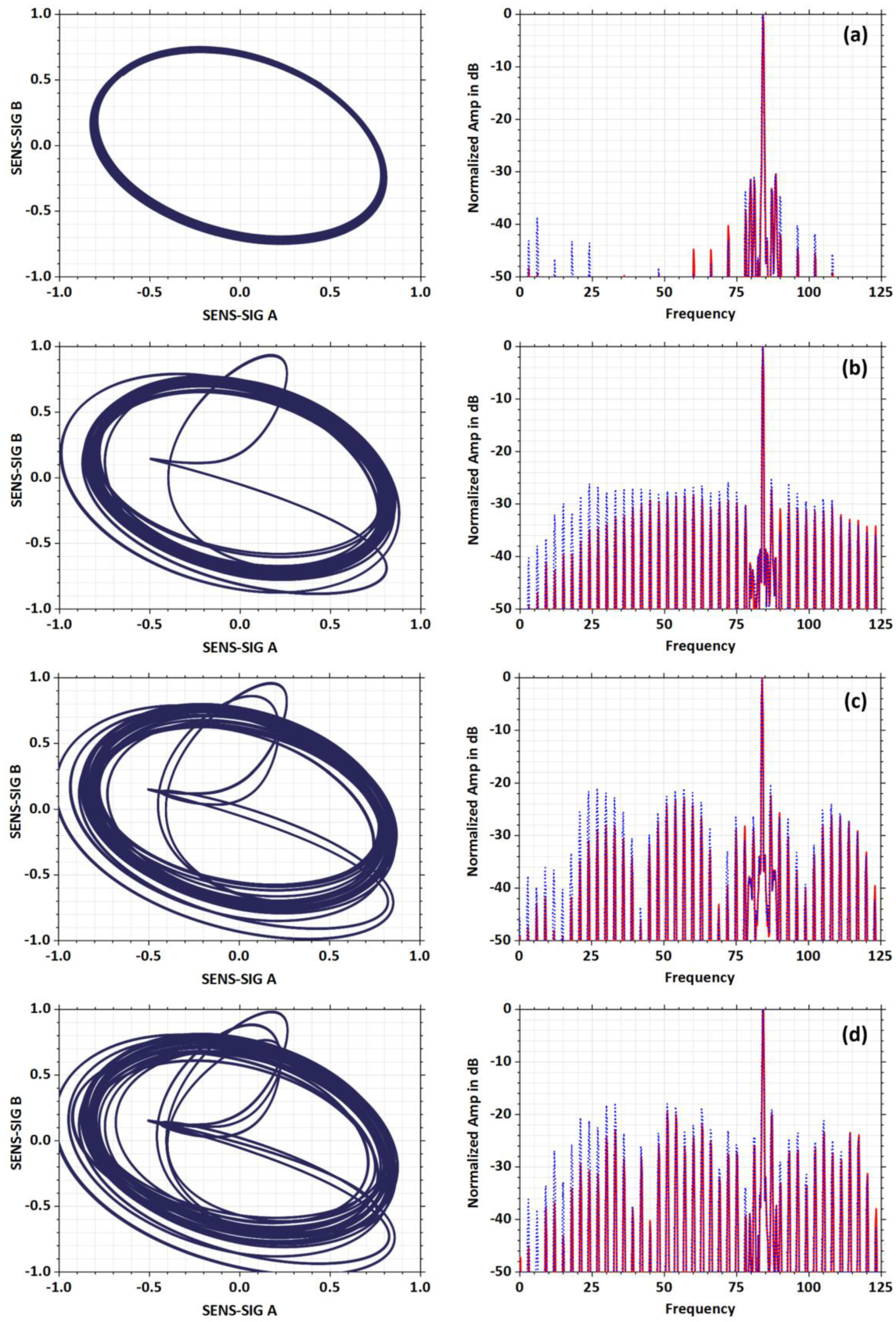
Figure 21 shows the deformation of the oval pattern when the rotor bars are completely broken. The number of broken bars is gradually varied during the test. The 1 pc of a completely broken bar plots a multiple curve on the oval with a characteristic sharp point in the center of the oval, see Figure 21b. If the number of broken bars is higher, the number of these crossed curves increases. Furthermore, there is also separation of the oval on its lateral sides, see Figure 21c,d. The shape of the crossed curves depends on the relative position of the broken bars in the rotor, but they always pass through the center of the oval.

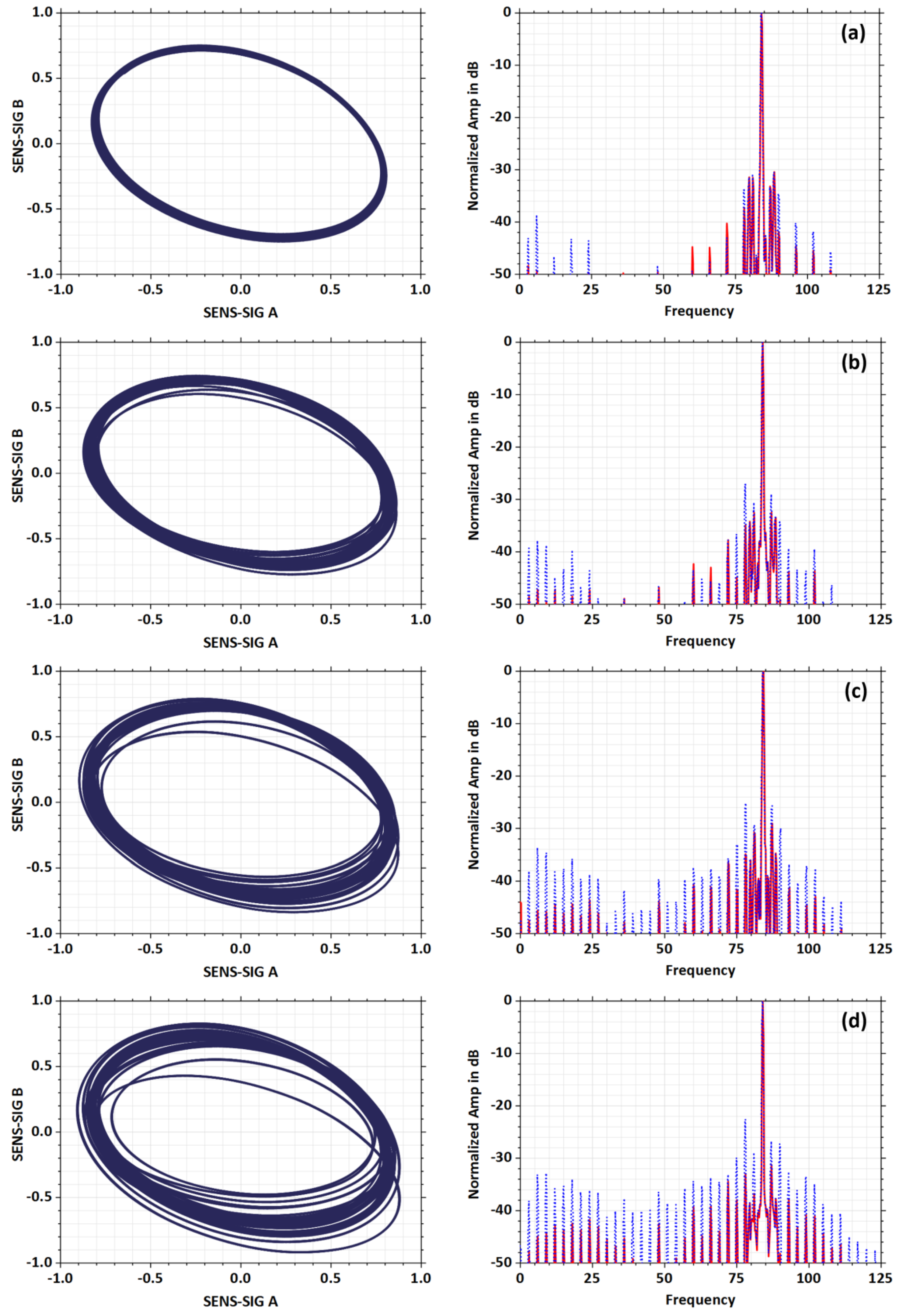
Figure 22 shows the change in the overall deformation of the oval pattern when a failure occurs in a segment of the end-ring. The change in the conductivity of the connection between the two bars of the initially separated segment was simulated. As the conductivity of the segment decreases, the proportions of the oval remain almost identical, but its inclination in the symmetry longitudinal axis changes significantly. With a fully broken segment between the bars, see Figure 22d, the plotting point moves along a set of elliptic curves that are rotated relative to each other. The measurement sensitivity is lower in this case, which is also evident from the FFT analysis of the spectra. This fault is better visible in the passive sensor, which shows a faster increase in sideband amplitudes.

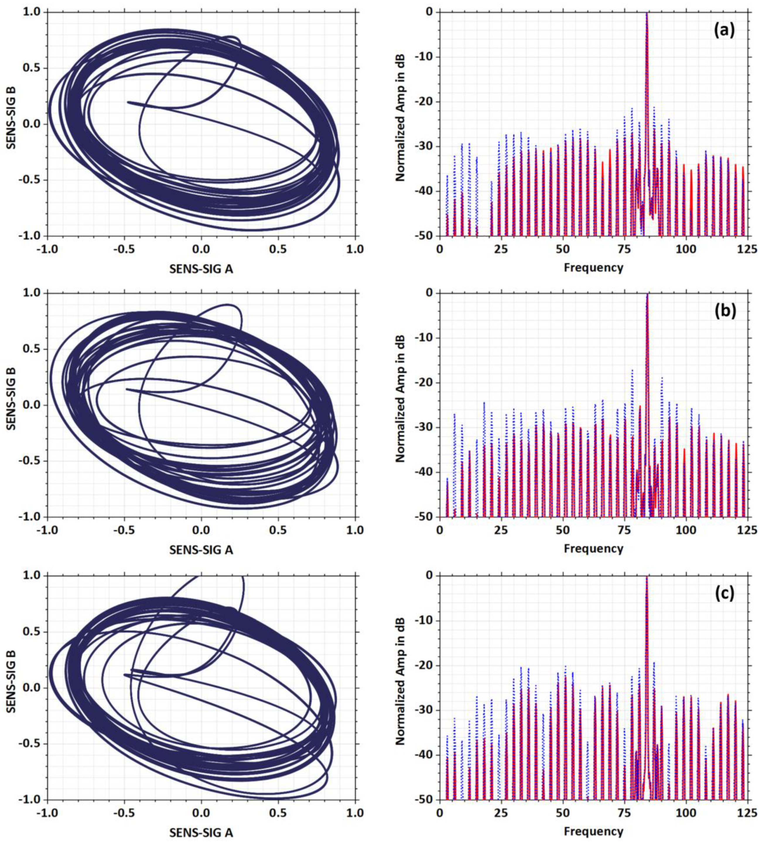
Combined rotor failures are shown in Figure 23. A broken bar in combination with a broken segment of the end-ring or multiple failures such as 2 broken bars with a broken segment, etc., cause significant deformation of the originally smooth oval pattern. The plotting point gradually separates from the original oval pattern in multiple sequential steps. The patterns also tilt and form internal loops. Their final form is in fact a composite of the patterns typical of the elementary faults in Figure 21 and Figure 22. The sidebands in the FFT analysis completely fill the space to the left and right of the dominant harmonic fx = 84 Hz and illustrate the significance of the fault simulated on the test rotor.

6. Off-Line Measurement of Real Squirrel Cage Rotors after Casting Process

The designed measurement procedure and sensor configuration was verified on several real rotor prototypes. Figure 24 shows the basic arrangement of the measurement system with the rotor fixed between the aluminum conical centering tips. Figure 24 also shows representative rotor samples prepared for defect detection. The rotor samples are unmachined, without shafts, and were collected after casting and cooling.

Measurements were in general the same as in the previous test rotor. However, the main task was different and was to use the visualized oval pattern to determine the fault in the end-ring or rotor bars. Most of the tested rotors represented by sample R1 displayed a pattern similar to that shown in Figure 25. The oval shape is relatively smooth, its thickness being affected by eccentricity. FFT analysis indicates only a thin sideband concentrated around the dominant harmonic fx = 84 Hz. The measured prototype rotors contain Ndr = 20 fully closed slots, and the rpm had to be set higher than the test rotor. The frequency band offset thus reaches Δf = 4.2 Hz.

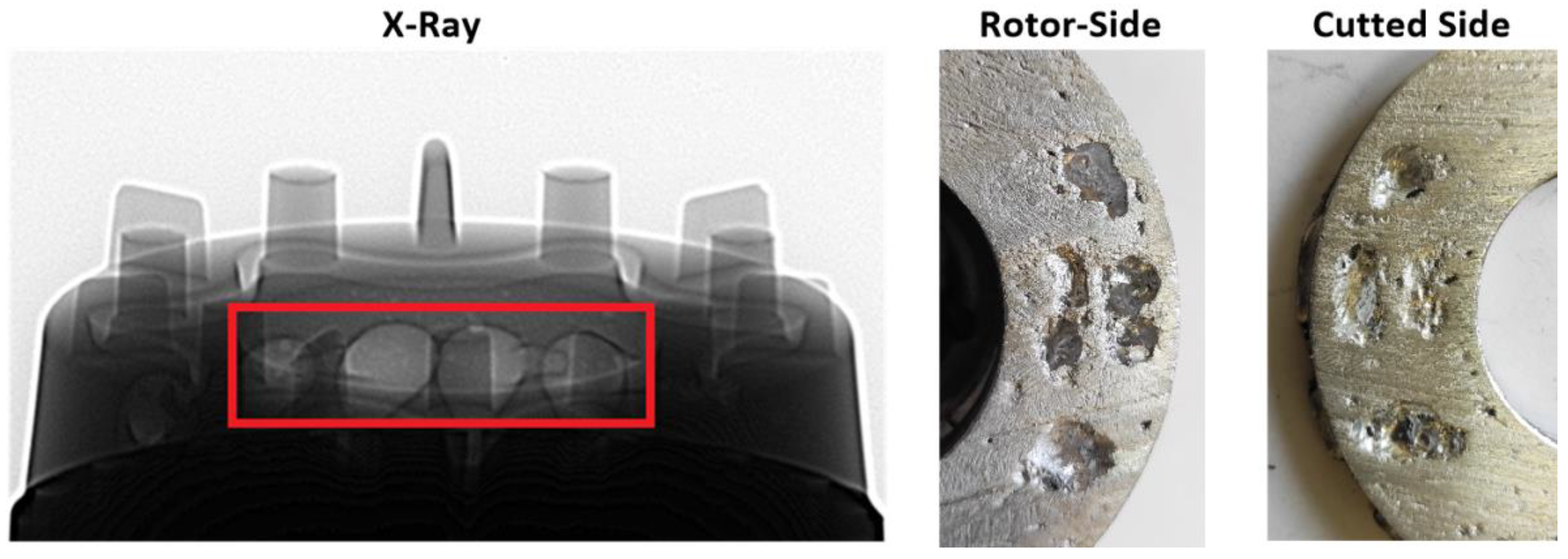
In the group of rotors, a sample labeled R2 was found that showed a different oval shape, see Figure 26. FFT analysis indicated the appearance of a sideband in the lower frequency range. The oval pattern is separated and the plotting point circulates along mutually tilted elliptical shapes. From this output, we assumed that this is a fault in the end-ring.

The assumption was finally confirmed by two methods, see Figure 27. X-ray photography shows the presence of air bubbles that almost completely fill the volume of the end-ring. The destructive method of cutting through the end-ring illustrated the scale of this defect, which significantly reduces the conductivity of the end-ring segments.

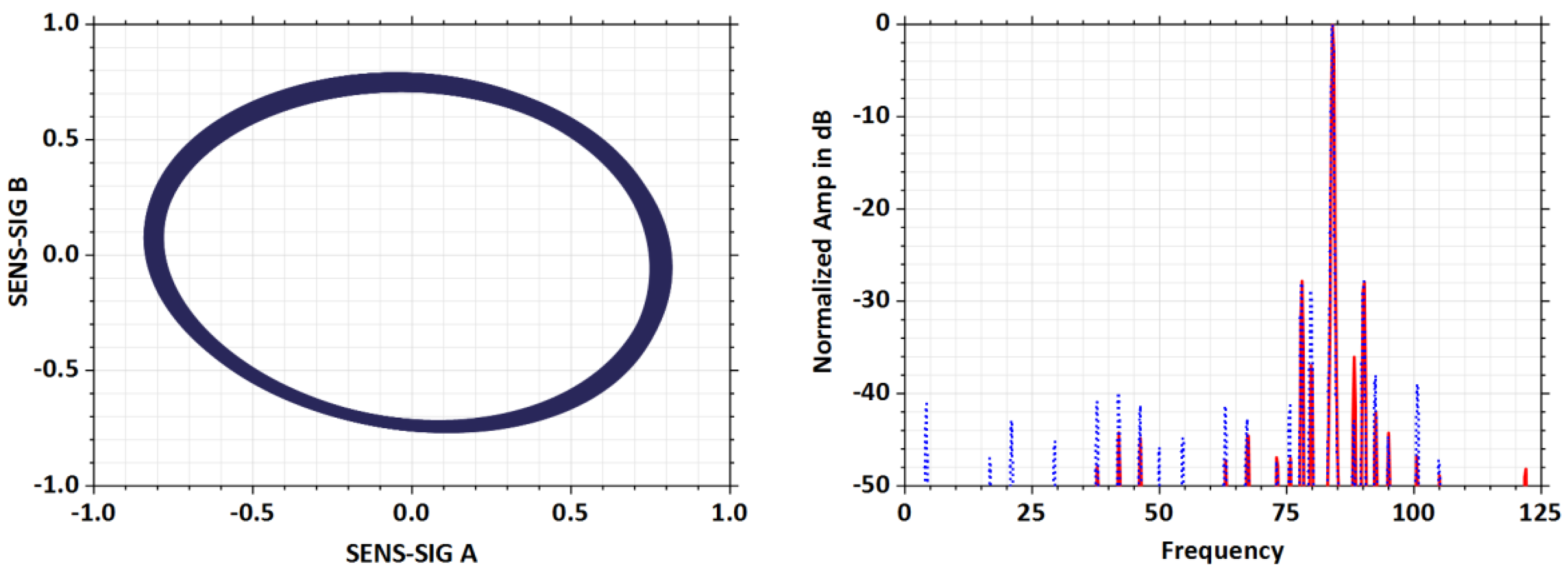
The rotor labeled R3 presents a sample with a combined fault in the rotor bars, see Figure 28. The internal crossing of the trajectory of the plotting point is characteristic of a fault in the rotor bars.

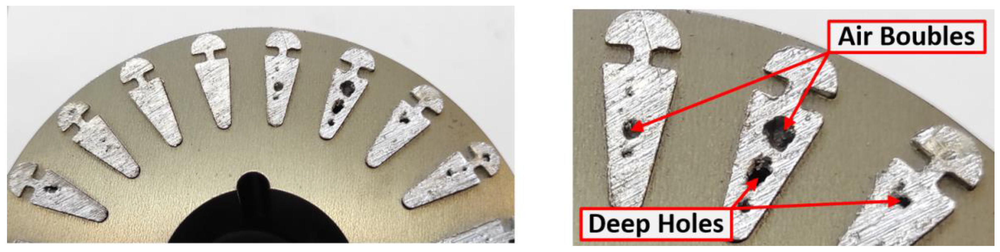
The FFT analysis indicates a significant presence of sidebands on both sides of the dominant harmonic and also a better sensitivity of the passive sensor to this type of fault. A cut made at 1/3 of the rotor length exposed air bubbles and deeper holes in several rotor bars, see Figure 29.

However, this does not automatically imply that the presence of failures in this cross-section is complete. According to the oval pattern, there are probably more damaged bars, or bars with a high content of air bubbles or holes, in the tested rotor R3.

7. Discussion

The proposed system of fault detection by using a graphical pattern is based on the principle of voltage induction in a conductor (bar) moving in a static magnetic field. The 2-sensors measurements were used to determine the quality of the manufactured rotor. The overall summary of the advantages and disadvantages of the methodology used is organized in the following sections:

(A)

Sensor design

The magnetic field is generated by permanent magnets in the active sensor enclosure. The advantage of this solution is the absence of excitation current, which is otherwise necessary when using a classical growler yoke. To sufficiently magnetize the rotor teeth, rather strong NdFeB magnets are needed. The excitation cannot be adjusted, therefore the air gap between the excitation yoke and the rotor surface must be relatively small. This makes the excitation sensitive to sticking of ferromagnetic particles and sawdust. In laboratory conditions this is not a problem in principle, but if the measuring system is implemented in a production cycle, it must be remembered that sawdust can eventually create a magnetic short circuit between the poles of the active sensor.

(B)

Test system assembly

It is important to keep in mind the influence of the surrounding environment. The ferromagnetic mass enclosing the rotor to be measured can cause high distortion in the sensed signals. In our case, the massive clamping head showed to be the biggest problem. The clamping system has to be made with non-magnetic rods that are far enough away from the actual rotor body.

(C)

Calibration of sensors using a test rotor

The adjustment and validation of the methodology used was verified on a test rotor. The design of the test rotor should be as close as possible to the real rotor. This was not fully met in our case. The real squirrel cage rotor does not contain isolated rotor bars as in the case of the test rotor. During die casting, the rotor slots are filled with molten aluminum and the rotor bar comes into direct contact with the rotor plates. There is a high probability of interbar currents, where the electric current flows partially through the rotor plates and can bypass a minor defect inside the bar. The cross-section of the bar in a real rotor is not circular. The real rotor contains a double cage, see Figure 29. In addition, the thickness of the end-ring of the real rotor is large, see Figure 24. If the air bubbles occupy a significant part of the end-ring cross-section, then this defect is quite detectable. However, if the porosity of the air bubbles is smaller, the proposed measurement system shows lower sensitivity.

(D)

Criteria for evaluating patterns, sensitivity

For a real rotor without defects, the trajectory of the plotting point in X-Y mode forms a regular and smooth oval. The shape and dimensional proportions of this oval are identical for identical rotors without defects. Such a rotor then plots a trajectory in X-Y mode which is the reference for other measured rotors of identical design. The outer and inner border of the oval is defined by the trajectory of the plotting point, which runs in a specific range around its perimeter. This produces the typical width of the oval, the magnitude of which is determined by the eccentricity for a rotor without defects. The eccentricity can be adjusted by using clamping conical tips inserted into the shaft bore and verified on the induced voltage time histories included in the test window.

Fault identification is based on graphical and visual comparison of the plotted pattern with a reference oval shape. The visual assessment is (i) the increase in the width of the oval from the reference pattern, (ii) the separation of the trajectory of the plotting point from the reference width of the oval, (iii) the tendency of the plotting point to form internal loops inside the oval, (iv) the number of internal loops formed.

In the case of a minor defect in the rotor bar, the deformation of the plotting point trajectory may not be completely evident for an accurate specification of the type of failure. By looking at the FFT analysis window, which is also part of the test panel, the rotor fault can be specified more precisely. A double-sided sideband indicates a fault in the bar, a left-sided sideband represents a fault in the ring. Unfortunately, the sensitivity to defects in the end-ring is less for the fabricated test system than for defects in the bars.

(E)

Measurement outputs from test and real rotors

As can be seen from Figure 20b, a defect in the rod (air bubble, reduced conductivity) is only detectable at approximately 25% loss in rod cross-section. It was observed that at lower fault ranges <25% of rod cross-section loss, the pattern only slightly expands and the fault resolution is worse. The fault is much more identifiable on FFT analysis of both signals. In the case of a completely cracked bar or set of bars, the patterns on Figure 21b–d show a significant deviation of the plotting point from the original oval shape and these types of faults are very well identifiable. In the second phase of verification, the defects in the end-ring were measured. Again, it is evident that the range of damage (porosity) had to achieve at least 30% cross section loss for this defect to be reasonably visible, see Figure 22b.

Comparing the bar and end-ring defect, the difference in the trajectory of the plotting point is evident. With the bar fault, the thickness of the oval only slightly expands, and the trajectory of the plotting point forms an internal crossing. The oval gradually separates in the upper left part. In an end-ring fault, the individual ovals are separated and slightly rotated. The effect of the segment porosity is reflected by the trajectory deviation in the lower part of the oval. The passive sensor is located approximately in the middle of the rotor length during the measurement, and thus actually captures an image of the instantaneous value of the current in the bar determined by the fault condition in the end-ring segment. The detectability of a fault in the end-ring can be improved if the passive sensor is located closer to the end-ring and oriented parallel to the axis of rotation of the rotor being measured.

For a real rotor without defects, the trajectory of the rendering point in X-Y mode forms a regular and smooth oval, see Figure 25. The defect in the real rotor can no longer be explicitly set, as in the case of the test rotor, but the fault identification is performed directly. As can be seen from Figure 26 and Figure 28, the defects in the real rotor are more likely to occur in a combined form. The oval in Figure 26 tends to increase in thickness and there is only a slight crossing of the plotting point trajectory. The frequency band is centered to the left of the dominant harmonic fx = 84 Hz. The shape of the oval shows a character consistent with an end-ring defect. A series of crossings and inner loops appear in Figure 28. The loops in the center of the oval are smooth and do not contain sharp shapes. The bars in the rotor will not be completely interrupted, but considerable porosity can be expected. One of the rods has a very significantly reduced conductivity. The frequency band appears on either side of the dominant harmonic fx = 84 Hz.

8. Conclusions

The paper dealt with off-line diagnostics of the rotor of an asynchronous machine using two sensors. The functionality of the whole system for measuring and identifying faults in the rotor was firstly verified using a 2D FEM electromagnetic model. The FEM analysis was also used to find the appropriate arrangement of the sensors and their optimal position near the rotor. To validate the measurement system, a test rotor was built to simulate the specific types of faults and their possible combinations that can occur in squirrel cage rotors. The evaluation system includes a graphical fault visualization interface that displays voltage waveforms, FFT signal analysis, and oval patterns and is used to identify specific rotor faults. It was important to find characteristic pattern shapes whose shape corresponds to the simulated fault. The graphical outputs of the patterns serve as additional information for the operator to evaluate the quality of the manufactured rotor. If the plot point deviates significantly from the reference shape of the regular oval, the rotor can be considered as defective and can be removed from the next production process. The final decision can be made by the operator or by the automated system.