Two-Phase Flow Effects on Seismic Wave Anelasticity in Anisotropic Poroelastic Media

Abstract

We study the wave anelasticity (attenuation and velocity dispersion) of a periodic set of three flat porous layers saturated by two immiscible fluids. The fluids are very dissimilar in properties, namely gas, oil, and water, and, at most, three layers are required to study the problem from a general point of view. The sequence behaves as viscoelastic and transversely isotropic (VTI) at wavelengths much longer than the spatial period. Wave propagation causes fluid flow and slow P modes, inducing anelasticity. The fluids are characterized by capillary forces and relative permeabilities, which allow for the existence of two slow modes and the presence of dissipation, respectively. The methodology to study the physics is based on a finite-element uspcaling approach to compute the complex and frequency-dependent stiffnesses of the effective VTI medium. The results of the experiments indicate that there is higher dissipation and anisotropy compared to the widely used model based on an effective fluid that ignores the effects of surface tension (capillarity) and viscous flow interference between the two fluid phases.

1. Introduction

Wave anelasticity in porous media is a topic with applications in many areas of geophysics and material science [1]. Waves generate fluid flow in the pores and energy losses that can be observed in field and laboratory experiments [2,3,4]. Recent laboratory experiments performed in the seismic range have shown the frequency dependence of anelasticity in sandstones with partial gas or oil saturations [5,6,7], while experiments conducted in Reference [8] show a significant attenuation in the extensional and bulk deformation modes, as well as numerical simulations in close agreement with laboratory data.

The theoretical pioneering work of Biot [9,10,11] describes waves propagation in porous media saturated by single-phase fluids. The theory predicts a shear wave and two compressional waves, a fast one, where the solid and fluid move together, and a slow one, where the displacement is out of phase. At low frequencies, the slow wave is diffusive and becomes a propagating wave at high frequencies. Significant anelasticity of the fast wave is due to mode conversion at mesoscopic scale heterogeneities (mesoscopic loss). White et al. [12] were the first to introduce this loss mechanism based on Biot’s theory for a periodic sequence of two flat and thin porous layers saturated with a single-phase fluid. This mechanism is also termed WIFF or wave-induced fluid flow loss.

The study of propagation in partially saturated porous media has been presented in References [13,14,15]. Lo et al. [16] present an Eulerian model for waves propagating in porous media saturated by two fluids. In this model, the stress-strain relations are obtained by taking into account capillary pressure assumed as a unique function of saturation and ignoring hysteresis, while the dynamic equations are formulated from a mass balance equation for each solid and fluid phase. Three compressional waves are predicted to exist, one wavelike and two of them of diffusive type. The model is applied to analyze waves in soils saturated by water with air or oil. A macroscopic model based on a two-component Biot model and a mixture theory is presented in Reference [17]. Other models to analyze the wave behavior in porous rocks saturated my immiscible fluids appeared in [1,15,18,19,20,21,22]

Concerning studies on porous media by using numerical simulations, the work by Thovert et al. [23] analyzes wave propagation using an homogenization approach. The authors consider the existence of connected pores that may or may not percolate, obtain the macroscopic coefficients and apply the results to a synthetic porous medium. Hamzehpour et al. [24] study acoustic waves in two-dimensional fractured porous media using finite differences to discretize the differential equations. This analysis concludes that, near the source, waves amplitude decay exponentially. A generalization of the Biot theory, appearing in Reference [25], takes into account more than one fluid phase saturating the pores, such as brine-gas and oil-gas mixtures. This theory predicts three compressional waves and a shear wave. The stress-strain relations are derived from the complementary virtual work principle in order to include the capillary pressure relation, while the dissipation function is defined in terms of Darcy’s law based on two fluids [26].

The presence of an additional slow wave is expected to induce more attenuation and velocity dispersion, as shown in Reference [27], for the case of vertical propagation across a periodic set of two thin layers saturated with two immiscible fluids. This work considers the more general case of a sequence of three layers, also leading to a VTI behavior at long wavelengths, but to a different frequency dependence of the velocity and attenuation. Qi et al. [28] consider capillary effects in random media of patchy saturation by using a membrane stiffness, but this approach leads to an increase in phase velocities and lower attenuation. An experimental study on how capillarity affects the compressional P-wave velocity for patchy saturation during an imbibition process is presented by Liu et al. [29], where the patch size depends on the fluid saturation. The effect of capillarity is related to the injection rate, changing with imbibition. The results exhibit an increase of the experimentally measured P-wave static velocity as capillary pressure increases.

This study is based on the theory of Cavallini et al. [30] valid for periodic N layers saturated for single-phase fluids and a FE procedure to obtain an equivalent VTI medium to an horizontally layered medium consisting of a three periodic poroelastic solid saturated by immiscible fluids. An FE procedure is used to determine a VTI medium equivalent at long wavelengths to a periodic sequence of thin poroelastic layers. It consists of defining five independent boundary-value problems, each one associated with either a compressibility or shear time-harmonic test, whose solutions are obtained by the FE method. The results are validated against the theory by Cavallini et al. [30] for effective single-phase fluids. Then, several examples are given, where the velocities and attenuation are obtained by using effective-single phase and two-phase fluids.

2. The Differential Model

The poroelastic medium is saturated by non-wetting and wetting fluid phases, whose properties and variables are indicated by subscripts or superscripts “n” and “w”, respectively. The corresponding saturations are denoted by $S_w=S_w\left(\mathbf{x}\right)$ and $S_n=S_n\left(\mathbf{x}\right)$, with $\mathbf{x}=(x,y,z)$, respectively, with associated residual saturations $S_{rw}$ and $S_{rn}$. It is assumed that both fluid phases occupy the whole pore space and that a continuous network of these phases exists (funicular regime) [31]. Thus,

$$S_w+S_n=1,S_{rn}<S_n<1-S_{rw},S_{rw}<S_w<1-S_{ro}.$$

The Fourier transforms of the particle displacement of the three phases composing the material, i.e., the solid, non-wettting and phases phases, are denoted as ${\mathbf{u}}^s=\left(u_i^s\right)$, ${\tilde{\mathbf{u}}}^n=\left({\tilde{u}}_i^n\right)$, and ${\tilde{\mathbf{u}}}^w=\left({\tilde{u}}_i^w\right),i=1,2,3$, respectively. Set $\mathbf{u}=({\mathbf{u}}^s,{\mathbf{u}}^n,{\mathbf{u}}^w)$. Define $\varphi =\varphi \left(\mathbf{x}\right)$ as the matrix effective porosity, with the relative displacement and variation in fluid content of each fluid phase defined as

$${\mathbf{u}}^{\theta }=\varphi ({\tilde{\mathbf{u}}}^{\theta }-{\mathbf{u}}^s),{\xi }^{\theta }=-\nabla ·{\mathbf{u}}^{\theta },\theta =n,w.$$

Define $P_w$ and $P_n$ as the Fourier transforms of infinitesimal changes in the wetting and non-wetting fluid pressures, respectively, with respect to an initial equilibrium state of pressures ${\overline{P}}_w$, ${\overline{P}}_n$, porosity $\overline{\varphi }$, and non-wetting saturation ${\overline{S}}_n$. The capillary relation is [26,31,32]

$$\begin{array}{c}\hfill P_{ca}=P_{ca}(S_n+{\overline{S}}_n)={\overline{P}}_n+P_n-({\overline{P}}_w+P_w)=P_{ca}\left({\overline{S}}_n\right)+P_n-P_w\ge 0.\end{array}$$

(1)

Ignoring hysteresis, $P_{ca}$ is an increasing function of $S_n$ and positive.

Let ${\epsilon }_{ij}\left({\mathbf{u}}^s\right)$ and $e^s={\epsilon }_{ii}\left({\mathbf{u}}^s\right)$ be the Fourier transforms of the solid strain tensor and corresponding linear invariant, respectively. Denoting with ${\tau }_{ij}\left(\mathbf{u}\right)$ the stress-tensor components of the bulk material, the constitutive relations are:

$$\begin{array}{ccc}& {\tau }_{ij}\left(\mathbf{u}\right)\hfill & =2\mu {\epsilon }_{ij}+{\delta }_{ij}({\lambda }_u{e}^s-B_1{\xi }^n-B_2{\xi }^w),\hfill \end{array}$$

(2)

$$\begin{array}{ccc}& {\mathcal{T}}_n\left(\mathbf{u}\right)\hfill & =\left({\overline{S}}_n+\beta \right)P_n-\beta P_w=-B_1{e}^s+M_1{\xi }^n+M_3{\xi }^w,\hfill \end{array}$$

(3)

$$\begin{array}{ccc}& {\mathcal{T}}_w\left(\mathbf{u}\right)\hfill & ={\overline{S}}_w{P}_w=-B_2{e}^s+M_3{\xi }^n+M_2{\xi }^w,\hfill \end{array}$$

(4)

where

$$\beta ={\displaystyle \frac{P_{ca}\left({\overline{S}}_n\right)}{P_{ca}^{\prime }\left({\overline{S}}_n\right)}}.$$

In (2), ${\lambda }_u=K_u-\frac{2}{3}\mu$, with $K_u$ and $\mu$ being the wet-rock bulk and dry-rock shear moduli, respectively. Thus,

$$\begin{array}{c}\hfill E_u={\lambda }_u+2\mu \end{array}$$

(5)

is the wet-rock P-wave modulus. The coefficients in (2)–(4) can be determined as indicated in Appendix A.

The model describing the response of a poroelastic medium saturated with two fluids in the diffusive range of frequencies consists of a partial differential equations imposing the stress equilibrium of the bulk material (Equation (6)), together with a generalization of the two-phase Darcy law [26,31,32] (Equations (7) and (8)). Thus, if $\omega$ denotes the angular frequency, these equations are

$$\begin{array}{ccc}& & \nabla ·\tau \left(\mathbf{u}\right)=0,\hfill \end{array}$$

(6)

$$\begin{array}{ccc}& & i\omega d_n{\mathbf{u}}^n-i\omega d_{nw}{\mathbf{u}}^w+\nabla {\mathcal{T}}_n\left(\mathbf{u}\right)=0,\hfill \end{array}$$

(7)

$$\begin{array}{ccc}& & i\omega d_w{\mathbf{u}}^w-i\omega d_{nw}{\mathbf{u}}^n+\nabla {\mathcal{T}}_w\left(\mathbf{u}\right)=0.\hfill \end{array}$$

(8)

The coefficients in (7) and (8) depend on the absolute permeability $\kappa$, fluid viscosities ${\eta }_l$ and relative permeabilities $K_{rl}\left(S_l\right)$, $l=n,w$. They are defined as

$$\begin{array}{ccc}& & d_l\left({\overline{S}}_l\right)={\left({\overline{S}}_l\right)}^2{\displaystyle \frac{{\eta }_l}{\kappa K_{rl}\left({\overline{S}}_l\right)}},l=n,w,\hfill \end{array}$$

(9)

$$\begin{array}{ccc}& & d_{nw}({\overline{S}}_n,{\overline{S}}_w)=ϵ\left(d_n\left({\overline{S}}_n\right)d_w\left({\overline{S}}_w\right)\right).\hfill \end{array}$$

(10)

The coefficient $d_{nw}\left(S_n\right)$ in (10) is a dissipative function, where $ϵ$ is small. It describes the viscous drag between the immiscible fluids. In the absence of experimental data, it has the form given in (10).

3. The Equivalent Viscoelastic Transversely-Isotropic Medium

For long wavelengths, compared to the layer thicknesses, a fluid-saturated porous medium is seen as an effective or equivalent VTI medium characterized by five frequency dependent and complex coefficients that can be determined by means of harmonic experiments performed on a representative sample of the medium. These experiments, given next for the 2D case, are defined as boundary value problems (BVPs), whose solutions are obtained by using an FE method. For single-phase fluids, the analytical solutions given in Appendix B are used to validate the numerical simulations.

Let us consider a representative squared sample $\Omega ={(0,L)}^2$ with boundary $\Gamma$ in the $(x,z)$-plane, where x and z denote the coordinates along the horizontal and vertical directions. Let ${\Gamma }^R,{\Gamma }^L,{\Gamma }^T$, and ${\Gamma }^B$ denote the right, left, top, and bottom boundaries of $\Omega$. In addition, let $\chi$ be a unit tangent on $\Gamma$ oriented counterclockwise, and $\nu$ the unit outer normal on $\Gamma$.

Let $\mathcal{E}\left({\tilde{\mathbf{u}}}^s\right)$ and $\mathcal{T}({\tilde{\mathbf{u}}}^s)$ be the Fourier transforms of the strain and stress tensors at the macroscale, with ${\tilde{\mathbf{u}}}^s$ denoting the macroscopic displacement vector of the solid. The stress-strain equations for a VTI medium can be stated as follows:

$$\begin{array}{ccc}& & {\mathcal{T}}_{11}\left({\tilde{\mathbf{u}}}_s\right)=p_{11}{\mathcal{E}}_{11}\left({\tilde{\mathbf{u}}}_s\right)+p_{12}{\mathcal{E}}_{22}\left({\tilde{\mathbf{u}}}_s\right)+p_{13}{\mathcal{E}}_{33}\left({\tilde{\mathbf{u}}}_s\right),\hfill \end{array}$$

(11)

$$\begin{array}{ccc}& & {\mathcal{T}}_{22}\left({\tilde{\mathbf{u}}}_s\right)=p_{12}{\mathcal{E}}_{11}\left({\tilde{\mathbf{u}}}_s\right)+p_{11}{\mathcal{E}}_{22}\left({\tilde{\mathbf{u}}}_s\right)+p_{13}{\mathcal{E}}_{33}\left({\tilde{\mathbf{u}}}_s\right),\hfill \end{array}$$

(12)

$$\begin{array}{ccc}& & {\mathcal{T}}_{33}\left({\tilde{\mathbf{u}}}_s\right)=p_{13}{\mathcal{E}}_{11}\left({\tilde{\mathbf{u}}}_s\right)+p_{13}{\mathcal{E}}_{22}\left({\tilde{\mathbf{u}}}_s\right)+p_{33}{\mathcal{E}}_{33}\left({\tilde{\mathbf{u}}}_s\right),\hfill \end{array}$$

(13)

$$\begin{array}{ccc}& & {\mathcal{T}}_{23}\left({\tilde{\mathbf{u}}}_s\right)=2p_{55}{\mathcal{E}}_{23}\left({\tilde{\mathbf{u}}}_s\right),\hfill \end{array}$$

(14)

$$\begin{array}{ccc}& & {\mathcal{T}}_{13}\left({\tilde{\mathbf{u}}}_s\right)=2p_{55}{\mathcal{E}}_{13}\left({\tilde{\mathbf{u}}}_s\right),\hfill \end{array}$$

(15)

$$\begin{array}{ccc}& & {\mathcal{T}}_{12}\left({\tilde{\mathbf{u}}}_s\right)=2p_{66}{\mathcal{E}}_{12}\left({\tilde{\mathbf{u}}}_s\right),\hfill \end{array}$$

(16)

where $p_{12}=p_{11}-2p_{66}$. To compute the five independent frequency dependent and complex stiffness coefficients in (11)–(16), we solve Equations (6)–(8) in $\Omega$ imposing no change in fluid content of both fluid phases, i.e., with the boundary conditions

$$\begin{array}{ccc}& & {\mathbf{u}}^n·\nu =0,{\mathbf{u}}^w·\nu =0,(x,z)\in \Gamma ,\hfill \end{array}$$

(17)

and additional boundary conditions stated below for each coefficient $p_{IJ}$.

To determine $p_{33}$, the boundary conditions are imposed:

$$\begin{array}{ccc}& & \tau \left(\mathbf{u}\right)\nu ·\nu =-\Delta P,(x,z)\in {\Gamma }^T,\hfill \end{array}$$

(18)

$$\begin{array}{ccc}& & \tau \left(\mathbf{u}\right)\nu ·\chi =0,(x,z)\in \Gamma ,\hfill \end{array}$$

(19)

$$\begin{array}{ccc}& & {\mathbf{u}}^s·\nu =0,(x,z)\in \Gamma \backslash {\Gamma }^T.\hfill \end{array}$$

(20)

The solution of this BVP satisfies the equations (cf. (2)) ${\epsilon }_{11}={\epsilon }_{22}=0,{\epsilon }_{ij}=0,i\ne j,{\xi }^n={\xi }^w=0$. Thus, ${\mathcal{E}}_{11}={\mathcal{E}}_{22}=0$, and (13) reduces to

$$\begin{array}{c}\hfill {\mathcal{T}}_{33}=p_{33}{\mathcal{E}}_{33}.\end{array}$$

(21)

Now, $p_{33}$ can be computed from (21) by calculating ${\mathcal{T}}_{33}$ and ${\mathcal{E}}_{33}$ as averages over the sample $\Omega$ of ${\tau }_{33}$ and ${ϵ}_{33}$, i.e.,

$$\begin{array}{c}\hfill {\displaystyle {\mathcal{T}}_{33}={\displaystyle \frac{1}{\Omega }}{\int }_{\Omega }{\tau }_{33}d\Omega ,{\mathcal{E}}_{33}={\displaystyle \frac{1}{\Omega }}{\int }_{\Omega }{\epsilon }_{33}d\Omega .}\end{array}$$

(22)

To determine $p_{11}$, the following boundary conditions are implemented:

$$\begin{array}{ccc}& & \tau \left(\mathbf{u}\right)\nu ·\nu =-\Delta P,(x,z)\in {\Gamma }^R,\hfill \end{array}$$

(23)

$$\begin{array}{ccc}& & \tau \left(\mathbf{u}\right)\nu ·\chi =0,(x,z)\in \Gamma ,\hfill \end{array}$$

(24)

$$\begin{array}{ccc}& & {\mathbf{u}}^s·\nu =0,(x,z)\in \Gamma \backslash {\Gamma }^R.\hfill \end{array}$$

(25)

The solution of this BVP for $p_{11}$ satisfies ${\epsilon }_{33}={\epsilon }_{22}=0,{\epsilon }_{ij}=0,i\ne j,{\xi }^n={\xi }^w=0$. Hence, ${\mathcal{E}}_{33}={\mathcal{E}}_{22}=0$ and (11) reduces to

$$\begin{array}{c}\hfill {\mathcal{T}}_{11}=p_{11}{\mathcal{E}}_{11}.\end{array}$$

(26)

Equation (26) determines $p_{11}$ since ${\mathcal{T}}_{11}$ and ${\mathcal{E}}_{11}$ can be computed as averages over $\Omega$ of ${\tau }_{11}$ and ${\epsilon }_{11}$, as indicated in (22), for determining $p_{33}$.

The numerical experiment to determine $p_{13}$ is defined by applying the boundary conditions:

$$\begin{array}{ccc}& & \tau \left(\mathbf{u}\right)\nu ·\nu =-\Delta P,(x,z)\in {\Gamma }^R\cup {\Gamma }^T,\hfill \end{array}$$

(27)

$$\begin{array}{ccc}& & \tau \left(\mathbf{u}\right)\nu ·\chi =0,(x,z)\in \Gamma ,\hfill \end{array}$$

(28)

$$\begin{array}{ccc}& & {\mathbf{u}}^s·\nu =0,(x,z)\in {\Gamma }^L\cup {\Gamma }^B.\hfill \end{array}$$

(29)

In this experiment, ${\epsilon }_{22}=0,{\epsilon }_{ij}=0,i\ne j,{\xi }^n={\xi }^w=0$. Then, ${\epsilon }_{11}$ and ${\epsilon }_{33}$ do not vanish, and ${\mathcal{E}}_{11}$ and ${\mathcal{E}}_{33}$ can be obtained as

$$\begin{array}{c}\hfill {\displaystyle {\mathcal{E}}_{11}={\displaystyle \frac{1}{\Omega }}{\int }_{\Omega }{ϵ}_{11}d\Omega ,{\mathcal{E}}_{33}={\displaystyle \frac{1}{\Omega }}{\int }_{\Omega }{ϵ}_{33}d\Omega .}\end{array}$$

(30)

Next, from Equations (11) and (13), it follows that

$$\begin{array}{c}\hfill {\mathcal{T}}_{11}=p_{11}{\mathcal{E}}_{11}+p_{13}{\mathcal{E}}_{33}{ϵ}_{33},{\mathcal{T}}_{33}=p_{13}{\mathcal{E}}_{11}+p_{33}{\mathcal{E}}_{33}.\end{array}$$

(31)

Note that it follows from (27) that ${\mathcal{T}}_{11}={\mathcal{T}}_{33}=-\Delta P$, so that using (31) $p_{13}$ is determined as

$$p_{13}=\frac{p_{11}{\mathcal{E}}_{11}-p_{33}{\mathcal{E}}_{33}}{{\mathcal{E}}_{11}-{\mathcal{E}}_{33}}.$$

(32)

The following boundary conditions are used to determine $p_{55}$:

$$\begin{array}{ccc}\hfill & & -\tau \left(\mathbf{u}\right)\nu =\mathbf{g},(x,z)\in {\Gamma }^T\cup {\Gamma }^L\cup {\Gamma }^R,\hfill \end{array}$$

(33)

$$\begin{array}{ccc}& & {\mathbf{u}}^s=0,(x,z)\in {\Gamma }^B,\hfill \end{array}$$

(34)

where

$$\begin{array}{c}\hfill \mathbf{g}=\left\{\begin{array}{c}(0,\Delta G),(x,z)\in {\Gamma }^L,\hfill \\ (0,-\Delta G),(x,z)\in {\Gamma }^R,\hfill \\ (-\Delta G,0),(x,z)\in {\Gamma }^T.\hfill \end{array}\right.\end{array}$$

This BVP satisfies the conditions ${\epsilon }_{ij}\ne 0$ only for $i=1,j=3$, so that ${\mathcal{E}}_{ij}\ne 0$ only for $i=1,j=3$, and (15) reduces to

$$\begin{array}{c}\hfill {\mathcal{T}}_{13}=2p_{55}{\mathcal{E}}_{13}.\end{array}$$

(35)

Next, by computing the average of the local strain ${\epsilon }_{13}$ over the sample

$$\begin{array}{c}\hfill {\displaystyle {\mathcal{E}}_{13}={\displaystyle \frac{1}{\Omega }}{\int }_{\Omega }{\epsilon }_{13}d\Omega ,}\end{array}$$

(36)

the stiffness $p_{55}$ can be determined from (35).

Finally, $p_{66}$ is computed by using the boundary conditions:

$$\begin{array}{ccc}\hfill & & -\tau \left(\mathbf{u}\right)\nu ={\mathbf{g}}_2,(x_1,x_2)\in {\Gamma }^B\cup {\Gamma }^R\cup {\Gamma }^T,\hfill \end{array}$$

(37)

$$\begin{array}{ccc}& & {\mathbf{u}}_s=0,(x_1,x_2)\in {\Gamma }^L,\hfill \end{array}$$

(38)

where

$$\begin{array}{c}\hfill {\mathbf{g}}_2=\left\{\begin{array}{c}(\Delta G,0),(x_1,x_2)\in {\Gamma }^B,\hfill \\ (-\Delta G,0),(x_1,x_2)\in {\Gamma }^T,\hfill \\ (0,-\Delta G),(x_1,x_2)\in {\Gamma }^R.\hfill \end{array}\right.\end{array}$$

Then, $p_{66}$ is determined as indicated for $p_{55}$.

The five BVPs are solved with the FE method. The components of the displacement vector of the solid are represented with locally bilinear polynomials, while global continuity is imposed on $\Omega$. Furthermore, only the normal components of the vector displacements of the two fluids need to be continuous across the common edges of adjacent computational cells. This condition is imposed by using polynomials linear in the x-direction and constant in the z-direction to represent the first component of each fluid phase, while polynomials constant in x and linear in z are used for the second component.

4. Results. Numerical Experiments

The solution of the five BVPs to determine the complex stiffnesses $p_{IJ}$ stated in Section 3 is obtained as a function of the propagation direction and frequency with the FE method. Appendix A gives analytical expressions for the phase and energy velocities and dissipation factors of the qP, qSV, and SH waves.

In all the experiments, the numerical samples are discretized with a 90 × 90 uniform mesh representing six periods, each one with three layers of equal 20 cm thickness, saturated with two fluids. The material properties of the solid and fluid phases are listed in

Table 1. Physical properties of the frame.

	L1	L2	L3
$K_s$ (GPa)	33.4	33.4	33.4
${\rho }_s$ (g/cm3)	2.65	2.65	2.65
$\varphi$	0.3	0.2	0.1
$K_m$ (GPa)	7.2	14.5	23.5
$\mu$ (GPa)	6.5	13	21.1
$\kappa$ (darcy)	1	0.24	0.02

and

Table 2. Physical properties of the fluids.

	Brine	Oil	Gas
bulk modulus (GPa)	2.2	2	0.0096
density (g/cm3)	975	870	70
viscosity (Pa · s)	0.001	0.3	0.00015

.

The behavior of the two fluids is described with relative permeabilities, $K_{rn}\left(S_n\right)$ and $K_{rw}\left(S_n\right)$, and capillary pressure function, $P_{ca}\left(S_n\right)$, defined by [33,34,35]:

$$\begin{array}{ccc}& & K_{rn}\left(S_n\right)={\left(1-(1-S_n)/(1-S_{rn})\right)}^2,\hfill \end{array}$$

(39)

$$\begin{array}{ccc}& & K_{rw}\left(S_n\right)={\left(\left[1-S_n-S_{rw}\right]/\left(1-S_{rw}\right)\right)}^2,\hfill \end{array}$$

(40)

$$\begin{array}{ccc}& & P_{ca}\left(S_n\right)=A\left(1/{(S_n+S_{rw}-1)}^2-S_{rn}^2/{\left[S_n(1-S_{rn}-S_{rw})\right]}^2\right),\hfill \end{array}$$

(41)

with A in (41) being the capillary pressure amplitude. The wetting phase is brine, and the non-wetting phase is oil or gas. In all the experiments, the residual saturations are $S_{rw}=0.01,S_{rn}=0$, the capillary-pressure amplitude is 30 kPa, and $ϵ$ = 0.01 in the definition of the coefficient $d_{nw}$ in (10). Other choices of $ϵ$ yield similar results. The functions in (39)–(41) are an analytical representation of the experimental curves obtained in laboratory experiments and used in the simulation of two-phase fluid flow and wave propagation. The functions (39)–(41), of common use in reservoir engineering, are useful to model the two-phase funicular regime. (see References [26,31,32,36] for additional information on flow of two fluids in porous media). Capillary pressure and relative permeability functions may be obtained from log-well data, as indicated in Reference [37].

The experiments show dissipation factors and phase and energy velocities of waves computed by using two and one fluid phases. The properties of the effective fluid (viscosity ${\eta }^{(*)}$, density ${\rho }^{(*)}$, and bulk modulus $K^{(*)}$) are obtained with Reuss averages for the bulk moduli and arithmetic averages for densities and viscosities:

$$\begin{array}{ccc}\hfill & & {\eta }^{(*)}={\eta }_n{S}_n+{\eta }_w{S}_w,\hfill \\ & & {\rho }^{(*)}={\rho }_n{S}_n+{\rho }_w{S}_w,\hfill \\ & & {\displaystyle \frac{1}{K^{(*)}}}={\displaystyle \frac{S_n}{K_n}}+{\displaystyle \frac{S_w}{K_w}}.\hfill \end{array}$$

(42)

The following cases are analyzed in the experiments

• Case 1: Six periods of three layers (L${}_1$, L${}_2$, L${}_3$) of layer thickness 20 cm, where the non-wetting fluid saturations in each layer are L${}_1$: 1% gas, L${}_2$: 5% gas, and L${}_3$: 5% oil. The curves labeled “single-phase” are obtained by using the classical Biot theory and effective single-phase fluids.
• Case 2: Six periods of three layers (L${}_1$, L${}_2$, L${}_3$) of layer thickness 20 cm, where the non-wetting fluid saturations in each layer are L${}_1$: 1% oil, L${}_2$: 5% oil, and L${}_3$: 5% gas.

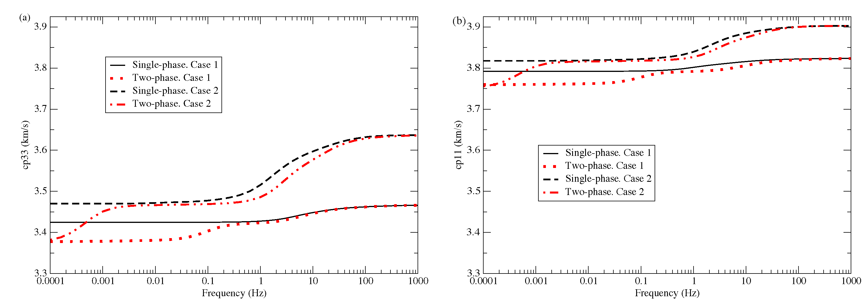
The following notation is used in the figures: cpII and $Q_{\mathrm{II}}=\mathrm{Re}\left(p_{\mathrm{II}}\right)/\mathrm{Im}\left(p_{\mathrm{II}}\right)$ are the phase velocity and dissipation factor of the waves traveling parallel and perpendicular to the layering, “11-waves” and “33-waves”, respectively.

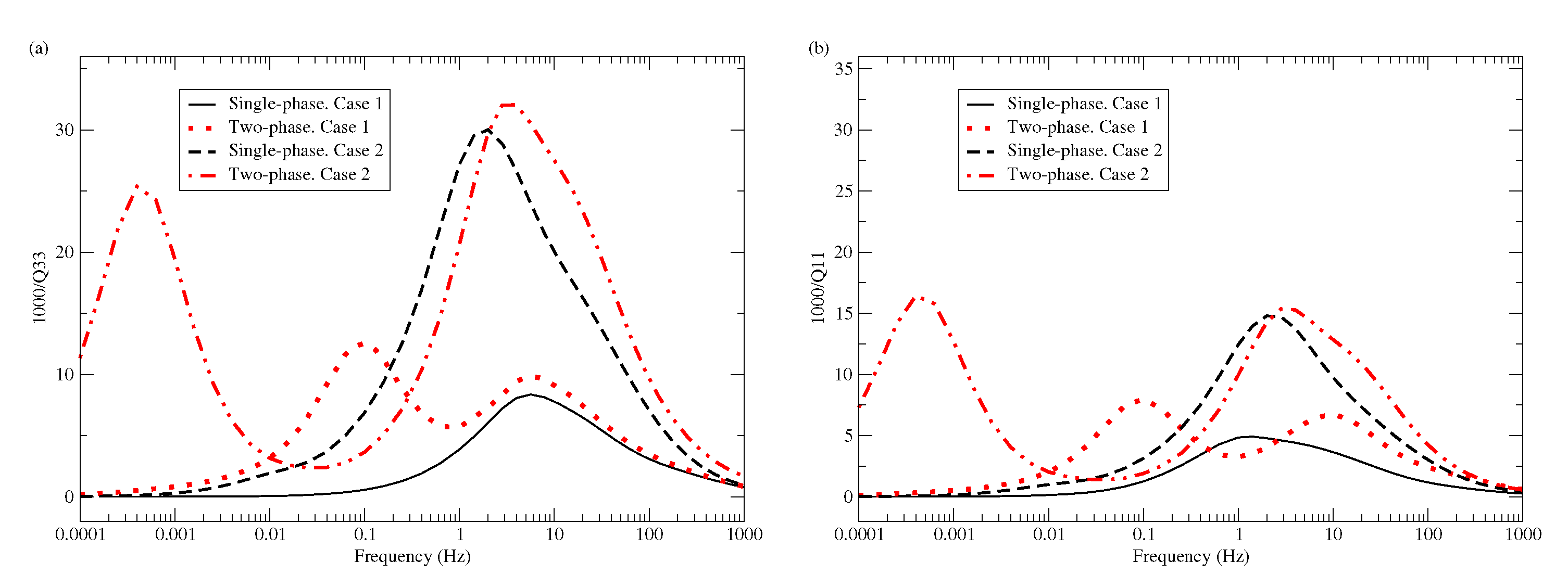
Figure 1a,b and Figure 2a,b show the phase velocities and corresponding dissipation factors of “33-waves” and “11-waves” as a function of frequency for Cases 1 and 2 computed with the FE method. The plots compare the results for two fluids and one (effective) fluid, where the latter is defined in Equations (42).

At low frequencies, the more realistic case of two-phase fluids has lower velocities than for single-phase fluids, with similar asymptotic values at higher frequencies. As expected, phase velocities for “33-waves” are lower than for “11-waves”.

The dissipation factors corresponding to two-phase fluids (Figure 2) exhibit a very different behavior as compared with the effective single-phase fluids, since there is an additional attenuation peak at lower frequencies, much stronger for Case 2. This new phenomenon can be explained as follows. Ignoring the cross-dissipative coefficient $d_{nw}$, the particle velocity of the l-phase $i\omega {\mathbf{u}}^l$, $l=o,g,b$ is equal to the gradient of the generalized fluid pressure ${\mathcal{T}}^l$ times the absolute permeability $\kappa$ and the l-phase mobility ${\gamma }_l\left(S_l\right)$, defined as ${\gamma }_l\left(S_l\right)=\left[K_{rl}\left({\overline{S}}_l\right)\right]/{\eta }_l$ [26]. For the values of brine, oil and gas saturation is used in the examples, at 1% (5%) oil saturation, and ${\gamma }_o$ is five (three) orders of magnitude lower than ${\gamma }_b$ and ${\gamma }_g$. Thus, fluid flows differently within the pore space, with the fluids interfering each other and inducing additional energy losses, which are not taken into account by the single-phase effective-fluid approach. Furthermore, Case 2 has more oil content than Case 1, thus inducing higher attenuation (see Figure 2). Moreover, the attenuation peaks for “33-waves” have higher amplitudes than for “11-waves”, a known effect in finely layered porous media. An additional result observed in the experiments is that, at a given saturation, varying the amplitude of the capillary pressure does not affect the attenuation.

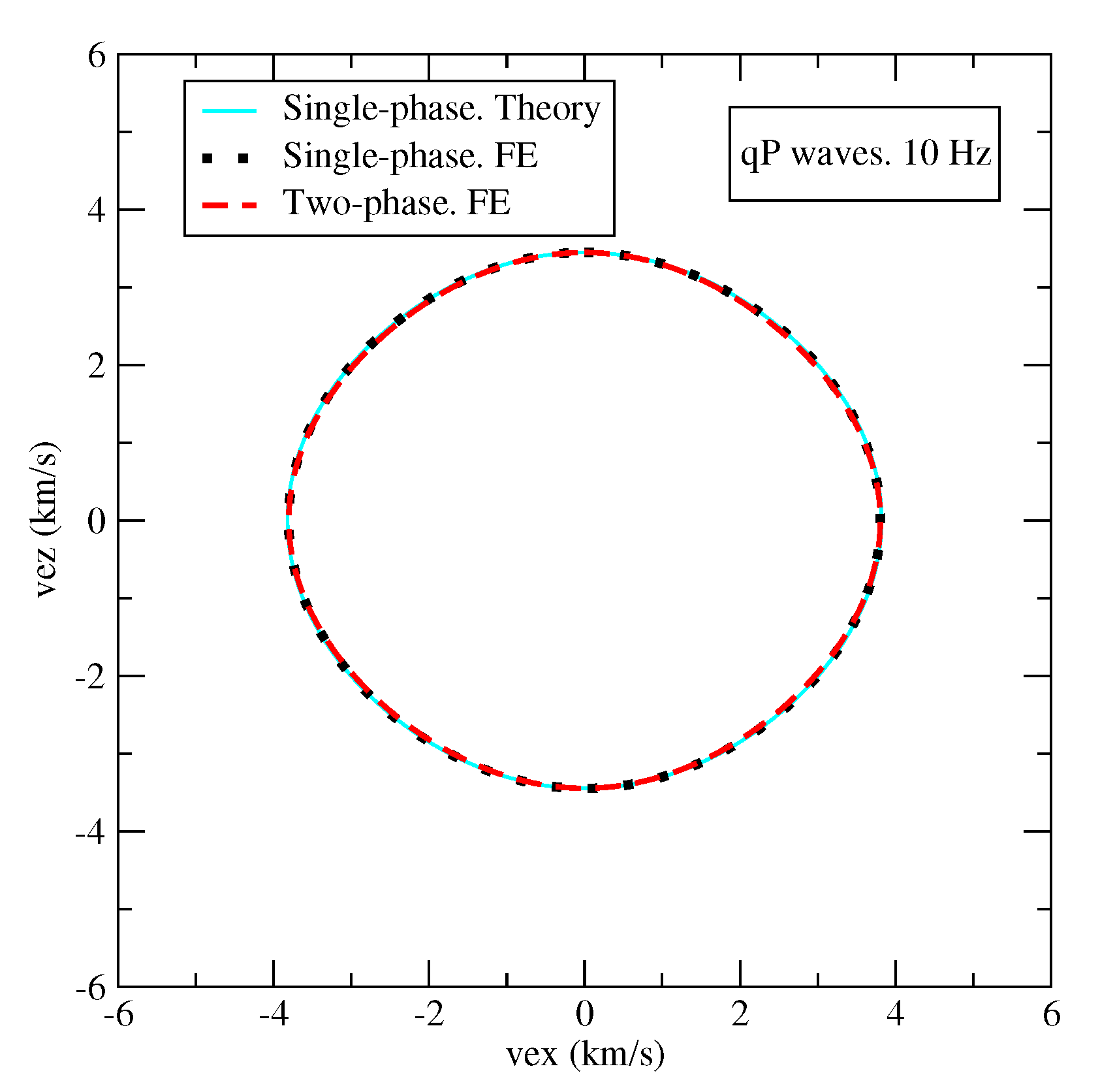
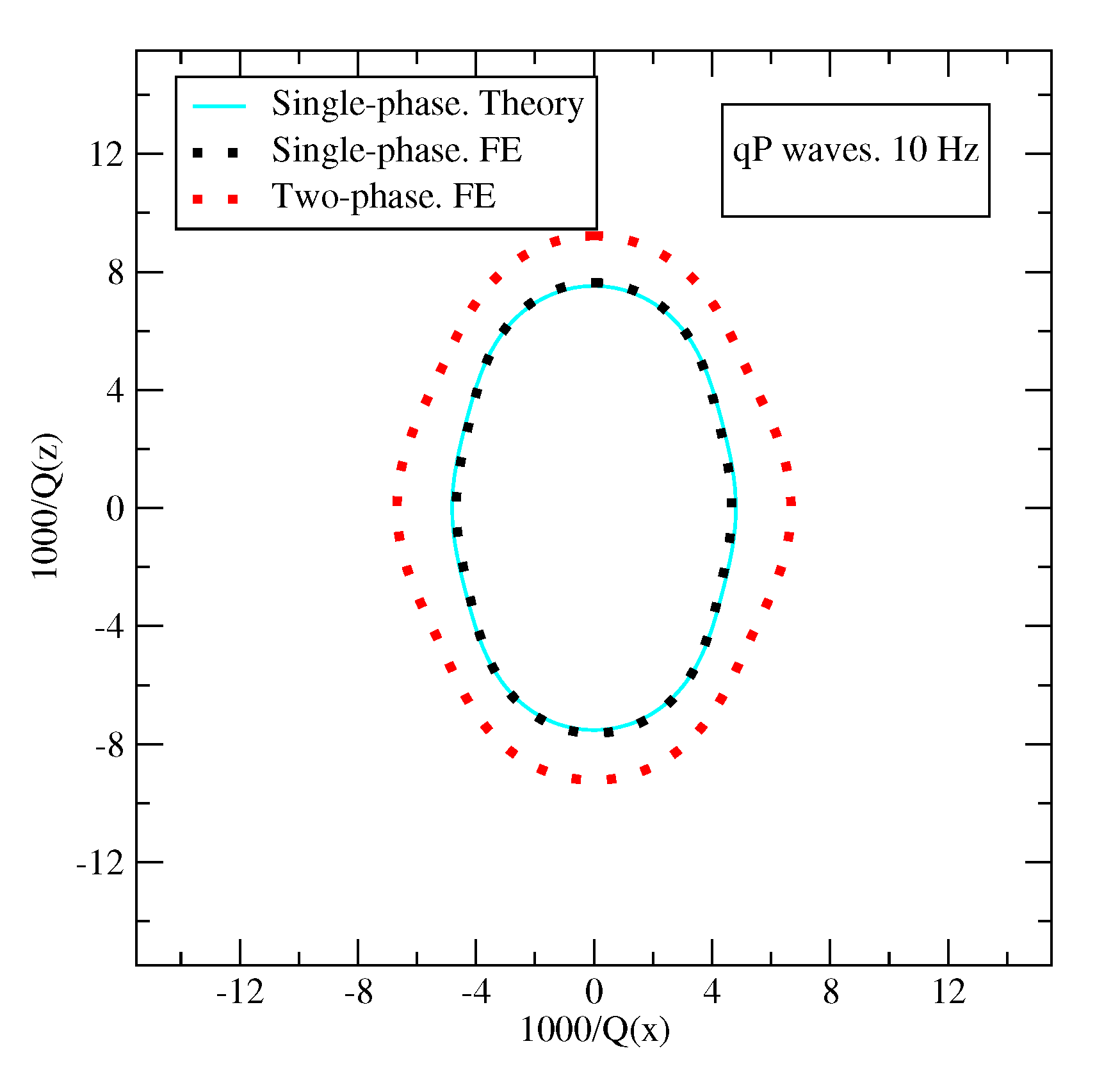
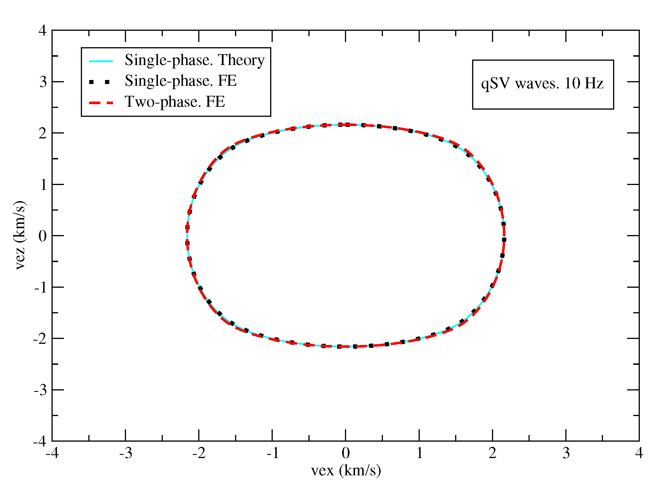
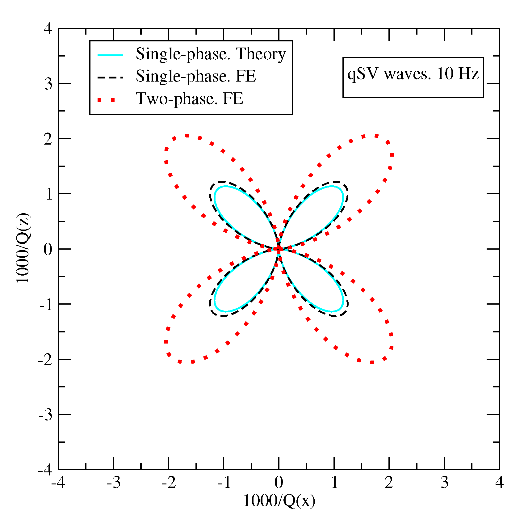
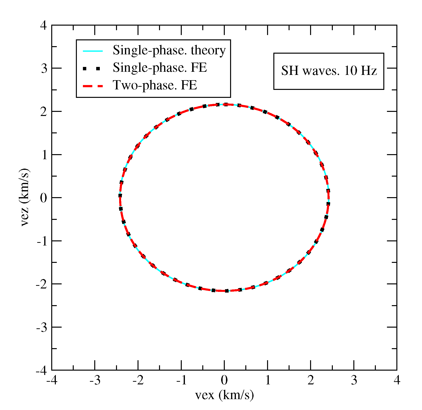
Figure 3, Figure 4, Figure 5, Figure 6 and Figure 7 exhibit polar plots of energy velocities and dissipation factors at 10 Hz versus the propagation angle. They compare analytical solution for single-phase effective fluids (Appendix B) to the FE solutions based on single-phase effective fluids and the two-phase fluids. Figure 3, Figure 5, and Figure 7 show that the energy velocities of the three waves have a perfect match, which validates the FE numerical scheme. On the other hand, Figure 4 and Figure 6 show a perfect agreement between the single-phase analytical and FE dissipation factors of the qP and qSV waves (SH waves are lossless), but the attenuation corresponding to the two-phase fluids, including capillarity effects, is higher, in agreement with the previous remarks regarding Figure 2.

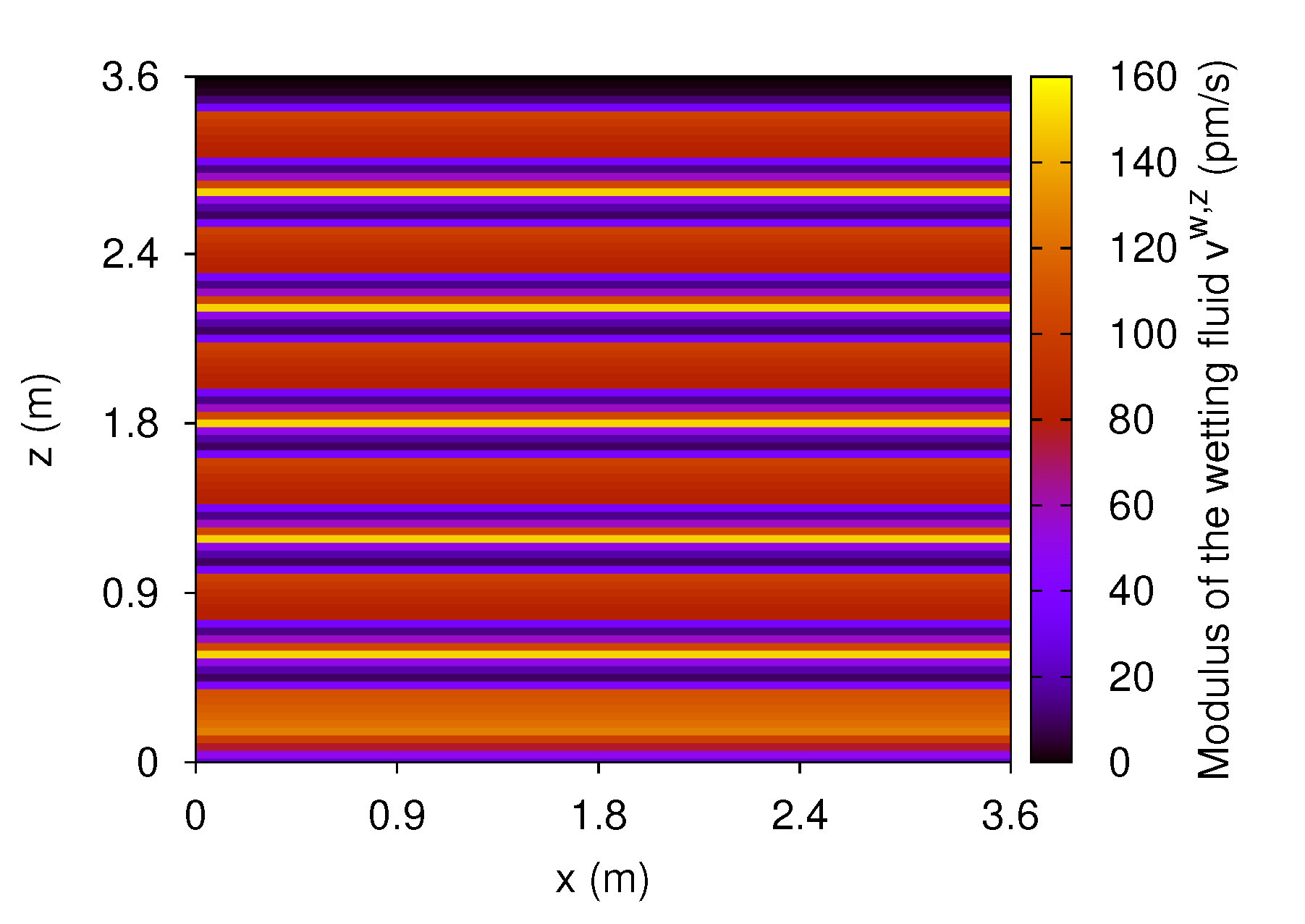
Figure 8 and Figure 9 display the modulus of the vertical component of the particle velocities ${\mathbf{v}}^w=\mathrm{i}\omega {\mathbf{u}}^w$ and ${\mathbf{v}}^n=\mathrm{i}\omega {\mathbf{u}}^n$ of the wetting and non-wetting fluids at 10 Hz, respectively, that appear in the left-hand side of the two-phase Darcy law (7) and (8). These vertical components, corresponding to Case 2, are denoted by $v^{n,z}$ and $v^{w,z}$ in the plots. The higher mobility ${\gamma }_b$, as compared with the gas and oil mobilities ${\gamma }_g$ and ${\gamma }_o$, explains the higher values of the wetting particle velocity in Figure 9 when compared with those of the non-wetting phase in Figure 8. As stated above, the interference between the two fluid phases due to their different particle velocities induces energy losses and velocity dispersion.

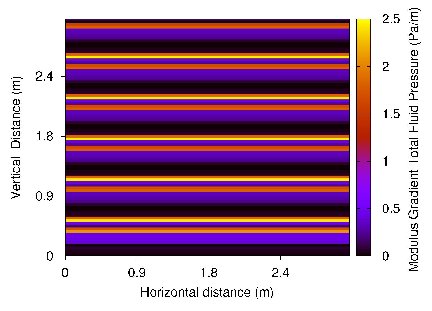
Finally, Figure 10 exhibits the modulus of the gradient of the total fluid pressure $\mathcal{T}={\mathcal{T}}_n+{\mathcal{T}}_w$ at 10 Hz for Case 2, which is clearly observed at the layer interfaces. This pressure gradient is another useful illustration of the WIFF mechanism for the case of two-phase fluid saturation.

5. Discussion

Wave-induced fluid flow in porous media is known to be a major cause of attenuation and velocity dispersion. Concerning the existence of additional slow waves when multiphase fluids saturate a porous medium, Albers [17] developed a macroscopic linear model to study wave propagation in unsaturated soils. This model, which assumes that capillary pressure and relative permeabilities depend on saturation, predicts the existence of three compressional waves, one of them fast and two slow, and a shear wave, with phase velocities and attenuation depending on saturation, and the coefficients in the stress-strain relations derived as in Reference [25].

Furthermore, Lo and Sposito [16] present differential equations to model dilatational waves in porous media saturated with two immiscible fluids. Their analysis predicts three compressional waves (P1, P2, P3), with the attenuation of the P1 wave highly affected by the pore fluids. On the other hand, the attenuation of the P2 and P3 waves is found to be related to the inverse of the sum of the relative mobilities of the two fluids, thus dominated by the fluid with larger relative mobility. This model also assumes that capillary pressure is a unique function of saturation (ignoring hysteresis), with the dissipation coefficients are defined in terms of the absolute permeability and the saturation-dependent relative permeability functions using the form given in Reference [25]. Quoting these authors “the model equations by Brutsaert [13], Garg and Nayfeh [14], Berryman et al. [15] and Tuncay and Corapcioglu [19] can be considered as special cases (of Reference [16]) and Santos et al. [25] (model) as a version based on a Lagrangian framework”.

6. Conclusions

Finite-element time-harmonic quasistatic experiments were used to study the wave anelasticity of a periodic set of three thin and flat layers saturated with two fluids, focusing on the effects of surface tension (capillarity forces). The results are compared with the case in which the two fluids are replaced by an effective single-phase one. This later case is validated against the analytical solution, whereas there is no analytical solution for the more general and realistic scenario involving capillary forces. The results show that, in this case, the loss is higher for both waves traveling normal and parallel to the layers, and there are two attenuation peaks, as opposed to one peak for the effective single-phase fluid.

The energy velocities and dissipation factors of the three waves, shown as polar plots at 10 Hz versus the propagation angle, exhibit a perfect agreement between the analytical and FE single-phase fluid solutions. While the energy velocities coincide in all cases, the dissipation factors are always higher for the case of two-phase fluids, as mentioned above. The physics can be explained by combined effects of capillary pressure and different mobilities of each fluid phase in the two-phase Darcy law.

The existence of an additional slow wave compared to the classic slow wave of the Biot theory is due to surface tension effects represented by a saturation-dependent capillary pressure. On the other hand, relative mobilities induce relative motions between the fluids, causing losses absent when an effective fluid is considered, as it is mostly the case in the literature regarding wave propagation in porous media. Future work includes a more detailed analysis of the influence of wettability, phase mobilities, and saturation on wave anelasticity of rocks saturated with immiscible fluids.