GHGs Emission from the Agricultural Sector within EU-28: A Multivariate Analysis Approach

Abstract

Climate mitigation and adaptation planning (CMAP) has recently been implemented across the EU-28 to reduce GHG emissions (CO₂, CH₄, N₂O). Thus, the aim of this study was to provide an overview of GHG emissions from the agricultural sector in the EU-28 from 1990 to 2019, and cluster the EU-28 countries regarding their total GHG emissions. The results emphasize the positive impact of CMAP through a negative trend of the total GHG emissions (−2653.01 thousand tons/year, p < 0.05). Despite the positive and not significant trend of the total CO₂ emissions, both CH₄ and N₂O exhibited a negative and significant trend. At the country scale, Italy, the United Kingdom, and the Netherlands showed the highest reduction in total GHG emissions, by −282.61thousand tons/year (p < 0.05), −266.40 thousand tons/year (p < 0.05), and −262.91 thousand tons/year (p < 0.05), respectively. The output of the multivariate analysis approach indicates changes in the pattern of GHG emissions between 1990 and 2019, where CO₂ emissions decreased in the case of Poland and Czechia. The output of this study highlights the positive impact of CMAP, adopted by EU countries, in minimizing GHG emissions. Despite some fluctuations in CO₂ emissions, strategies for attaining carbon neutrality in the agricultural sector, across the European Union, should be pursued.

1. Introduction

Rapid population growth and the concomitant increase in anthropogenic activities have resulted in climate change-induced challenges, and pose major threats to the sustainability of natural resources and the stability of the Earth’s biosphere, especially in the recent past [1]. These challenges are leading to uncontrolled accumulation of greenhouses gases in the Earth’s atmosphere [2]. The global concentration of greenhouse gas emissions (GHGs) has been accelerating particularly rapidly since the beginning of the industrial era because of various anthropogenic activities [3]; for instance, although the concentration of CO₂ in the 1760s was 280 ppm, the current estimate is 410 ppm, and is expected to reach 590 ppm by the end of 2100 [2]. The global tracking of greenhouse gas emissions provides a framework for assessing the contribution of individual countries to the climate change challenge. Climate change indicators define the emissions of the most significant GHGs from human activity, atmospheric concentrations, and how emissions and concentrations have evolved over time [4,5]. These indicators employ the concept of “global warming potential” for comparing the emissions of gases, in order to convert the quantities of other gases into CO₂ equivalents. The emissions of GHGs from human activities are rising and exacerbating climate change. This increasing level of GHGs is resulting in many more climate-related changes at the local to global scale [6].

Since the beginning of the industrial age, CO₂ and other GHGs in the atmosphere have been on the rise, primarily because of human activity. The net emissions of greenhouse gasses from human activities worldwide increased to 43% between 1990 and 2015. During this period, carbon dioxide emissions, representing approximately 35% of the total emissions, have grown by 51% [7]. The industrial and agricultural sectors accounted for 31.6% and 13.8%, respectively, and were considered to be major sources of GHG emissions, while 12.2% of the emissions came from land use changes [8]. Unpredictably, GHG emissions from the agricultural sector increased by 1.1% between 2000 and 2010 [9]. Many factors, such as agricultural expansion and/or intensification, deforestation, land clearing, fertilization, livestock production, and traditional soil management and cultivation, alter the global geochemical cycle and enhance GHG emissions from the agricultural sector, especially in developing countries [10]. Interestingly, Tian et al. [11] reported that 87% of the total N₂O emissions originated from the agricultural sector (71% agricultural + 16% N-fertilization), with cropland farming accounting for roughly 5% of all anthropogenic GHG emissions [12]. Therefore, many databases and analyses were developed to address the current and future contribution of the agricultural sector to climate change, and formulate adaptation and mitigation strategies. Politically, the assessment of GHG emissions from the agricultural sector, along with related sectors, such as forestry and other land use (i.e., AFOLU), will support the discussion about the role of agriculture in climate mitigation within the United Nations Climate Change Conference (COP26).

Recently, the GHG emissions from the European Union’s agricultural sector were estimated to be 10% of the total GHG emissions [13]. Although the total amount of EU-27 GHG emissions in 2019 was 4.065 MtCO_2e [14], the annual estimate of GHG emissions by agriculture was 436 million tons [15]. This suggests that energy is one of the main inputs in the agricultural system [16], whereas the energy from creating fossil fuels is mainly utilized by agriculture and multiple other actions, including forestry, which form 2.78% of the European Union correlated activities [17]. The Netherlands has the highest share of agricultural energy usage, with 8.1 percent, followed by Poland, which has 5.6 percent. In contrast, Romania accounts for the lowest percentage overall [18]. The growing quantity of energy is due to the neoteric agricultural activities, which are partly responsible for the persistent increase in GHG emissions [19]. About half of the energy used in the agricultural sector is derived from diesel and gas oil, which make up the highest share of energy utilized in the agricultural sector in the EU [15]. Regardless of the size and variation in the contribution of the agricultural sector in the national GDP in each member country of the EU, the EU has achieved a 23% reduction in GHG emissions in the last two decades [13].

Since its foundation, the EU has adopted many strategies, plans, and programs for environmental sustainability, with emphasis on energy management and the reduction in GHG emissions [20,21]. The common agricultural policy (CAP) is a policy created by the European Union, with the aim of implementing activities to integrate climate change reduction procedures into its policies [22]. During 2014–2020, over one hundred billion Euros, accounting for about 25% of the CAP budget, was the contribution of the commission to reduce, alleviate, and adjust to climate change. The European Green Deal strategy has recently been adopted, which is designed to promote climate neutral actions and resource-efficient consumption [20,23]. Many studies were carried out to assess low-carbon economy (LCE) within the agricultural sector. In view of this, Piwowar et al. [24] stress the importance of raising the awareness of farmers about LCE practice in rural areas of Poland. In Spain, Baccour et al. [25] suggested that a combination of measures could help reduce GHG emissions from the agricultural sector by 75%. Interestingly, Bajan et al. [20] proved that the usage of renewable energy in food production is approaching the expected strategic goals within V4 countries (Czechia, Slovakia, Hungary, Poland), resulting in some of the successes recorded in the reduction in GHG emissions from the agricultural sector in some EU countries (1990–2018). However, EU polices in agricultural sector led to a reduction of GHG emissions [26].

Promoting efforts towards minimizing GHG emissions at the field scale are required to attain the aspiration of GHG reduction in Europe by 2050 [27]. In addition to an efficient energy toolkit, water and carbon footprints for agriculture output are being established by the European Union. This is aimed at reducing water shortage, enhancing energy efficiency, and excluding gas emissions by 2050 [28]. The objectives laid out under the EU effort sharing law may vary slightly among member states, and there are exceptions, even though most EU member states do not have agricultural targets. The Netherlands, for instance, has established an emission reduction target of 3.5 MtCO₂eq yr⁻¹ by 2030, which should be reached by the co-funding of mitigation measures, and governmental and business cooperation in their National Agreement on Climate Change (NACC) [29]. Other member states have set carbon budgets in their national low-carbon strategy. France, for example, projected a cut in GHG emissions of 8% by 2023, 13% by 2028, and 20% by 2033, based on a benchmark of the 2015 levels [30]. The UK has also created carbon budgets that have strategic sector objectives, including a 20% reduction in agriculture, forestry, and other land use emissions from 2016 to 2030 [31]. In its 2050 climate action plan, Germany has more aggressive targets of reducing agriculture emissions by 31–34% in 2030, using a 1990 benchmark [32]. The climate action plan of Ireland provides a de-carbonization route to 2030, consistent with the adoption, by 2050, of net zero emission objectives [33]. There are some measures for reducing GHGs from the agricultural sector, such as cost-effectiveness analysis [34], reducing water consumption in different agricultural systems [35], no or reduced tillage (NT/RT) combined with crop rotations (i.e., legumes and cover crops) [36], and others [37,38]. On this basis, the objective of this study was to (1) evaluate the changes in GHG emissions from the agricultural sector of the EU-28 from 1990 to 2019, and (2) cluster the EU-28 countries regarding their total GHG emissions.

2. Materials and Methods

2.1. Data Collection

Data for the EU-28 countries between 1990 and 2019 were collected from the European Environment Agency (EEA) [39] (

Table 1. Type of collected data.

Data Type	Unit	Time Frequency
Total GHGs emission from agricultural sector *	Thousand tons	Annual
CO2	Thousand tons	Annual
CH4 (CO2 equivalent)	Thousand tons	Annual
N2O (CO2 equivalent)	Thousand tons	Annual

* Greenhouse gases (CO₂, N₂O in CO₂ equivalent, CH₄ in CO₂ equivalent, HFC in CO₂ equivalent, PFC in CO₂ equivalent, SF6 in CO₂ equivalent, NF₃ in CO₂ equivalent).

). These data were checked and updated in June 2021. All countries and their abbreviations are listed in Table 2.

2.2. Trend Analysis

Trend analysis could be conducted using parametric and non-parametric methods. Despite the effectiveness of parametric methods, they require independent and normally distributed data. In contrast, non-parametric methods simply require independent data [40]. In this research, the Mann–Kendall (MK) test [41,42] was used for detecting trend of GHGs across EU-28 countries. The MK is a well-known rank-based non-parametric test used to detect decrease (−) or increase (+) for studied variables through time. The advantage of using the MK test is that data do not have to be normally distributed, and they are not affected by outliers. The null hypothesis (H₀) in MK test states that there is no trend over time. For time series X = (X₁, X₂, … X_n), the static test of MK (S) could be interoperated as shown in Equations (1) and (2) as follow [41,42]:

$$\mathrm{S}={\displaystyle \sum }_{\mathrm{i}=1}^{\mathrm{N}-1}{{\displaystyle \sum }}_{\mathrm{j}=\mathrm{i}+1}^{\mathrm{N}}{\nabla }_{\mathrm{ij}}$$

(1)

$${\nabla }_{\mathrm{ij}}=\mathrm{sign}\left({\mathrm{x}}_{\mathrm{j}}-{\mathrm{x}}_{\mathrm{i}}\right)=\{\begin{array}{cc}1& {\mathrm{x}}_{\mathrm{j}}>{\mathrm{x}}_{\mathrm{i}}\\ 0& {\mathrm{x}}_{\mathrm{j}}={\mathrm{x}}_{\mathrm{i}}\\ -1& {\mathrm{x}}_{\mathrm{j}}<{\mathrm{x}}_{\mathrm{i}}\end{array}$$

(2)

where N: length of the data, ${\mathrm{x}}_{\mathrm{i}}$ and ${\mathrm{x}}_{\mathrm{j}}$: observations.

The variance in S is denoted as shown in Equation (3), as follows:

$$\mathrm{Var} \left(\mathrm{S}\right)=\frac{\mathrm{n}\left(\mathrm{n}-1\right)\left(2\mathrm{n}+5\right)-{\sum }_{\mathrm{i}=1}^{\mathrm{P}}{\mathrm{t}}_{\mathrm{i}}\left({\mathrm{t}}_{\mathrm{i}}-1\right)\left(2{\mathrm{t}}_{\mathrm{i}}+5\right)}{18}$$

(3)

where P: tied group, ${\mathrm{t}}_{\mathrm{i}}$: number of data. Then Z standard can be calculated. More details about MK calculations could be found in [40].

In this study the M_k was adopted for detecting the trend of GHG emissions to overcome the presence of outliers and skewed data [43]. Also, the Sen slope ($\mathsf{\rho }$) [44] was used to determine the amount of GHG changes per time. The ρ is a non-parametric method that captures the slope of the trend in a dataset (N pairs) as depicted in Equations (4) and (5), as follows:

$$\mathsf{\rho }=\frac{{\mathrm{x}}_{\mathrm{j}}-{\mathrm{x}}_{\mathrm{i}}}{\mathrm{j}-\mathrm{k}}\hspace{1em}\left(\mathrm{j}>\mathrm{k}\right)$$

(4)

where ${\mathrm{x}}_{\mathrm{j}},{ \mathrm{x}}_{\mathrm{i}}$ are values of the data. Then the median of $\mathsf{\rho }$ is computed as follows:

$${\mathsf{\rho }}_{\mathrm{median} }=\{\begin{array}{cc}{\mathsf{\rho }}_{\frac{\left(\mathrm{N}+1\right)}{2}}& \mathrm{if} \mathrm{N} \mathrm{is} \mathrm{odd}\\ \frac{{\mathsf{\rho }}_{(\frac{\mathrm{N}}{2})}+{\mathsf{\rho }}_{\frac{\left(\mathrm{N}+2\right)}{2}}}{2}& \hspace{1em}\mathrm{if} \mathrm{N} \mathrm{is} \mathrm{even}\end{array}$$

(5)

2.3. Multivariate Analysis

Principal component analysis (PCA) is a multivariate method for reducing a large number of inter-correlated quantitative data (dependent variables) to a smaller number of representative variables, known as principal components (PCs), by employing complex underlying mathematical functions [45,46]. In this study, the similarities and differences in GHG emissions (CO₂, CH₄ and NO₂) across EU-28 were determined using principal component analysis (PCA). The PCA was performed with the standardized approach using the correlation matrix to reveal the pattern of GHG emissions (CO₂, CH₄ and NO₂) in the ordination space defined by the principal components (PCs).

To show the differences between GHG emissions in 1990 and 2019, we conducted two PCAs by using biplots. Biplots can depict the cases considering the three dimensions with the correlations. We tested the model fit with the root mean square residual (RMSR), where values <0.1 are considered good and <0.05 indicated very good [47].

The EU-28 countries were divided into the following 6 groups: western (w) (Belgium, France, Luxemburg, the Netherlands, Ireland, the United Kingdom); northern (n) (Denmark, Finland, Sweden, Iceland); middle (m) (Austria, Germany); southern (s) (Greece, Spain, Italy, Cyprus, Portugal); post-socialist (Bulgaria, Estonia, Croatia, Latvia, Lithuania, Romania, Slovenia); and Visegrad 4s (v4) (Czechia, Slovakia, Hungary, Poland) based on their location and historical basis (having the heritage of communism on the economy). Using these groups, we tested the following hypothesis: H₀ that each group was from the same statistical population with the same medians using Kruskal–Wallis test. We performed the test with PCs of the PCA for the dataset of 1990 and 2019.

We also conducted a cluster analysis on the GHG emissions with the change, i.e., the ratio of 2019 and 1990 as percentages. We applied the Ward’s method and the output was visualized with a hierarchical dendrogram and in boxplot diagram.

3. Empirical Findings

3.1. Trend Analysis of GHGs Emissions between 1990 and 2019

3.1.1. Total GHGs Emissions between 1990 and 2019

The result of the MK test indicated that there was a significant decline in GHG emissions from the agricultural sector in the majority of the EU-28 countries (Figure 1,

Table 2. Trend analysis of GHG emissions and its component across EU-28 countries between 1990 and 2019.

EU-28 Countries		Total GHGs Emissions		CO2		CH4		N2O
		$\mathsf{\rho }$	MK	$\mathsf{\rho }$	MK	$\mathsf{\rho }$	MK	$\mathsf{\rho }$	MK
Total *	EU-28	<0.0001	−2653.01	0.42	−9.61	<0.0001	−1675.72	<0.0001	−916.06
Belgium	BE	<0.0001	−92.22	0.97	0.01	<0.0001	−31.48	<0.0001	−61.12
Bulgaria	BG	0.38	−22.62	0.00	0.57	<0.0001	−42.93	0.24	23.42
Czechia	CZ	<0.0001	−65.77	0.00	5.41	<0.0001	−65.89	0.70	−3.03
Denmark	DK	<0.0001	−78.51	<0.0001	−8.98	0.00	−7.76	<0.0001	−55.91
Germany	DE	0.00	−166.74	0.02	16.33	<0.0001	−177.53	0.83	5.06
Estonia	EE	0.72	3.00	0.40	0.14	0.83	−1.22	0.30	3.55
Ireland	IE	0.86	3.90	0.94	0.15	0.06	27.96	0.02	−22.92
Greece	EL	<0.0001	−73.27	<0.0001	−1.03	0.09	−6.02	<0.0001	−58.88
Spain	ES	0.34	66.99	0.32	1.69	0.92	9.10	0.05	52.44
France	FR	<0.0001	−227.20	<0.0001	9.17	<0.0001	−122.76	<0.0001	−109.34
Croatia	HR	0.00	−24.17	0.00	1.16	<0.0001	−16.16	0.00	−11.35
Italy	IT	<0.0001	−282.61	0.00	−5.26	<0.0001	−136.56	<0.0001	−143.50
Cyprus	CY	0.02	−2.37	<0.0001	−0.05	0.75	−0.11	0.00	−2.16
Latvia	LV	0.57	5.62	0.01	0.74	0.36	−4.73	0.04	7.97
Lithuania	LT	0.34	−7.94	0.34	0.19	<0.0001	−34.91	0.00	24.14
Luxembourg	LU	0.17	−0.91	<0.0001	0.17	0.34	0.51	<0.0001	−1.61
Hungary	HU	1.00	0.07	0.18	2.44	<0.0001	−33.08	<0.0001	37.97
Malta	MT	<0.0001	−1.18	-	-	<0.0001	−0.82	<0.0001	−0.37
Netherlands	NL	<0.0001	−262.91	0.01	−0.99	0.00	−92.96	<0.0001	−173.15
Austria	AT	0.00	−27.57	<0.0001	2.70	<0.0001	−21.41	0.00	−7.01
Poland	PL	0.00	−216.02	<0.0001	−33.94	<0.0001	−137.11	0.03	−36.94
Portugal	PT	0.00	−24.21	0.83	0.03	0.00	−14.47	0.01	−10.32
Romania	RO	<0.0001	−257.30	0.13	0.77	<0.0001	−187.77	0.02	−72.44
Slovenia	SI	0.00	−3.55	<0.0001	−0.81	0.18	−1.04	0.00	−1.56
Slovakia	SK	<0.0001	−43.52	0.42	0.54	<0.0001	−40.52	0.48	−3.10
Finland	FI	0.00	−11.64	<0.0001	−11.44	0.01	−3.27	0.14	2.70
Sweden	SE	<0.0001	−32.85	0.02	−1.05	<0.0001	−18.21	<0.0001	−15.46
Iceland	IS	0.46	0.27	0.00	0.13	0.13	−0.45	0.02	0.49
United Kingdom	UK	<0.0001	−266.40	0.17	8.47	<0.0001	−161.26	<0.0001	−115.55

* (2013–2020).

). Table 2 shows that 20 European countries, Belgium (BE), Czechia (CZ), Denmark (DK), Germany (DE), Greece (EL), France (FR), Croatia (HR), Italy (IT), Latvia (LV), Malta (MT), the Netherlands (NL), Austria (AT), Poland (PL), Portugal (PT), Romania (RO), Slovenia (SI), Slovakia (SK), Finland (FI), Sweden (SE), and the United Kingdom (UK), had significant (p < 0.05) negative trends. The GHG emission trends were negative, but not significant, in Bulgaria (BG), Cyprus (CY), Lithuania (LT), Luxembourg (LU), and Iceland (IS). In contrast, positive, but not significant, trends were recorded in Estonia (EE), Ireland (IE), Spain (ES), and Hungary (HU).

The highest reduction in GHG emissions was recorded in IT (−282.61 thousand tons/year, p < 0.05), followed by the UK (−266.40 thousand tons/year, p < 0.05), and NL (−262.91 thousand tons/year, p < 0.05). The lowest reduction was recorded in MT (−1.18 thousand tons/year, p < 0.05), and SI (−3.55 thousand tons/year, p < 0.05). Nonetheless, the total emissions from the EU-28 depicted a significant reduction by −2653.01 thousand tons/year.

3.1.2. CO₂ Emissions between 1990 and 2019

The majority of the EU-28 countries exhibited a positive CO₂ emissions trend from the agricultural sector between 1990 and 2019 (Figure 2, Table 2). Only a few countries showed a negative significant trend, e.g., DK (−8.98 thousand tons/year, p < 0.05), EL (−1.03 thousand tons/year, p < 0.05), IT (−5.26 thousand tons/year, p < 0.05), CY (−0.05 thousand tons/year, p < 0.05), NL (−0.99 thousand tons/year, p < 0.05), PL (−33.94 thousand tons/year, p < 0.05), SI (−0.81 thousand tons/year, p < 0.05), FI (−11.44 thousand tons/year, p < 0.05), and SE (−1.05 thousand tons/year, p < 0.05). In contrast, some EU countries exapted a positive significant trend, such as BG (+0.57 thousand tons/year, p < 0.05), CZ (+5.41 thousand tons/year, p < 0.05), DE (+16.33 thousand tons/year, p < 0.05), FR (+9.17 thousand tons/year, p < 0.05), HR (+1.16 thousand tons/year, p < 0.05), LU (+0.17 thousand tons/year, p < 0.05), AT (+2.7 thousand tons/year, p < 0.05), and IS (+0.13 thousand tons/year, p < 0.05). Nonetheless, the rest of the EU countries showed positive, but not significant, trends (Table 2).

3.1.3. CH₄ Emissions between 1990 and 2019

The total emissions of CH₄ from the agricultural sector decreased significantly across the EU-28 (Table 2, Figure 3). The highest significant reduction was recorded in RO (−187.77 thousand tons/year, p < 0.05), DK (−177.53 thousand tons/year, p < 0.05), the UK (−166 thousand tons/year, p < 0.05), and PL (−137.11 thousand tons/year, p < 0.05). Despite the negative significant changes in CH₄, some countries, e.g., EE, CY, LV, SI, and IS, exhibited a negative, but not significant, trend. Notably, apart from IE (+27.96 thousand tons/year, p > 0.05), ES (9.10 thousand tons/year, p > 0.05), and LU (0.51 thousand tons/year, most of the EU-28 countries witnessed a negative trend of CH₄ emissions (p > 0.05) (Table 2, Figure 3).

3.1.4. N₂O Emissions between 1990–2019

Similarly to CH₄ emissions, N₂O emissions exhibited a negative trend from most of the EU-28 countries (Table 2, Figure 4). The total reduction in N₂O emissions from all the EU-28 countries was −916 thousand tons/year (p < 0.05) (Table 2). However, some countries showed a significant positive trend of N₂O emissions; for instance, LV (+7.79 thousand tons/year, p < 0.05), LT (+24.14 thousand tons/year, p < 0.05), HU (+37.97 thousand tons/year, p < 0.05), and IS (0.49 thousand tons/year, p < 0.05). On the other hand, some other countries, such as BG (+23.42 thousand tons/year, p > 0.05), DE (+ 5.06 thousand tons/year, p > 0.05), EE (+3.5 thousand tons/year, p > 0.05), ES (+52.44 thousand tons/year, p > 0.05), and FI (2.7 thousand tons/year, p > 0.05), showed a positive, but not significant, trend in N₂O emissions. Interestingly, the other EU countries showed a significant negative trend of N₂O emissions, whereas the highest value of reduction was recorded in NL (−143.5 thousand tons/year, p < 0.05), followed by IT (−143.5 thousand tons/year, p < 0.05), then the UK (−115.55 thousand tons/year, p < 0.05).

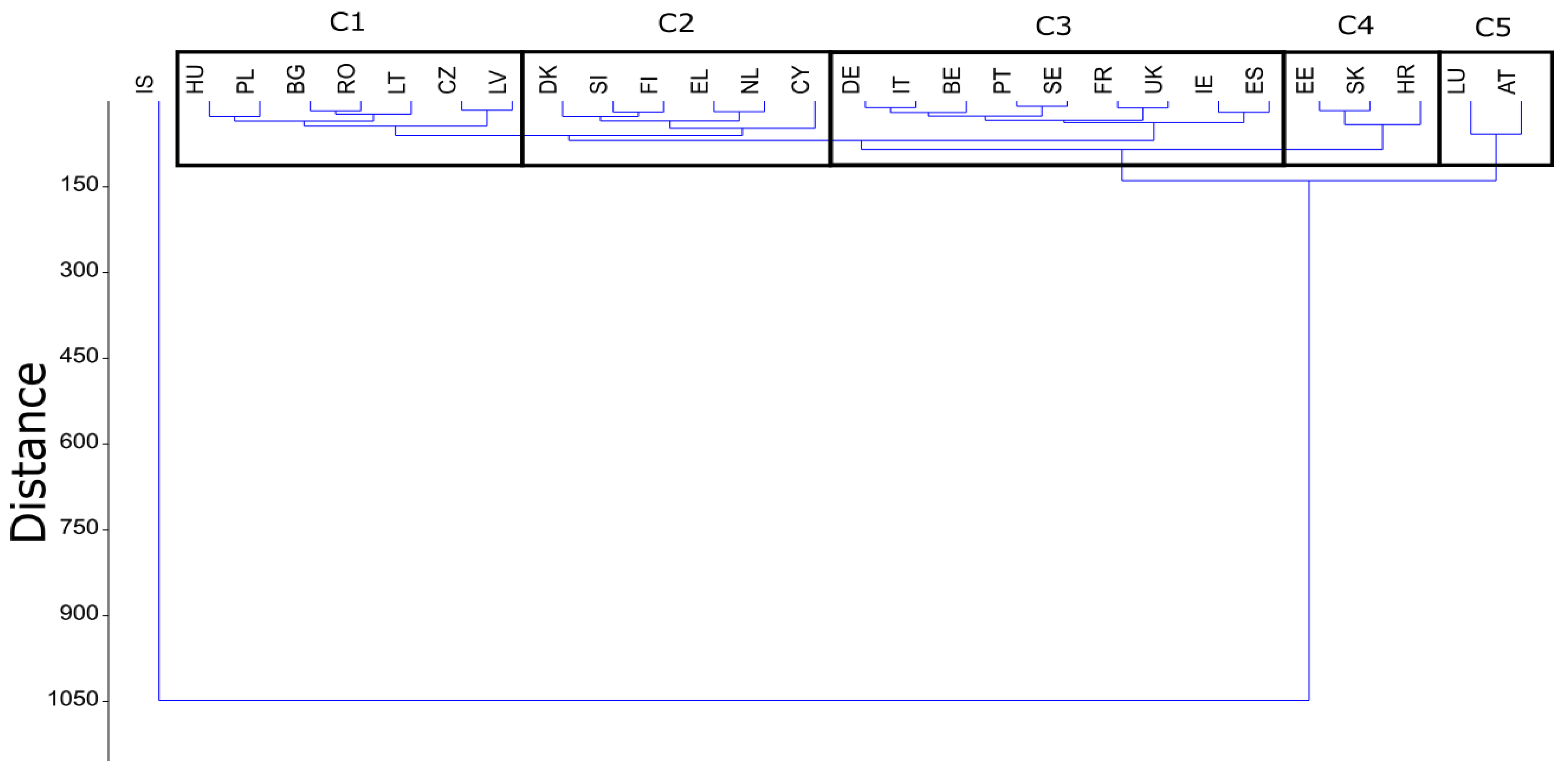
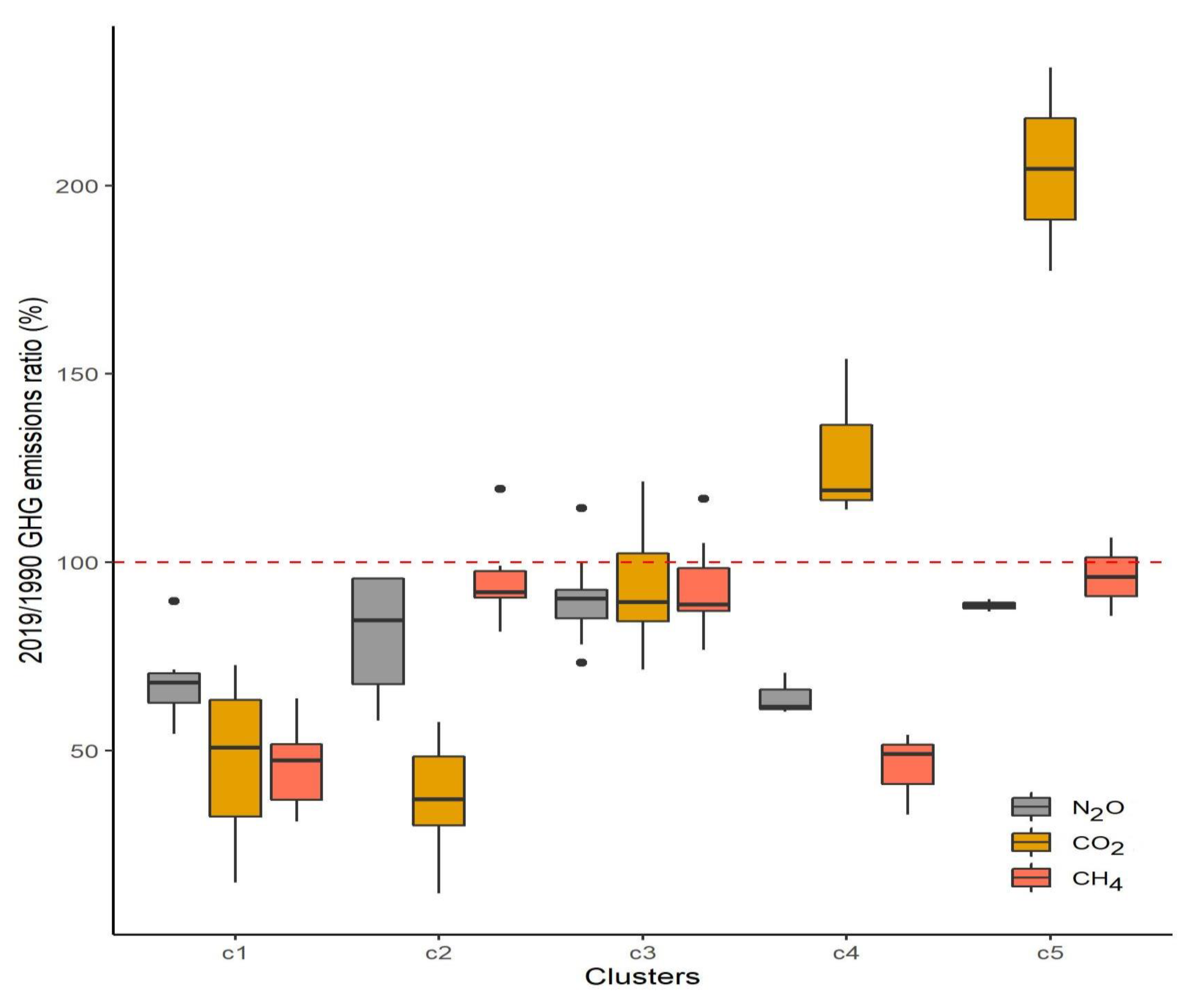
3.2. Multivariate Analysis of GHGs Emissions in 1990 and 2019

The total variance explained was 99% for the data of 1990 and 98% for 2019. Goodness-of-fit analysis also indicated a very good fit, with RMSRs of 0.01 for both years. Two PCs were confirmed by the RMSRs; PC1 correlated with the N₂O and CH₄ emissions, explaining 58% (in 1990) and 51% (in 2019) of the variance, while PC2 correlated with CO₂, and explained 41% (in 1990) and 46% (in 2019) of the variance. Consequently, PC2 involved only one variable, CO₂, while PC1 followed the state of N₂O and CH₄ on the same axis.

Most countries formed a compact group in both years in the lower section of the diagram, regarding N₂O and CH₄, and with a larger variance in CO₂. There were also outlier countries (having scores larger than two) regarding the lower or higher GHG emissions (Figure 5). In 1990, DE, FR, the UK, and PL represented the highest emissions of N₂O and CH₄, and CZ, PL, and DE had larger emissions of CO₂. The lowest CO₂ belonged to RO, FR, IT, and ES. The scores were mainly between −1 and 1 regarding the CO₂; thus, the variance was smaller than what was observed in PC2 (N₂O and CH₄). There were changes in the pattern in 2019, but the most important ones were observed in the lowest and largest values. The positions regarding PC1 (i.e., N₂O and CH₄) did not change, but the CO₂ emission decreased in PL and CZ, and increased in the UK, DE, and FR. The lowest CO₂-emitting countries were ES, IT, and NL.

There were no significant differences regarding PC1 in 1990 (Kruskal–Wallis H: 8.334, p = 0.138) and in 2019 (Kruskal–Wallis H: 6.654, p = 0.254). Similarly, there was no significant difference in CO₂ emissions in 1990 (Kruskal–Wallis H: 9.973, p = 0.076) and in 2019 (Kruskal–Wallis H: 10.59, p = 0.052). Accordingly, the spatial distribution of the countries did not discriminate the emissions.

Cluster analysis, focusing on the positive and negative changes, revealed that the difference was the most discriminative in the case of Iceland, due to its high increase in CO₂ emissions. Other clusters were only partly formed by their location (e.g., southern or western), and the differences were relatively smaller than those observed in Iceland. As Iceland formed a unique cluster in itself, we did not involve it in the statistical evaluation. Cluster 1 (C1) was formed by purely post-socialist countries, but all the other clusters were a mixture of different locations and historic heritage (Figure 6). This approach maximized the variance among the countries; thus, the clusters reflected similarity in the changes (Figure 7).

The C1 cluster contained the countries that had the largest negative change, i.e., these countries made the largest progress in reducing GHG emissions. The countries of the C2 cluster gained relevant results on decreasing CO₂ and CH₄, and the N₂O emissions also decreased, but by a smaller measure. In the C3 cluster, the countries only reached a small decrease in each GHG, and a limited increase was observed for CO₂. In both the C4 and C5 clusters, the CO₂ emissions increased, while the N₂O and CH₄ emissions decreased; the difference between the two clusters was that in C5, the decrease was smaller.

4. Discussion

In general, the trend of GHG emissions from the agricultural sector in EU countries was negative during 1990–2019, except for some countries, such as Estonia, Ireland, and Latvia, which displayed a slight increase from 3–5.6 thousand tons/year. Iceland and Hungary both exhibited insignificant increases. A significant increase in GHG emissions was exhibited by Spain (Figure 1), with a significant increase in N₂O emissions (Figure 4). In fact, more than 72% of the Spanish land was used for agricultural practices and forestry, while 19% was used for meadows, which accelerated the GHG emissions from this sector [48,49]. Nonetheless, 11% of the total emissions in Spain originated from the agricultural sector [50]. The increase in GHG emissions in Spain, between 1990 and 2019, could be attributed to the lack of clear national strategies for minimizing and mitigating GHG emissions from the Spanish agricultural sector [51] (Table 2). This was exacerbated by the highly intensive agricultural production per capital and technological advancements in the agricultural sector in Spain in the recent decades [52]. The significant positive trend of GHG emissions was mainly dependent on the increase in N₂O emissions from 1990 to 2019, with an overall trend of 52.44 thousand tons/year. This trend may be because of the mismanagement of soil fertilization, agrochemicals. Livestock manure was the main cause of N₂O emissions, eutrophication of water courses, and atmosphere acidification. Similar conclusions have been reported by Albiac et al. [52] and other workers [53,54]. Magrama [55] noted that the overdose of N fertilizer, along with the neglect of livestock manure, added more than 780.000 tN of fertilizer to the soil, leading to severe environmental pollution. Nevertheless, the mean annual increase in CH₄ and CO₂ emissions during the period of this study showed much lower values of 9.10 and 1.69 thousand tons/year, respectively. Other countries, such as Italy, the Netherlands, the UK, among others, manifested a significant decline in the total GHG emissions.

In Italy, only 7.1% of the GHG emissions originated from the agriculture sector in 2016. The decline in GHG emissions can be attributed to a decrease in the number of animals, especially the dairy cattle heads from 1990 to 2016, which resulted in a decline of about 40% [56]; this may have contributed to the negative trend of CH₄ emissions (Table 2 and Figure 3). Also, the CH₄ and N₂O from manure management decreased with the decline in the number of animals during the studied period. The more efficient manure management system may have also contributed to the reduction in N₂O [56]. The CH₄ emissions from rice cultivation have also decreased, according to the revised CH₄ daily EF measurements in Italian rice fields [57,58], considering the different agronomic practices between the different cultivars [59,60], and the different irrigation regimes [61]. The N₂O emissions from managed soils declined from 29.72 Gg (80.6% of N₂O emissions for the agriculture sector) in 1999 to 23.99 Gg (78.2%) in 2016, where this decline agreed with Table 2 and Figure 4. The decline in the N₂O emissions from managed soils may be because of a reduction in the use of inorganic and organic fertilizers, which was about 25% from 1990 until 2016 [56]. Romano et al. [56] reported that the application of carbonate for decreasing soil acidity is one of the main sources for CO₂ emissions. In this context, the liming process in Italy was responsible for 2.3% (2016) of the total CO₂ emissions from the agricultural sector [56].

The agricultural sector in the UK accounted for 10% (2018) of the GHG emissions [62], where livestock and manure accounted for 56% of the emissions, synthetic fertilizers accounted for 31%, and fuel and machinery accounted for 12% [62]. There was a significant decline in CH₄ and N₂O emissions in the UK during the studied period, with values of −166 thousand tons/year, p < 0.05, and −115.55 thousand tons/year, p < 0.05, respectively; this resulted in a decline in the total GHG emissions, with a trend of −266.40 thousand tons/year, p < 0.05 (Table 2). Similarly, Nair et al. [63] and NFS [64] reported that, overall, the GHG emissions from agriculture in the UK have decreased by 16% from 1990 to 2018. Ortiz et al. [62] mentioned three factors that led to a significant GHG emission decrease from the agricultural sector. The factors are as follows: (1) adaptation of new technology in the agricultural sector, (2) national policies, and (3) changing the incentives model, which reduced the number of ruminants to meet the EU-CAP (Common Agricultural Policy). The UK have launched a national framework for evaluating the annual reduction in GHG emissions since 2012. This framework covers ten indictors, including mitigation and adaptation methods, farmer knowledge and behavior, and emission per product [65]. It is good to mention here that a large amount of research in the UK was focused on the improvement in the agricultural GHG inventory [65]. The livestock population in the UK reduced by 19.8% from 1990 to 2018, while only the dairy cattle category also decreased by 33.6%. The application of N fertilizer had been dropped by permanent grasslands, which represented almost half of the area of the UK’s major crop area, with 55.6% from 1990 to 2018, while the other crops have been fluctuating between declining, such as by grass leys, oilseed rape, and potatoes, with 41%, 19%, and 27.2%, respectively; stabilizing, such as by wheat; and increasing in N fertilizer, such as by Spring and Winter barely, with 15.6% and 10%, respectively [66].

Studies indicate that liming is a major contributor to CO₂ emissions in the agricultural sector. The contribution of the agricultural sector to GHG emissions in the Netherlands was about 9.7% in 2019. There was a reduction in the application of lime, which also caused a reduction in CO₂ emissions during 1990–2008 and 2016–2019 in the Netherlands, although there was a slight increase in emissions in 2009. The reduction in liming resulted in the decline of CO₂ emissions, by 80.9%, from 1990 to 2019 (0.18–0.03 Tg CO₂ eq), while the CO₂ emissions from urea application increased from 0.002 to 0.045 Tg CO₂ eq in the same period [67]. This behavior explained the results of the CO₂ emissions of NL (Figure 2 and Figure 3, and Table 2). The trend of methane during the studied period decreased because of a reduction in the application of mature dairy cattle, where the CH₄ emissions of enteric fermentation and manure management decreased from 1990 to 2005, increased from 2007 to 2016, then start to decrease again [67]. The significant negative trend of N₂O emissions in NL (Figure 4) is explained by the decrease in organic and inorganic N fertilizer application, the decrease in animal numbers, and the decrease in animal production on pasture, from 1990 to 2010, and, after 2010, the decline in N₂O emissions was stabilized at 44.8% (8.7–4.8 Tg CO₂ eq). This is similar to the decrease in N₂O from the agriculture soil reported by Ruyssenaars et al. [67].

For Romania, a number of measures have contributed to the reduction in GHG emissions, such as minimizing the amount of synthetic nitrogen fertilizer, decreasing the number of livestock, and reducing the area under rice cultivation [68]. The Romanian agricultural sector contributed 18.98% (2015) to the total GHG emissions [68]. Compared to 1989, the reduction in GHG emissions reached 78.93% by liming, 72.98% by rice cultivation, 61.86% by manure management, 49.20% by enteric fermentation, 48.48% by agricultural soils, 46.34% by urea application, and 12.84% by the field burning of agricultural residues [68]. These findings agreed with the negative trend of Romania in Table 2 and Figure 1, Figure 2, Figure 3 and Figure 4. Table 2 shows that the negative trend of CH₄ was the highest, −187.77 thousand tons/year, followed by N₂O emissions with a negative trend, −72.44 thousand tons/year.

The total share of GHG emissions from agriculture in 2017 in Poland was 7.16% [69]. However, Poland showed a significant decline in the agricultural GHG emissions from 1990 to 2019, with a trend of −216.02 thousand tons/year (p < 0.05), which was categorized into −33.94 thousand tons/year (p < 0.05), −137.11 thousand tons/year (p < 0.05), and −36.94 thousand tons/year (p < 0.05) for the CO₂, CH₄, and N₂O emissions (Table 2), respectively. Poland’s National Inventory Report [69] stated that the decline in CH₄ emissions was due to the dramatic decrease in the livestock population after 1989, especially for the dairy cattle population that decreased by almost 50% from 1990 to 2017. This decline in the livestock population decreased the CH₄ emissions for enteric fermentation and manure management. As well as this, the N₂O emissions from manure management dropped by 31% from 1988 to 2017, also depending on the diminishing livestock population. N₂O emissions mainly come from the agriculture soil, which was significantly decreased from 1988 to 2017, by 21%. However, nitrogen fertilization accounted for 47% of direct N₂O emission (2017). Piwowar [70] explained that the liming process and carbonate usage were balanced from 2000 to 2004, and were relatively low later on. The CO₂ emissions from lime, dolomite and urea utilization were significantly decreased from 1988 to 2017 [69].

French agriculture GHG emissions contributed 16.8% of the total GHG emissions in 2019 [71]. France accounts for 25% of the livestock in Europe, and 40% of the agricultural land in France is used for cereal production, making France the largest producer of cereal in the EU [72]. The large proportion of livestock and cereal production in France also implies that France will account for a large part of the GHG emissions, and will have a difficult challenge in reducing GHGs. However, there was a significant decline in CH₄ emissions resulting from livestock (Table 2). The National Inventory Report for France [71] noted that a 34% decline in the dairy cattle population resulted in a 13% decrease in enteric fermentation emission from 1990 to 2019. An increase in the number of pig herds has been linked to an increase in manure management and a 7% increase in CH₄ emissions over the period 1990–2019. However, other parameters, such as the increase in manure management systems in the form of slurry, are contributing inversely to this trend. Rice cultivation is also a major contributor to CH₄ emissions. The area under rice cultivation in 1990 was 22,458 ha. This increased to 34,405 ha in 1994, but has declined to 15,100 ha in 2019. A decrease in the area under rice cultivation results in a decrease in rice cultivation-induced CH₄ emissions. Table 2 shows that the N₂O emissions also decreased significantly during 1990–2019. The National Inventory Report for France [71] indicated a decrease in N₂O emissions by minimizing the use of mineral nitrogen fertilizers, which reduced the N₂O emissions by −16% (1990–2019), and decreasing the cattle herds, resulting in a reduction in both the nitrogen excreted in the pasture and the organic nitrogen to be applied, leading to a 12% decline in N₂O emissions from 1990 to 2019. The total N₂O emissions from agricultural soils decreased by −9% over the period 1990–2019 (Table 2).

In Germany, the agriculture sector was responsible for 7.6% of the total GHG emissions in 2019 [73]. The total GHG emissions from the agricultural sector decreased by 19.2% in the period 1990–2021 [74]. This decline is consistent with the negative trend in Table 2 )−166.74 thousand tons/year, p < 0.05), which mainly depends on the CH₄ emissions trend that revealed −177.53 thousand tons/year (p < 0.05) (Table 2). As mentioned before, the CH₄ emissions come from enteric fermentation and manure management, and both rely the most on the population of animals, especially the dairy cattle, and pig for manure management. The German NIR [75] reported that, from 1990 to 2019, the decline in the animal population was almost 37%, 42%, 18.5%, and 41.6% for the dairy cattle, swine, sheep, and goats, respectively. This notable decline in the animal population leads to a decrease in CH₄ emissions, by 27.7% and 21.3% for enteric fermentation and manure management, respectively [74] (Table 2 and Figure 3). The N₂O emissions include manure management, energy crops (from digester and storage of digestate from the anaerobic digestion of energy crops, and include both CH₄ and N₂O emissions), and agricultural soil. In regards to the emissions from energy crops (CH₄ and N₂O), which presented the smallest share of the total agricultural GHG emissions (2.5% in 2019), they increased from zero in 1990 to 1573 Tg CO₂ eq in 2019, with a gradual utilization of energy crops since 1991. The N₂O emissions decreased by 18.9% for manure management and 15.3% for agricultural soil. The smaller dwindling of N₂O emissions from 1990 to 2019 may be attributed to variation in its components’ behavior (decrease in mineral fertilizer N quantities by 35%, decrease in manure N quantities, including energy crops, by 18.6%, increase in crop residues N quantities by 16%, and the relatively unchanged indirect soil emissions) [74,75]. In contrast, our results indicate a positive, but not significant, trend of N₂O (Table 2). The reasonable cause of that could be the increase in the applied N fertilization quantities between 2014 and 2016. The CO₂ emissions trend exhibited an increase, with a positive trend (16.66 thousand tons/year (p > 0.05)) (Table 2, Figure 2). Similar results were reported by the German NIR [75], which highlighted a 10.68% and 8.8% increase in the application of limestone and urea, respectively, and a decrease in the application of dolomite and calcium ammonium nitrate (84.5% and 61.6%, respectively). This resulted in a total increase in CO₂ emission from 1990 to 2019, by 11.6% [74].

The highest share of GHG emissions in the agricultural sector is presented by the CH₄ and N₂O emissions, accounting for more than 90% of the total GHG emissions. This majority share explained the clear proximity of the CH₄ and N₂O emission values of the contributing countries to the PC1 (Figure 5), where CH₄ and N₂O emissions, which are the closest components to PC1, best approximate the total GHG emissions. Nevertheless, the CO₂ emission values with a lower share of GHG emissions, and sometimes with opposite behavior to the total GHG emission values, were close to PC2. However, analysis of the spatial pattern, or even the historical heritage (post-socialist shared heritage on the agriculture, with the transformation from large agricultural co-operations to private farming), did not reveal any result. There were exceptions in each group; thus, the differences were not significant in the change between 1990 and 2019. The biplots pointed out countries that had increasing or decreasing changes during the 29 years. Furthermore, cluster analysis was the best method to show the country groups of similar changes, but, in this case, we involved the ratio of the change in the GHG emissions between the earliest and latest dates, dividing the data of 2019/1990. This approach was an efficient tool to identify the countries that have similar gains in GHG emission reduction, or in pointing out the ones that have issues in reaching the goals.

Iceland formed a sole cluster, but we have to highlight that the cause of this was the 1128% surplus in the CO₂ emissions from agricultural sources. This seems to be a large increase, but in 1990, the initial emissions were only 0.52 thousand tons, the smallest in the EU countries; even Luxembourg and Cyprus could approach it (with 6.3 and 1.8 thousand tons). In 2019, the CO₂ emissions of Iceland increased to 5.87 thousand tons, which was the second lowest in the EU, and Cyprus was the first, with 0.22 thousand tons in this year. In 2021, the world’s first CO₂ removal plant started operating in Iceland, which will remove 4000 t of CO₂ a year [76]. Austria and Luxembourg formed the cluster, both having the worst performance, but the increase should also be evaluated carefully; Luxembourg is still third in the ranks of CO₂ emissions in the EU. Accordingly, the countries that had the smallest emissions in 1990 can appear as inefficient ones in CO₂ reduction, but there are lot of components of these numbers. Besides local food production, transportation and even food import can also count, and can have direct consequences on the emissions too [77]. Although the population did not increase in the European countries, globalization can generate demands and, therefore, food or agricultural product import and export. In the case of Iceland, the food product import was USD 268,000 in 1990 and USD 1,266,638 in 2019; therefore, the increase was almost five times as large [78].

Climate change mitigation, for finding more efficient farming, is one of the global challenges in the EU. The utilization of optimal agricultural practice management, provided by convenient technologies, assists by not only reducing the GHG emissions, but also promoting agricultural productivity and income [79]. Precision agriculture can achieve this, where precision agriculture based on utilizing digital techniques can aid in monitoring and optimizing agriculture production processes at different field scales [80]. Precision agriculture supports the optimization of field management based on the actual crop needs; for example, using sensors to identify the specific area in field that needs a particular treatment, such as irrigation, fertilizers, insecticides, and herbicides [81]. However, promoting precision agriculture in Europe could be one of the solutions for mitigating climate change across the EU-28.

In this research, the trend of GHG emissions from agricultural sectors across the EU-28 was analyzed between 1990 and 2019, accompanied by multivariate analysis. The results only highlighted the GHG trend, with no further information about the GHGs origins (soil, fertilization, livestock, food production), which is one of the drawbacks of this research. On the other hand, this study did not investigate the relationship between GHGs and GDP, where GDP can play an important role in GHG emissions, and could help in discriminating and categorizing European countries regarding their emissions. However, future steps will employ the environmental Kuznets curve (EKC) for exploring the relationship between economic growth and environmental degradation. Previous studies also reveal that, in the long run, economic growth could lead to the reduction in atmospheric pollution [2,82].

5. Conclusions

Since the release of the Paris Agreement in 2015, the EU have strived to reduce GHG emissions from all sectors to achieve carbon neutrality (zero emission). Thus, a package of policies and strategies was released in order to achieve this aim. To reach this ambitious goal by 2050, GHG emissions need to be evaluated on a sectorial level (i.e., industry, agriculture, energy) to provide decision makers with a full overview of the changes, and the efficiency of mitigation and adaptation strategies.

In this research, the GHG emissions from the agricultural sector within the EU-28, from 1990 to 2019, was analyzed by using the MK test and multivariate approach. The analysis revealed that most of the EU-28 countries exhibited a significant reduction in GHG emissions (1990–2019). The highest reduction in the total GHG emissions was recorded in Italy (−282.61 thousand tons/year, p < 0.05), followed by the United Kingdom (−266.40 thousand tons/year, p < 0.05), and the Netherlands (−262.91 thousand tons/year, p < 0.05). Similarly, the CH₄ and N₂O emissions exhibited a negative emission trend from most of the EU−28 countries. However, a positive CO₂ emissions trend from the agricultural sector, between 1990 and 2019, was recorded. Nonetheless, the accumulation of CO₂ emissions from all the EU-28 countries depicted a non-significant negative trend (−9.61 thousand tons/year). Interestingly, the multivariate analysis approach indicates changes in the pattern of GHG emissions between 1990 and 2019. In 1990, DE, FR, the UK, and PL represented the highest emissions of N₂O and CH₄; where CZ, PL, and DE had larger emissions of CO₂. In 2019, the patterns were changed, in terms of the lowest and largest values.

The findings of this study highlight the need for policy makers in the European Union to evaluate the strategies for mitigating CO₂ emissions, and underline the need to formulate new policies for reducing CO₂ emissions from the agricultural sector. However, future studies should focus on analyzing the relationship between GHG emissions from the agricultural sector and environmental degradation, through the application of environmental Kuznets curve hypothesis.

References

1. Dale, A.; Robinson, J.; King, L.; Burch, S.; Newell, R.; Shaw, A.; Jost, F. Meeting the climate change challenge: Local government climate action in British Columbia, Canada. Clim. Policy 2020, 20, 866–880. [Google Scholar] [CrossRef]
2. Mohammed, S.; Gill, A.R.; Alsafadi, K.; Hijazi, O.; Yadav, K.K.; Khan, A.H.; Harsanyi, E. An overview of greenhouse gases emissions in Hungary. J. Clean. Prod. 2021, 127865. [Google Scholar] [CrossRef]
3. Shakoor, A.; Ashraf, F.; Shakoor, S.; Mustafa, A.; Rehman, A.; Altaf, M.M. Biogeochemical transformation of greenhouse gas emissions from terrestrial to atmospheric environment and potential feedback to climate forcing. Environ. Sci. Pollut. Res. 2020, 27, 38513–38536. [Google Scholar] [CrossRef]
4. IPCC (Intergovernmental Panel on Climate Change). Climate Change 2014: Mitigation of Climate Change. Working Group III Contribution to The IPCC Fifth Assessment Report; Cambridge University Press: Cambridge, UK, 2014; Available online: www.ipcc.ch/report/ar5/wg3 (accessed on 3 March 2021).
5. WRI (World Resources Institute). Climate Watch Historical GHGE. Available online: www.climatewatchdata.org/ghg-emissions. (accessed on 3 March 2021).
6. FAO (Food and Agriculture Organization). FAOSTAT Emissions Database—Land Use Indicators. Available online: www.fao.org/faostat/en/#data/EL. (accessed on 24 March 2021).
7. IPCC (Intergovernmental Panel on Climate Change). Climate Change: The Physical Science Basis. Working Group I Contribution to the IPCC Fifth Assessment Report; Cambridge University Press: Cambridge, UK, 2013; Available online: www.ipcc.ch/report/ar5/wg1 (accessed on 3 March 2021).
8. Herzog, T. World Greenhouse Gas Emissions in 2005. World Resources Institute 2009, 1–7. Available online: https://www.wri.org/research/world-greenhouse-gas-emissions-2005 (accessed on 5 October 2021).
9. Tubiello, F.N.; Salvatore, M.; Rossi, S.; Ferrara, A.; Fitton, N.; Smith, P. The FAOSTAT database of greenhouse gas emissions from agriculture. Environ. Res. Lett. 2013, 8, 015009. [Google Scholar] [CrossRef]
10. Tongwane, M.I.; Moeletsi, M.E. A review of greenhouse gas emissions from the agriculture sector in Africa. Agric. Syst. 2018, 166, 124–134. [Google Scholar] [CrossRef]
11. Tian, H.; Xu, R.; Canadell, J.G.; Thompson, R.L.; Winiwarter, W.; Suntharalingam, P.; Davidson, E.A.; Ciais, P.; Jackson, R.B.; Janssens-Maenhout, G.; et al. A comprehensive quantification of global nitrous oxide sources and sinks. Nature 2020, 586, 248–256. [Google Scholar] [CrossRef]
12. Folberth, C.; Khabarov, N.; Balkovič, J.; Skalský, R.; Visconti, P.; Ciais, P.; Janssens, I.A.; Peñuelas, J.; Obersteiner, M. The global cropland-sparing potential of high-yield farming. Nat. Sustain. 2020, 3, 281–289. [Google Scholar] [CrossRef]
13. Zafeiriou, E.; Mallidis, I.; Galanopoulos, K.; Arabatzis, G. Greenhouse Gas Emissions and Economic Performance in EU Agriculture: An Empirical Study in a Non-Linear Framework. Sustainability 2018, 10, 3837. [Google Scholar] [CrossRef] [Green Version]
14. Statista: Emissions in the EU—Statistics & Facts. Available online: https://www.statista.com/topics/4958/emissions-in-the-european-union/ (accessed on 25 September 2021).
15. Gołasa, P.; Wysokiński, M.; Bieńkowska-Gołasa, W.; Gradziuk, P.; Golonko, M.; Gradziuk, B.; Siedlecka, A.; Gromada, A. Sources of Greenhouse Gas Emissions in Agriculture, with Particular Emphasis on Emissions from Energy Used. Energies 2021, 14, 3784. [Google Scholar] [CrossRef]
16. Rokicki, T.; Perkowska, A.; Klepacki, B.; Bórawski, P.; Bełdycka-Bórawska, A.; Michalski, K. Changes in Energy Consumption in Agriculture in the EU Countries. Energies 2021, 14, 1570. [Google Scholar] [CrossRef]
17. Eurostat. Final Energy Consumption by Sector and Fuel. 2014. Available online: https://www.eea.europa.eu/data-and-maps/indicators/final-energy-consumption-by-sector-9/assessment-1#tab-related-briefings (accessed on 30 June 2021).
18. Agri-Environmental Indicator—Energy Use. Available online: https://ec.europa.eu/eurostat/statistics-explained/index.php/Agri-environmental_indicator_-_energy_use (accessed on 30 June 2021).
19. Li, T.; Baležentis, T.; Makutėnienė, D.; Streimikiene, D.; Kriščiukaitienė, I. Energy-related CO2 emission in European Union agriculture: Driving forces and possibilities for reduction. Appl. Energy 2016, 180, 682–694. [Google Scholar] [CrossRef]
20. Bajan, B.; Łukasiewicz, J.; Mrówczyńska-Kamińska, A. Energy Consumption and Its Structures in Food Production Systems of the Visegrad Group Countries Compared with EU-15 Countries. Energies 2021, 14, 3945. [Google Scholar] [CrossRef]
21. Masi, M.; Vecchio, Y.; Pauselli, G.; Di Pasquale, J.; Adinolfi, F. A Typological Classification for Assessing Farm Sustainability in the Italian Bovine Dairy Sector. Sustainability 2021, 13, 7097. [Google Scholar] [CrossRef]
22. European Commission. The Post-2020 Common Agricultural Policy: Environmental Benefits and Simplification. 2019. Available online: https://ec.europa.eu/info/sites/info/files/food-farming-fisheries/key_policies/documents/cap-post-2020-environ-benefits-simplification_en.pdf (accessed on 18 June 2020).
23. Malinovský, V. System Macromodel of Agricultural Building with Aim to Energy Consumption Minimization. Agris on-line Pap. Econ. Informatics 2018, 10, 25–35. [Google Scholar] [CrossRef] [Green Version]
24. Piwowar, A. Challenges associated with environmental protection in rural areas of Poland: Empirical studies’ results. Econ. Sociol. 2020, 13, 217–229. [Google Scholar] [CrossRef] [PubMed]
25. Baccour, S.; Albiac, J.; Kahil, T. Cost-Effective Mitigation of Greenhouse Gas Emissions in the Agriculture of Aragon, Spain. Int. J. Environ. Res. Public Health 2021, 18, 1084. [Google Scholar] [CrossRef] [PubMed]
26. Solazzo, R.; Donati, M.; Tomasi, L.; Arfini, F. How effective is greening policy in reducing GHG emissions from agriculture? Evidence from Italy. Sci. Total Environ. 2016, 573, 1115–1124. [Google Scholar] [CrossRef]
27. Pleßmann, G.; Blechinger, P. How to meet EU GHG emission reduction targets? A model based decarbonization pathway for Europe’s electricity supply system until 2050. Energy Strategy Rev. 2017, 15, 19–32. [Google Scholar] [CrossRef]
28. European Environment Agency (EEA). Climate Change Adaptation in the Agriculture Sector in Europe; Publications Office of the European Union: Luxembourg, 2019; Available online: https://www.euroseeds.eu/app/uploads/2019/09/Climate-change-adaptation-in-the-agriculture-sector-in-Europe.pdf (accessed on 30 June 2021).
29. Klimaatakkoord. Proposal for Key Points of the Climate Agreement. 2018. Available online: https://www.klimaatakkoord.nl/documenten/publicaties/2018/09/19/proposal-for-key-points-of-the-climate-agreement (accessed on 3 November 2019).
30. Ministère de l’Ecologie, du D.D. Stratégie Nationale Bas-Carbone: Summary for Decision-Makers. 2015. Available online: https://unfccc.int/files/focus/long-term_strategies/application/pdf/national_low_carbon_strategy_en.pdf (accessed on 30 June 2021).
31. Climate Change Committee (CCC): Carbon Budgets: How We Monitor Emissions Targets. 2019. Available online: http://www.theccc.org.uk/tackling-climate-change/reducing-carbon-emissions/carbon-budgets-and-targets/ (accessed on 30 November 2020).
32. Federal Ministry for the Environment, Nature Conservation, Building and Nuclear Safety (BMUB): Principles and Goals of the German Government’s Climate Policy. Federal Ministry for the Environment, Nature Conservation, Building and Nuclear Safety (BMUB) Public Relations Division: Berlin, Germany, 2016.
33. DCCAE. Climate Action Plan 2019: To Tackle Climate Breakdown. Available online: https://assets.gov.ie/10206/d042e174c1654c6ca14f39242fb07d22.pdf (accessed on 15 July 2021).
34. Bakam, I.; Balana, B.B.; Matthews, R. Cost-effectiveness analysis of policy instruments for greenhouse gas emission mitigation in the agricultural sector. J. Environ. Manag. 2012, 112, 33–44. [Google Scholar] [CrossRef]
35. Aguilera, E.; Guzmán, G.; Alonso, A. Greenhouse gas emissions from conventional and organic cropping systems in Spain. I. Herbaceous crops. Agron. Sustain. Dev. 2015, 35, 713–724. [Google Scholar] [CrossRef] [Green Version]
36. Zhang, L.; Zheng, J.; Chen, L.; Shen, M.; Zhang, X.; Zhang, M.; Bian, X.; Zhang, J.; Zhang, W. Integrative effects of soil tillage and straw management on crop yields and greenhouse gas emissions in a rice-wheat cropping system. Eur. J. Agron. 2015, 63, 47–54. [Google Scholar] [CrossRef]
37. Sáez-Almendros, S.; Obrador, B.; Bach-Faig, A.; Serra-Majem, L. Environmental footprints of Mediterranean versus Western dietary patterns: Beyond the health benefits of the Mediterranean diet. Env. Health 2013, 12, 1–8. [Google Scholar] [CrossRef] [PubMed] [Green Version]
38. Lassaletta, L.; Billen, G.; Grizzetti, B.; Garnier, J.; Leach, A.M.; Galloway, J.N. Food and feed trade as a driver in the global nitrogen cycle: 50-year trends. Biogeochemistry 2014, 118, 225–241. [Google Scholar] [CrossRef] [Green Version]
39. European Environment Agency (EEA). Available online: https://ec.europa.eu/eurostat/databrowser/view/ENV_AIR_GGE__custom_1118502/default/table?lang=en (accessed on 30 June 2021).
40. Hamed, K.H.; Rao, A.R. A modified Mann-Kendall trend test for autocorrelated data. J. Hydrol. 1998, 204, 182–196. [Google Scholar] [CrossRef]
41. Mann, H.B. Nonparametric tests against trend. Econom. J. Econom. Soc. 1945, 13, 245–259. [Google Scholar] [CrossRef]
42. Kendall, M.G. Rank Correlation Methods; Griffin: London, UK, 1975. [Google Scholar]
43. Yue, S.; Wang, C.Y. Applicability of prewhitening to eliminate the influence of serial correlation on the Mann-Kendall test. Water Resour. Res. 2002, 38, 4-1–4-7. [Google Scholar] [CrossRef]
44. Sen, P.K. Estimates of the regression coefficient based on Kendall’s tau. J. Am. Stat. Assoc. 1968, 63, 1379–1389. [Google Scholar] [CrossRef]
45. Abdi, H.; Williams, L.J. Principal component analysis. Wiley Interdiscip. Rev. Comput. Stat. 2010, 2, 433–459. [Google Scholar] [CrossRef]
46. Richardson, M. Principal Component Analysis. Available online: http://people.maths.ox.ac.uk/richardsonm/SignalProcPCA.pdf (accessed on 20 June 2021).
47. Basto, M.; Pereira, J.M. An SPSS R-Menu for Ordinal Factor Analysis. J. Stat. Softw. 2012, 46, 1–29. [Google Scholar] [CrossRef] [Green Version]
48. MAGRAMA. Anuario de Estadística 2014; MAGRAMA: Madrid, Spain, 2015. [Google Scholar]
49. MAGRAMA. Encuesta Sobre Superficies y Rendimientos De Cultivos (ESYRCE): Resultados Nacionales y Autonómicos; MAGRAMA: Madrid, Spain, 2015. [Google Scholar]
50. MAGRAMA. Inventario de Emisiones de Gases de Efecto Invernadero de España. Serie 1990–2014; Informe Resumen, Secretaría de Estado de Medio Ambiente, Dirección General de Calidad y Evaluación Ambiental, MAGRAMA: Madrid, Spain, 2016. [Google Scholar]
51. Álvaro-Fuentes, J.; Plaza-Bonilla, D.; Arrúe, J.L.; Lampurlanés, J.; Cantero-Martínez, C. Soil organic carbon storage in a no-tillage chronosequence under Mediterranean conditions. Plant Soil. 2014, 376, 31–41. [Google Scholar] [CrossRef] [Green Version]
52. Albiac, J.; Kahil, T.; Notivol, E.; Calvo, E. Agriculture and climate change: Potential for mitigation in Spain. Sci. Total Environ. 2017, 592, 495–502. [Google Scholar] [CrossRef] [PubMed] [Green Version]
53. Hijazi, O.; Berg, W.; Moussa, S.; Ammon, C.; von Bobrutzki, K.; Brunsch, R. Comparing methane emissions from different sheep-keeping systems in semiarid regions: A case study of Syria. J. Saudi Soc. Agric. Sci. 2014, 13, 139–147. [Google Scholar] [CrossRef] [Green Version]
54. Hijazi, O.; Berg, W.; Moussa, S.; Ammon, C.; Von Bobrutzki, K.; Brunsch, R. Awassi sheep keeping in the Arabic steppe in relation to nitrous oxide emission from soil. J. Assoc. Arab. Univ. Basic Appl. Sci. 2014, 16, 46–54. [Google Scholar] [CrossRef] [Green Version]
55. MAGRAMA. Balance Del Nitrógeno En La Agricultura Española 2012; MAGRAMA: Madrid, Spain, 2014. [Google Scholar]
56. Romano, D.; Arcarese, C.; Bernetti, A.; Caputo, A.; Cóndor, R.D.; Contaldi, M.; De Lauretis, R.; Di Cristofaro, E.; Federici, S.; Gagna, A.; et al. Italian Greenhouse Gas Inventory 1990–2007. National Inventory Report; ISPRA: Rome, Italy, 2009. [Google Scholar]
57. Marik, T.; Fischer, H.; Conen, F.; Smith, K. Seasonal variations in stable carbon and hydrogen isotope ratios in methane from rice fields. Glob. Biogeochem. Cycles 2002, 16, 41. [Google Scholar] [CrossRef]
58. Leip, A.; Bidoglio, G.; Smith, K.A.; Conen, F.; Russo, S. Rice cultivation by direct drilling and delayed flooding reduces methane emissions. InNon-CO2 greenhouse gases: Scientific understanding, control options and policy aspects. In Proceedings of the Third International Symposium, Maastricht, The Netherlands, 21–23 January 2002; pp. 457–458. [Google Scholar]
59. Schütz, H.; Holzapfel-Pschorn, A.; Conrad, R.; Rennenberg, H.; Seiler, W. A 3-year continuous record on the influence of daytime, season and fertilizer treatment on methane emission rates from an Italian rice padd. J. Geophys. Res. 1989, 94, 16405–16415. [Google Scholar] [CrossRef]
60. Schütz, H.; Seiler, W.; Conrad, R. Processes involved in formation and emission of methane in rice paddies. Biogeochemistry 1989, 7, 33–53. [Google Scholar] [CrossRef]
61. Yan, X.; Yagi, K.; Akiyama, H.; Akimoto, H. Statistical analysis of the major variables controlling methane emission from rice fields. Glob. Chang. Biol. 2005, 11, 1131–1141. [Google Scholar] [CrossRef]
62. Ortiz, M.; Baldock, D.; Willan, C.; Dalin, C. Towards Net Zero in UK Agriculture Key Information, Perspectives and Practical Guidance; University College London, HSBC UK: London, UK, 2021; p. 55. [Google Scholar]
63. Nair, P.K.R.; Kumar, B.M.; Nair, V.D. Agroforestry as a strategy for carbon sequestration. J. Plant Nutr. Soil Sci. 2009, 172, 10–23. [Google Scholar] [CrossRef]
64. National Food Strategy (NFS). 2020. Available online: https://www.nationalfoodstrategy.org/ (accessed on 1 August 2021).
65. Department for Environment Food & Rural Affairs (Defra). 2021. Available online: https://www.gov.uk/government/statistical-data-sets/greenhouse-gas-emissions-from-agriculture-indicators (accessed on 1 August 2021).
66. Brown, P.; Cardenas, L.; Choudrie, S.; Jones, L.; Karagianni, E.; MacCarthy, J.; Passant, N.; Richmond, B.; Smith, H.; Thistlethwaite, G.; et al. UK Greenhouse Gas Inventory, 1990 to 2018: Annual Report for Submission under the Framework Convention on Climate Change; Department for Business, Energy & Industrial Strategy: Oxfordshire, UK, 2020. [Google Scholar]
67. Ruyssenaars, P.G.; Coenen, P.W.H.G.; Rienstra, J.D.; Zijlema, P.J.; Arets, E.J.M.M.; Baas, K.; Dröge, R.; Geilenkirchen, G.; t Hoen, M.; Honig, E.; et al. Greenhouse gas emissions in the Netherlands 1990–2019; National Inventory Report 2021; National Institute for Public Health and the Environment: Bilthoven, The Netherlands, 2021.
68. Ministry of Environment collaborated with Institute for Studies and Power Engineering. Third Biennial Report of Romania. Romania’s Third Biennial Report under the UNFCCC; Ministry of Environment collaborated with Institute for Studies and Power Engineering: Bucharest, Romania, 2017.
69. Poland’s National Inventory Report (NIR). Greenhouse Gas Inventory for 1988–2017. Submission under the UN Framework Convention on Climate Change and its Kyoto Protocol; Reporting entity: National Centre for Emission Management (KOBiZE). Institute of Environmental Protection—National Research Institute: Warsaw, Poland, 2019. [Google Scholar]
70. Piwowar, A. Low-Carbon Agriculture in Poland: Theoretical and Practical Challenges. Pol. J. Environ. Stud. 2018, 28, 2785–2792. [Google Scholar] [CrossRef]
71. National Inventory Report for France. Inventory of Greenhouse Gas Emissions in France from 1990 to 2019. Under the United Nations Framework Convention on Climate Change and the Kyoto Protocol; Citepa: Paris, France, 2021. [Google Scholar]
72. Garnier, J.; Le Noë, J.; Marescaux, A.; Sanz-Cobena, A.; Lassaletta, L.; Silvestre, M.; Thieu, V.; Billen, G. Long-term changes in greenhouse gas emissions from French agriculture and livestock (1852–2014): From traditional agriculture to conventional intensive systems. Sci. Total Environ. 2019, 660, 1486–1501. [Google Scholar] [CrossRef]
73. Fuß, R.; Vos, C.; Rösemann, C.; Greenhouse Gas Emissions from Agriculture. Thünen Institute (TI). Federal Research Institute for Rural Areas, Forestry and Fisheries. 2021. Available online: https://www.thuenen.de/en/topics/climate-and-air/emission-inventories-accounting-for-climate-protection/greenhouse-gas-emissions-from-agriculture/ (accessed on 27 September 2021).
74. Rösemann, C.; Haenel, H.; Vos, C.; Dämmgen, U.; Döring, U.; Wulf, S.; Eurich-Menden, B.; Freibauer, A.; Döhler, H.; Schreiner, C.; et al. Calculations of Gaseous and Particulate Emissions from German Agriculture 1990–2019. Report on Methods and Data (RMD) Submission 2021; Johann Heinrich von Thünen-Institute: Braunschweig, Germany, 2021. [Google Scholar]
75. German National Inventory Report (NIR). National Inventory Report for the German Greenhouse Gas Inventory from 1990–2019. Submission under the United Nations Framework Convention on Climate Change and the Kyoto Protocol 2021. Federal Environment Agency. Thünen Institute (TI): Braunschweig, Germany, 2021. [Google Scholar]
76. Graham, F. Daily briefing: Ground-Breaking Carbon Capture Plant Starts Up. Available online: https://www.nature.com/articles/d41586-021-02473-y (accessed on 1 August 2021).
77. Peek, M. What Is the Taste of CO2? The Sustainability of Icelandic Food Systems in the Face of Climate Change. Independent Study Project (ISP) Collection. 2016. Available online: https://digitalcollections.sit.edu/isp_collection/2452 (accessed on 1 August 2021).
78. WITS. Available online: https://wits.worldbank.org/CountryProfile/en/Country/ISL/Year/1990/TradeFlow/Import/Partner/all/Product/16-24_FoodProd# (accessed on 27 September 2021).
79. Soto, I.; Barnes, A.; Balafoutis, A.; Beck, B.; Sanchez, B.; Vangeyte, J.; Fountas, S.; Wal, T.V.D.; Eory, V.; Gómez-Barbero, M. The Contribution of Precision Agriculture Technologies to Farm. Productivity and the Mitigation of Greenhouse Gas. Emissions in the EU.; EU Science Hub. Publications Office of the European Union: Brussels, Belgium, 2019; ISBN 978-92-79-92834-5. ISSN 1831-9424. [Google Scholar]
80. Kritikos, M. Precision Agriculture in Europe: Legal and Ethical Reflections for Law-Makers. European Parliament’s Science and Technology Options Assessment (STOA); European Parliamentary Research Service (EPRS): Brussels, Belgium, 2017. [Google Scholar]
81. Euractiv. Europe Entering the Era of ‘Precision Agriculture’. 2016. Available online: https://www.euractiv.com/section/science-policymaking/news/europe-entering-the-eraof-precision-agriculture/ (accessed on 27 September 2021).
82. Sadik-Zada, E.R.; Ferrari, M. Environmental Policy Stringency, Technical Progress and Pollution Haven Hypothesis. Sustainability 2020, 12, 3880. [Google Scholar] [CrossRef]
Figure 1. Time evolution of total GHG emissions between 1990 and 2019 from agricultural sector within EU-28.
Energies 14 06495 g001
Figure 2. Time evolution of CO2 emissions between 1990 and 2019 within EU-28 (agricultural sector).
Energies 14 06495 g002
Figure 3. Time evolution of CH4 emissions between 1990 and 2019 within EU-28 (agricultural sector).
Energies 14 06495 g003
Figure 4. Time evolution of N2O emissions between 1990 and 2019 within EU-28 (agricultural sector).
Energies 14 06495 g004
Figure 5. Ordination diagram of GHG emissions (N2O, CH4, CO2) in 1990 and 2019 within EU-28 (agricultural sector; n: Northern Europe, s: Southern Europe, w: Western Europe, m: Middle Europe, ps: post-socialist countries, v4: Visegrad 4 countries; large symbols: group centroids).
Energies 14 06495 g005
Figure 6. Clusters of GHG emission change (input: emissions of CO2, CH4 and N2O in 2019 were divided by the emission of 1990, expressed in %, C1–C5: clusters).
Energies 14 06495 g006
Figure 7. Ratio of GHG emissions 2019/1990 (dashed line indicates no change, below the line changes were negative, above the line they were positive; C1–C5: clusters of countries indicated by Figure 6.
Energies 14 06495 g007