1. Introduction
Based on a BP (British Petroleum) report in 2020 [
1], Poland produced 74.4% of electricity from coal in 2019, which represents a decrease of about 4% in comparison to 2018. However, the percentage of coal in the energy mix in Poland is four times more than the average in European countries (17.5%). The CO
2 emission reached 309 million tonnes overall and 151 million tonnes in heat and electricity sectors [
2].
Poland’s environmental targets to 2030 are a 40% decrease of greenhouse gases (GHG) from the 1990 year level, an increase of renewable energy sources (RES) in total energy consumption to 32%, and an increase of energy efficiency to 32.5% [
3]. In 2018, the two last objectives were adjusted to 27% [
4]. Nevertheless, environmental targets are demanding challenges for Poland. In the European Parliament, they are much more ambitious. According to [
5], Europe intends to achieve carbon neutrality by 2050.
To achieve those targets, a model of electro-energetic and heat systems for 2040 was built. This model is explained sufficiently in the Energy Policy of Poland 2040 (EPP 2040). According to EPP 2040, the aim is to achieve 28.5% of RES production in overall energy utilization in 2040 (39.7% in electricity production). (The target values are different according the reference documents. In the present papers, the values are transcribed from the original documents.) To achieve this high RES production, a development roadmap was also proposed in EPP 2040. This roadmap proposes the installation of 16 GW of photovoltaic capacity within 20 years, with a capacity factor of around 11%. Wind offshore farms should be in operation until 2025 to reach almost 8 GW and onshore capacity will be increased to about 4 GW. No significant changes are planned for hydro energy in Poland. This rapid RES development requires the use of energy storage technologies and it is expected to reserve almost 5 GW for the demand-side response (DSR). One of the major changes foreseen in the Poland energy mix will be the introduction of nuclear power energy in 2033 raising the capacity power by almost 4 GW.
Concerning heating production, 81% is assured by combined heat and power (CHP) sources, mostly using coal boilers. In the future, it is expected that this CHP will be replaced by heat pumps, biomass and natural gas boilers. Also, the contribution of geothermal and solar thermal will increase significantly.
The main contributions of the present work are the detailed analysis of the Polish energy system (electricity and heating) considering the official reports published in 2017 and the forecasted scenarios for 2040. The forecasted scenarios are evaluated and compared with an optimal energy mix defined using Grey Wolf Optimisation (GWO). The optimal energy mix scenario in 2040 is defined considering the CO2 emissions targets and energy import/export balance. Finally, a sensitivity analysis considering the reduction of the global costs associated with the wind and photovoltaic generation is presented. This analysis is important because the costs associated with these technologies are decreased significantly in recent years. The proposed methodology can be useful not only in the case of Poland but also in the analysis of the energy mix in other countries or regions.
After the present introductory section, the main forecasts of Polish energy future are explained in
Section 2. The proposed methodology is described in
Section 3. In this section, it is also included all relevant input values and optimization limits.
Section 4 presents the results of the reference model, as well as forecasts and optimized prognosis. Sensitivity analysis fulfils this project and dispels doubts about uncertainty in the RES costs. Lastly, a discussion about obtained results and possible improvements is carried out in
Section 5.
2. Energy Transition in Poland
The Ministry of Energy of Poland presented an updated 2040 forecast for the Polish energy mix in November 2019—the EPP (Energy Policy of Poland) 2040 [
6]. The document includes eight scenarios with a holistic prognosis of the energy system, including electricity, heat and transport. Those scenarios include a whole supply chain (from sources capture to the end consumer). This prognosis was constructed based on five main assumptions:
56–60% of coal’s share in electricity production in 2030;
23% of RES in the final gross energy consumption in 2030;
Implementation of nuclear energy in 2033;
30% CO2 emission reduction till the 2030 year (in comparison to 1990);
An increase of energy efficiency for 23% till 2030 (concerning primary energy consumption from 2007).
Key economic figures were assumed, GDP is assumed to grow 2.1–3.6% annually, achieved by the services and industry. The number of people will decrease from 38 million to 36.5 m in 2040. Average salary growth is assumed based on the Ministry of Finance and International Energy Agency (IEA), this factor determines national energy demand growth. The efficiencies of all technologies are presented in
Table A1, and they indicate the environmental performance of the system.
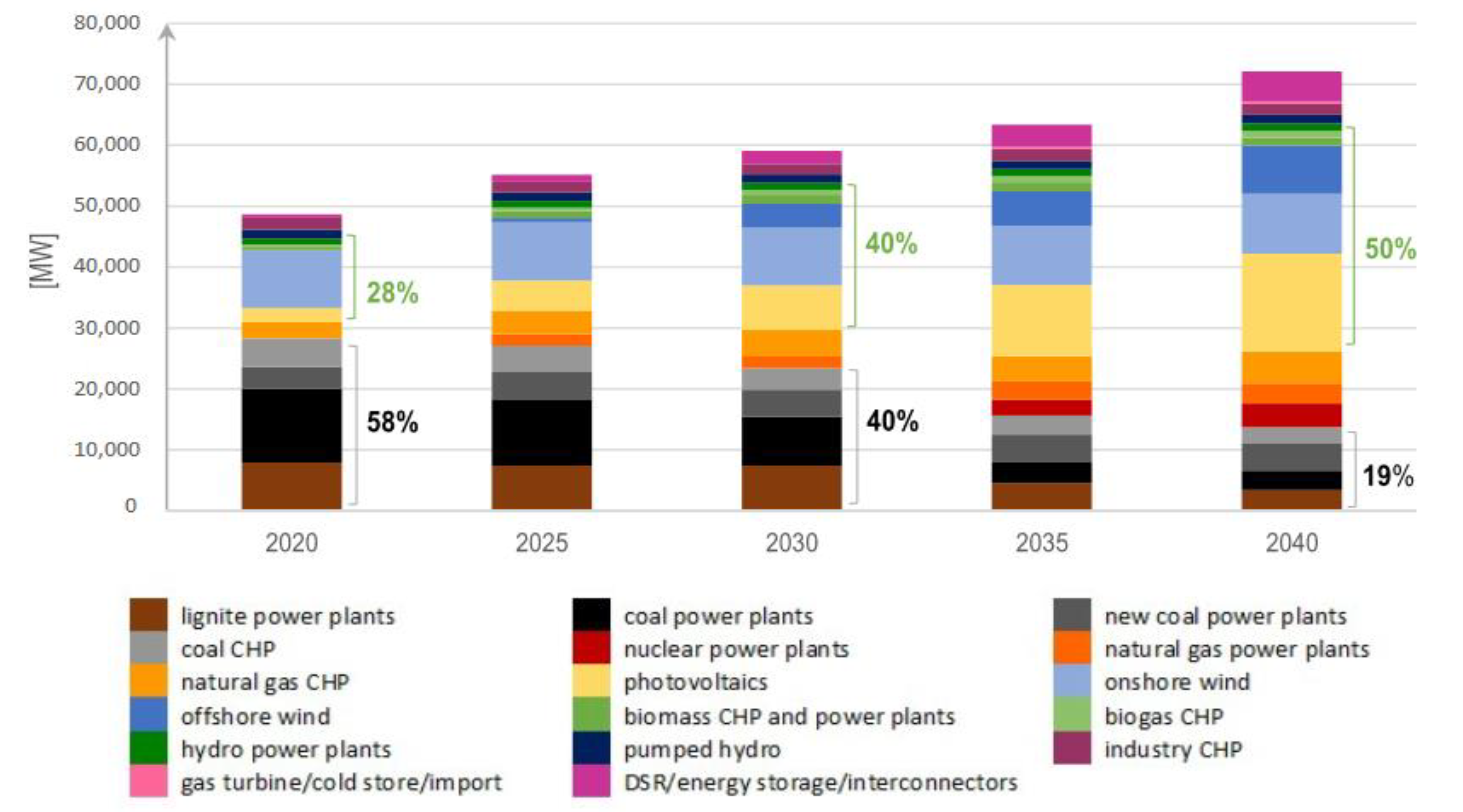
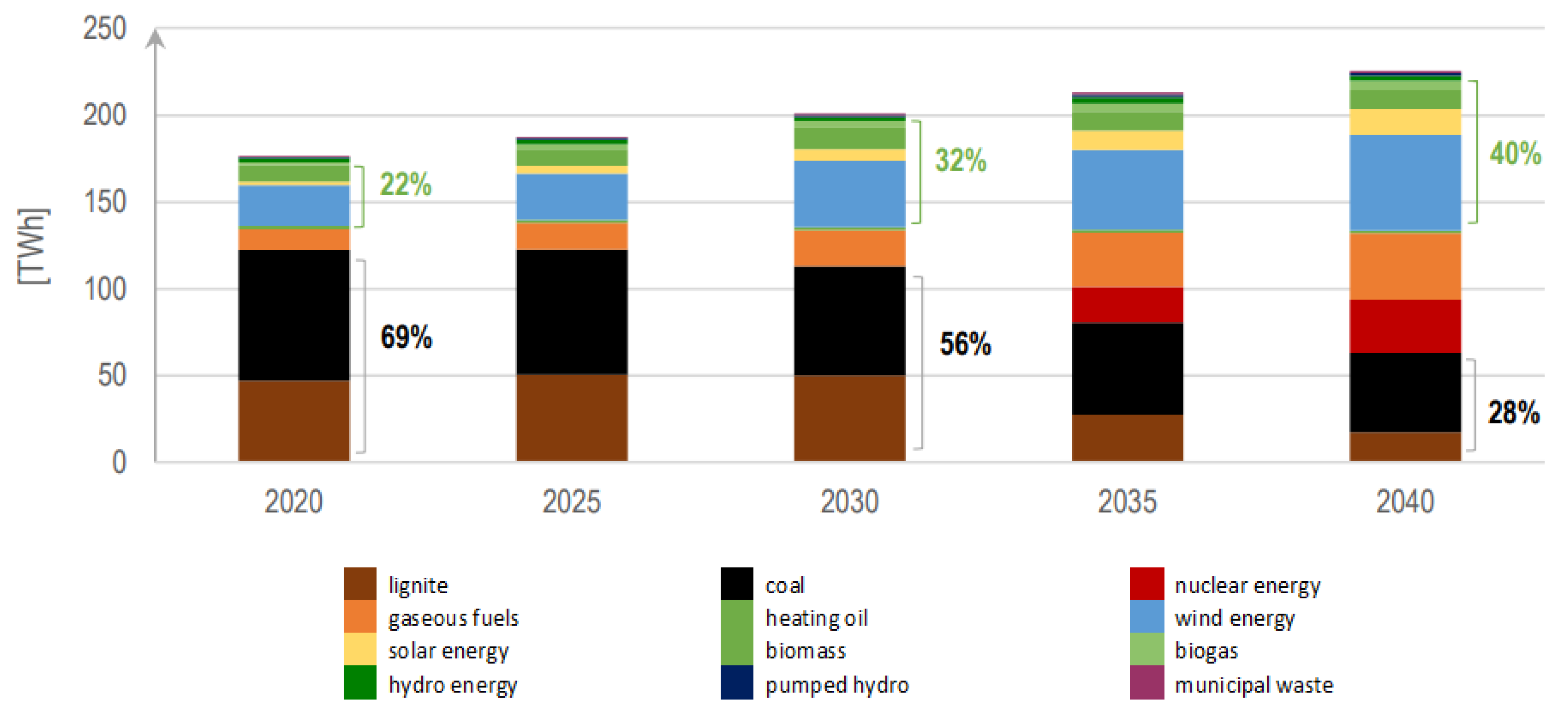
As a result, a set of capacities and production from 2020 to 2040 was obtained. The capacities of the electricity system are presented in
Figure 1. Electricity production depending on the fuel type is shown in
Figure 2. Analyzing the figures, it is observed how a big difference occurs in electricity production from coal when introducing nuclear power energy.
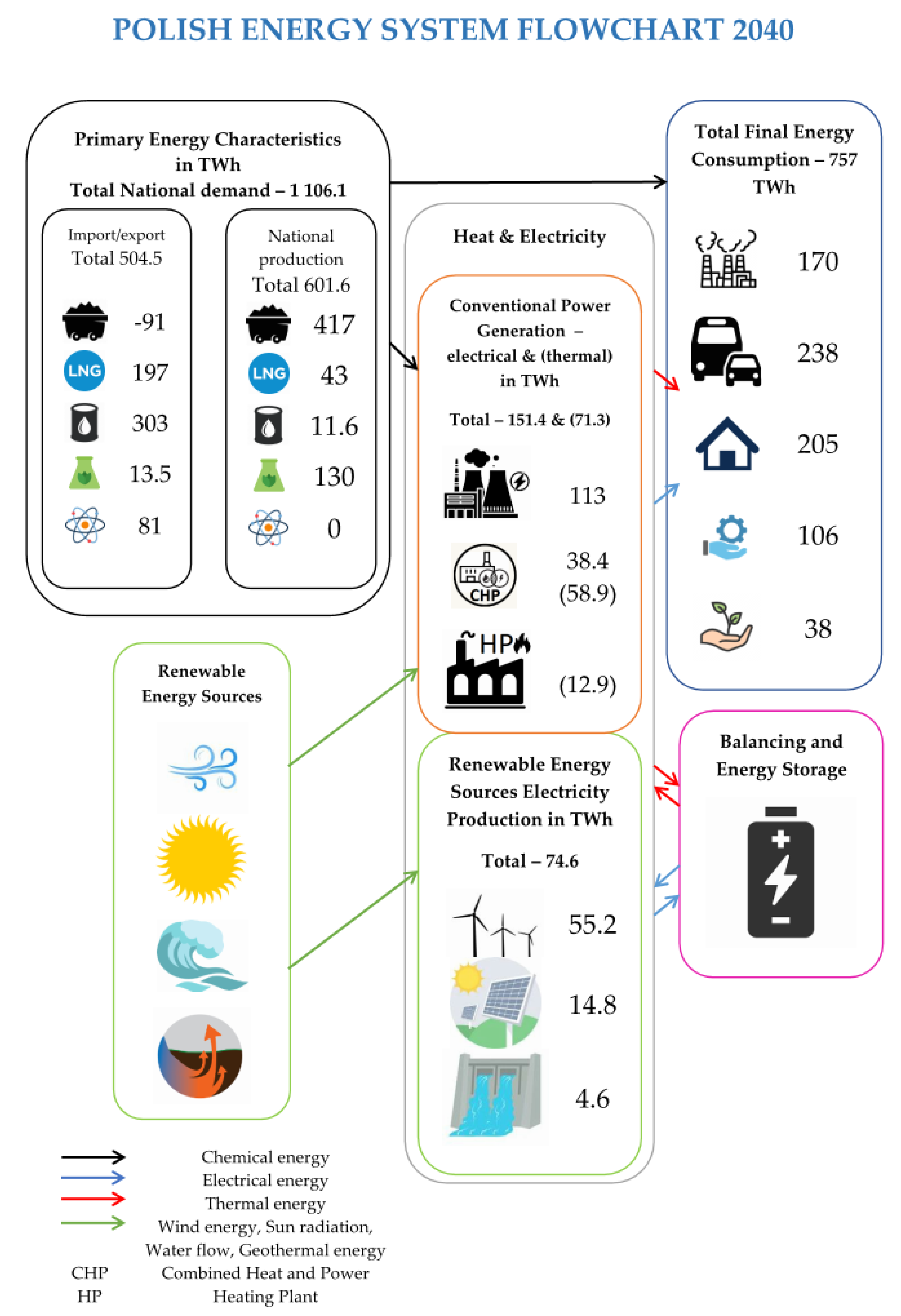
In
Figure 3, Poland’s 2040 energy system is presented, based on the EPP 2040 [
6]. Primary energy includes import/export balance and national production of coal, natural gas, oil, biomass and nuclear fuel. RES are based on wind energy, solar radiation, water flow and geothermal energy (only for heating purposes). Heat and electricity generation is carried out through conventional power units (thermal power plant, CHP and heating plants) and by renewable energy power units (wind generation, photovoltaic (PV) systems and hydropower). The Total Final Energy is presented by consumption the following sectors: industry, transport, households, services, and agriculture. Oil, natural gas, and nuclear fuel are imported in a significant amount (80–100%). Coal is predicted to be the only exportable fuel, i.e., it will mainly be achieved by hard coal and coke. It is forecasted to be the most desirable fuel as well, next to the oil. Transport would be responsible for most of the final energy demand.
An update to the 2014 Polish Nuclear Power Programme was released at the beginning of August 2020 by the National Atomic Energy Agency [
7]. This document proposes and describes four scenarios, and they differ mainly by the year of the assumed nuclear power plants capacities’ implementation. However, two of those scenarios exclude atomic plants from the energy mix. The lowest costs are obtained with 3.3 GW of nuclear power. The main conclusion of [
8] is that the presence of nuclear energy lowers the total costs of energy production. The lowest CO
2 emission in the electro–energy sector was declared with 4.4 GW of nuclear power capacity [
8].
3. Proposed Methodology
As mentioned, the main aim of this work is to evaluate the EPP prognosis by assessing the impact of technology prices on that. To achieve this goal, it is necessary to test all the possible scenarios, evaluating the better solution considering the main goal and the most important constraints of the problem defined by the environmental targets. Two different tools will be used in the present methodology. First, EnergyPLAN will be used to test the different energy mix scenarios. The output of EnergyPLAN will be the global costs and CO2 emissions of the input scenario. Afterwards, an optimizer is necessary to define alternative scenarios allowing the reduction of global costs considering the environment and operation targets.
A suitable environment for modelling the energy scenarios was possible with EnergyPLAN software [
9]. It is developed by the Sustainable Energy Planning Group at Aalborg University, Denmark. EnergyPLAN is described as a user-friendly tool designed in a series of tab sheets [
10]. Programmed in Delphi Pascal, its main purpose is to simulate the national energy systems on an hourly basis, including heat and electricity supplies together with the transport and industry sector. The accessible technology varies from thermal power plants, including nuclear and geothermal with all possible renewable technologies. The software allows the implementation of different energy storage technologies, including pump hydro, compressed air energy storage (CAES), and vehicle-to-grid. The outputs are energy balances and import-export balances, fuel consumption and annual costs [
11]. Other similar tools can be used to perform the present analysis with similar performance. EnergyPLAN was selected because of the past experience of the authors in the use of this tool and its integration with MATtrix LABoratory (MATLAB). This is particularly important to optimize the results that can be obtained by EnergyPLAN.
The software has already been used to analyse the energy mix in different worldwide countries [
12] including several studies from European countries such as Austria, Croatia, Czech Republic, Denmark, Finland, Germany, Hungary, Ireland, Italy, Sweden and, UK. In [
13], the author searched for an alternative energy scenario for 2030 in Colombia. Another example of a holistic analysis was carried out for the Romanian energy system. The aim was to compare scenarios for 2008 and 2013. One scenario is made by the transmission system operator (TSO) of Romania and in the second scenario, nuclear capacity was reduced by 50% [
14]. The Hungarian example includes analysis with two alternative scenarios for the contemporary power system from 2009. This analysis describes issues of the already existing energy system and recommends the implementation of a scenario based on natural gas or biomass [
15]. Benefits of the use of bioenergy, solar thermal and wind energy in a flexible energy system were analysed in Norway with the objective of primary energy consumption reduction [
16]. All those aforementioned analyses show how a country system can be modelled in EnergyPLAN. However, it can be used to analyse single cities energy systems [
17,
18] and for wide systems such as that presented in [
19] for 10 US states or in [
20] for EU 27. Another interesting paper using EnergyPLAN, this time analysing heating sector decarbonisation in Poland, is described in [
21]. These cases show that the software might be used for improvement and validation of already existing projects. A similar purpose is shown in this document.
The use of EnergyPLAN allows a good evaluation of different scenarios. However, other tools are necessary to find the optimal scenario. In the present work, Grey Wolf Optimizer (GWO) [
22] was used to select the best scenario among those tested in EnergyPLAN. In [
22], GWO was compared with other meta-heuristics, such as Particle Swarm Optimization (PSO), Gravitational Search Algorithm (GSA), Differential Evolution (DE), Evolutionary Programming (EP), and Evolution Strategy (ES), showing good results in the presented benchmark. GWO is widely used in power engineering, e.g., the paper [
23] researches the optimal reactive power dispatch with Grey Wolf Optimization and PSO (GWO-PSO). A comparison of GWO with other optimization methods is described during the optimization of micro-grids in terms of energy management and battery-sizing [
24]. Another example is the optimization of the pressured water reactor (PWR) to overcome the issue of in-core fuel management [
25]. An approach to simulate 100% RES production in Portugal in 2050 is described in [
26]. In the present work, the objective of the optimization is to reduce total annual costs under restrictions of CO
2 savings and import and export balance. The goal of present work is not to perform a benchmark of optimization techniques but mainly evaluate the energy mix scenario proposed in EPP 2040. As mentioned, the performance of GWO was already compared with other meta-heuristics showing good results.
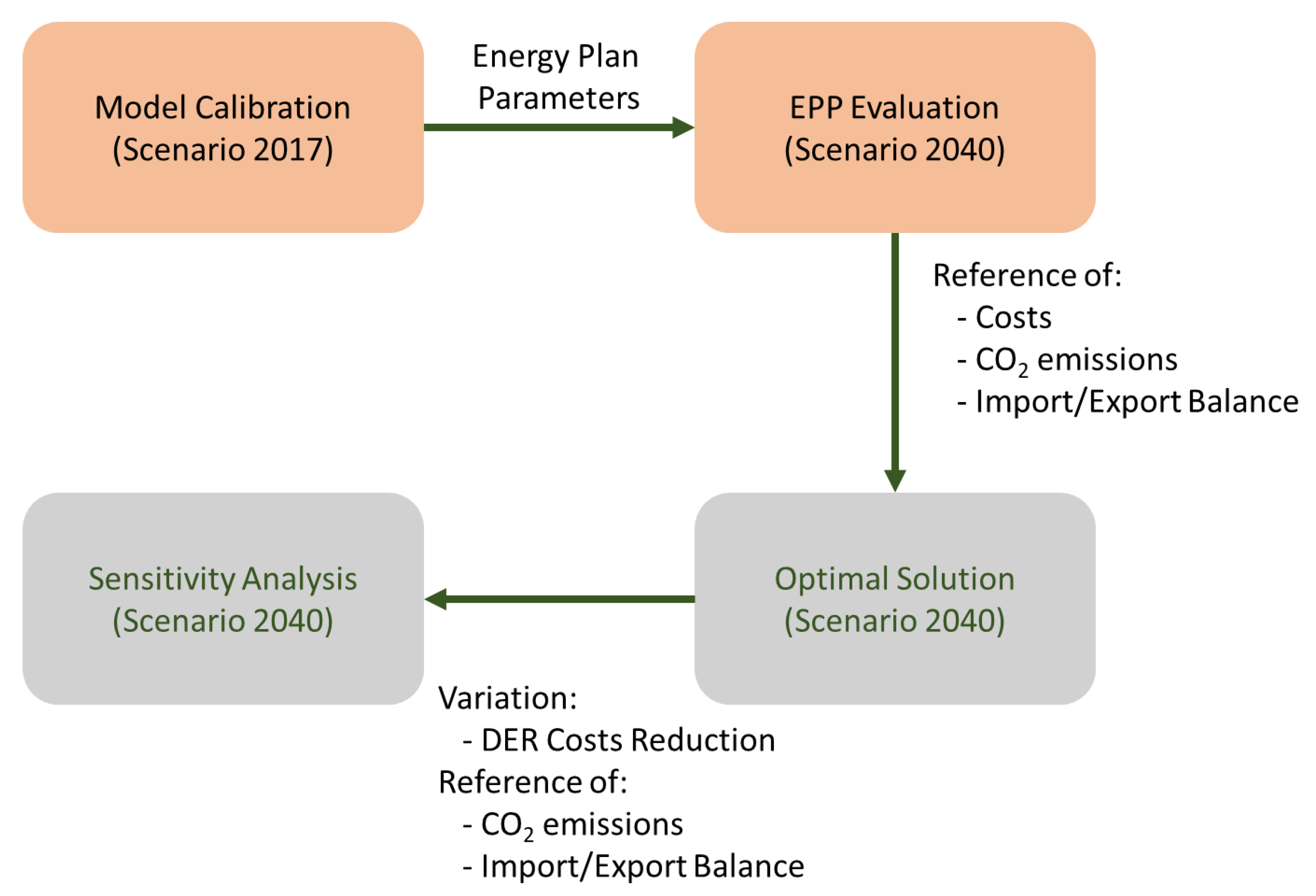
The proposed methodology is divided into four main steps, as shown in
Figure 4. First, it is necessary to calibrate the EnergyPLAN reference model using known values (see
Section 3.1). A reference model helps to better understand the EnergyPLAN software and to find correction factors needed to model the RES. Based on the initial model, it is possible to use the same parameters in a forecasted model. In the present work, this model is the one proposed in EPP 2040 already described. The main goal is to determine the total annual costs, CO
2 emissions, and the import/export balance. These values will be the reference for the optimization model being used for comparison, in the case of total annual costs, and problem constraints in the case of CO
2 emissions and import/export balance. Finally, a sensitivity analysis, considering a variation in the costs (investment and O&M) of distributed energy resources (DER) is performed. This sensitivity analysis also considers the same constraints regarding CO
2 emissions and import/export balance. To perform coherent results, a predefined agent will be implemented into the sensitivity analysis step simulation, containing parameters from the previous simulation.
3.1. Energy Plan Parameters
Concerning the most accessible and actual data, the year 2017 was chosen as a reference year to set up EnergyPLAN variables needed for further analysis. The electricity hourly demand and wind onshore hourly production were taken from Polish Power Grids (Polskie Sieci Energetyczne—PSE S.A.), the Polish transmission system operator (TSO) [
27]. The remaining resources (PV, offshore wind, river hydro etc.) were implemented from EnergyPLAN data for Germany. However, to recreate the Polish conditions, the following capacity factors were assumed: for PV, the capacity factor is equal to 11% [
28]; regarding offshore wind technology, which is not available yet at the Polish system, an insightful study was created by the Warsaw University of Technology [
29] and PKN Orlen [
30] about this technology on the Baltic Sea [
31]. Based on that, the capacity factor of offshore wind was assumed as 46%. All those figures were assumed for the 2017 model as well as 2040.
The modelling intends to balance both heat and electricity demands with an assumption of a minimum 30% grid stabilization share in 2040. Grid stability is a service from TSO to keep up the grid in a stable balance. In EnergyPLAN, this indicator stands for the minimum production provided by the national grid stabilising units (internal thermal power plants and nuclear).
Table 1 presents the major assumptions for the reference and forecast models run in the software. To find relevant capacities several databases were reviewed and selected [
6,
32,
33,
34,
35,
36,
37]. The EPP 2040 proposes 4950 MW of energy storage interconnectors or DSR, in the EnergyPLAN model, it is assumed as CAES capacity entirely. Dammed water supply is manually maintained to obtain proper energy production in this technology.
For the individual heating sources, the household energy utilization data from the year 2017 was used [
42]. For the forecast, coal boilers were replaced by the biomass and natural gas boilers proportionally to keep the same heat demand, whereas heat pumps input was taken directly from EPP 2040 [
6]. Household input is presented in
Table A2. The reason for decreasing the number of coal boilers in households to zero was declared by the local policies of voivodeships’ (administrative units) power (a division of regions in polish administration system) to abandon high emission coal-burning technologies in households [
43]. The main proposition of EPP 2040 for changes in the household heating system is to connect all individual units to the district heating grid. If this is not possible, RES (heat pumps), electric or natural gas technology has to be applied. For solid fuels, the only solution is to obtain a certificate of eco-design or V-class, which makes coal boiler utilization less economic [
44].
Modelling different fossil fuel thermal power plants in EnergyPLAN is relatively complex and limited. To overcome this barrier, in the present work, all the conventional thermal power plants are treated as one technology with proportionally selected efficiency and manually maintained fuel distribution, the same with CHP units. As it is possible to see in
Table 2, the efficiency of the thermal power plants increases from 36.6% in 2017 to 44.01% in 2040 (see the technologies specific efficiencies in
Table A1). This increase is due to the change from coal thermal plants to gas turbine combined cycle (GTCC). Assumptions regarding fuel distribution and efficiencies are presented in
Table A3 and
Table 2.
In EnergyPLAN, costs are divided into investments, fuel, operation and maintenance, and external electricity market costs. The model summarises the input capacity specifications for the production units, and one can add unit prices, lifetimes and fixed operation and maintenance costs. The interest rate must be defined for the calculation.
Concerning the investment, O&M, fuel and fuel-handling costs, several data are available in the literature. To make this work coherent and transparent, all data were taken from an EnergyPLAN database of costs [
48]. The costs values for the year 2040 are presented in
Table A4,
Table A5 and
Table A6.
The assumption of import/export balance at the level of 0 was decided based on EPP 2040 forecast condition, where this balance was also assumed as zero. This assumption is considered as a constraint in the optimization problem. To evaluate this balance, all the interconnection capacities are considered in the EnergyPLAN and taken into account in the simulations. Specific data of the European Commission on taxes and EnergyPLAN database were used as assumptions (see
Table A5) [
48,
49,
50]. Variable costs illustrated in
Table A6 were taken from EnergyPLAN database [
48]. The assumed interest rate was 3% and CO
2 emission cost was 40.6 (EUR/t CO
2). All prices are discounted to euro value from 2009 [
48].
3.2. Optimization Process Definition
To evaluate the proposed solution to 2040 and to find alternative solutions considering the costs uncertainties, a metaheuristic method named Grey Wolf Optimization (GWO) was used. Similarly to the pack group, the leaders are named Alpha (α), then next ranked are Betas (
β), further Deltas (
δ) and the lowest-ranked wolves are Omega (
Ω) [
22]. In this method, solutions are presented with the same hierarchy. The theory stands that those three wolves are the closest to the prey and their positions are used as an input for the next iteration. However, the last ones, Omega, update their position according to the Alpha, Beta and Delta. This behaviour allows the probability of finding local extreme to significantly decrease.
The distances from
α,
β and
δ wolves stand for
,
and
to each of the remaining wolf
are calculated using Equation (1) applying which the response of
α,
β and
δ wolves on the prey viz.
,
and
can be determined as represented in Equation (2).
The variables of controlling parameters of the algorithm which are
a,
and
are calculated using Equation (3). Random vectors
and
are in the range of [0, 1]. These vectors allow wolves to reach any point between the prey and the wolf. Vector
allows to control the activity of the GWO algorithm and is used to determine
. The component values of
vector decreases linearly from 2 to 0 over the sources of iterations.
provides help in including some extra weigh on the prey to make it harder to be found by wolves. Lastly, all other wolves update their positions
using Equation (4) [
51].
To run the optimization, a specific code in MATLAB add-on to the EnergyPLAN was customized. A similar approach was already used to create scenarios allowing 100% renewable energy mix forecast in Portugal 2050 on the mainland [
52]. In
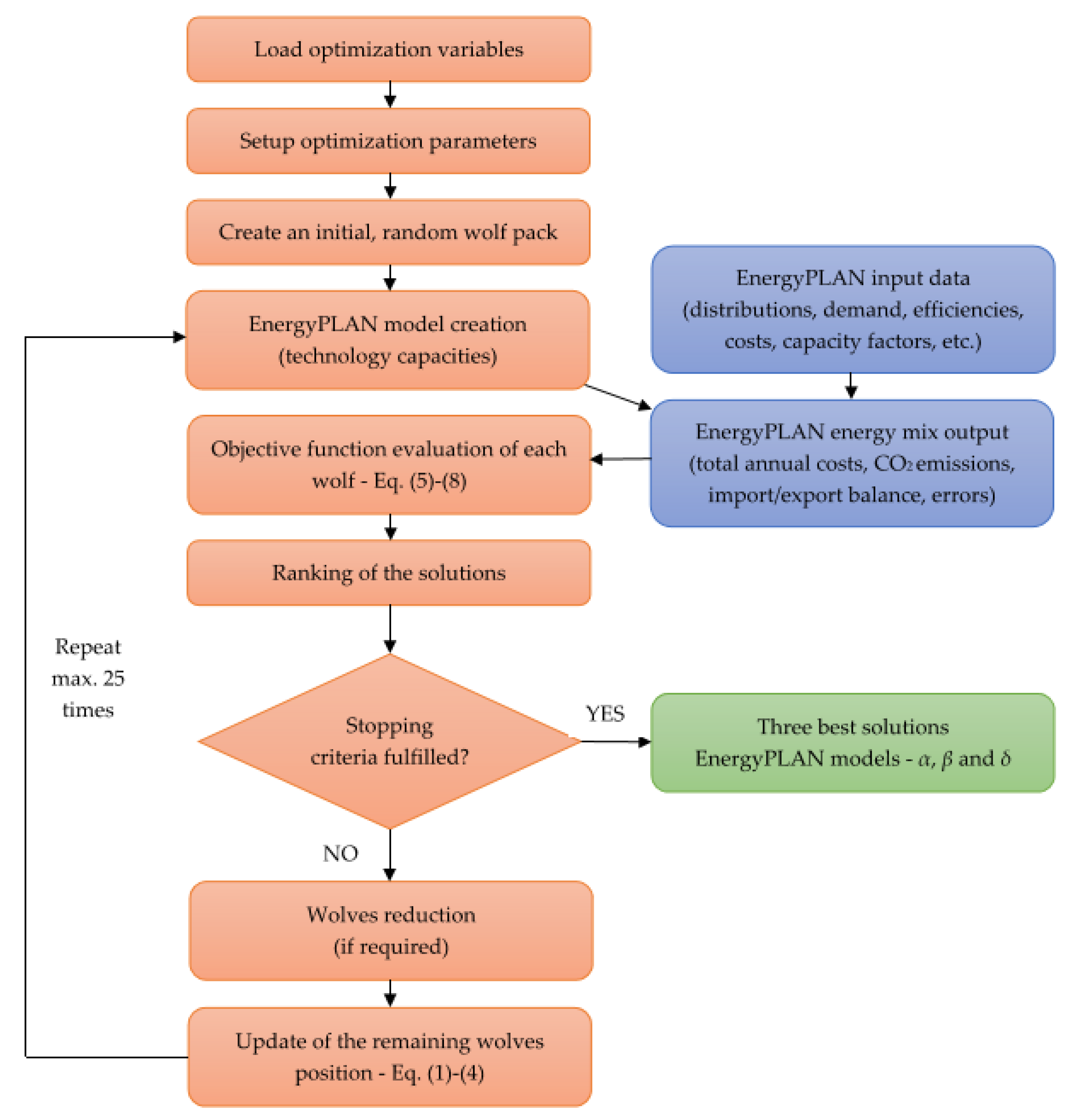
Figure 5, it is illustrated how the optimization process with the EnergyPLAN software will be carried out. The process starts with a verification of the destination of the files and loading a file with capacity limits and variables description (technologies). The next step is setting up the optimization parameters (number of runs, stopping criteria, number of agents). Creation of a random set of agents (wolf pack) is initiated after setting up the optimization, then each individual agent (wolf) is processed in EnergyPLAN resulting in a set of models. Every model is a complete energy mix scenario. To carry out this operation, input data concerning distributions, demand, capacity factors, efficiencies and costs are necessary. All those parameters are assumed the same as in the EPP 2040 model. The next step is the evaluation of the objective performance, minimizing the fitness function Equations (5)–(7). The objective is to minimize total annual costs with restrictions for CO
2 emission and import/export balance limitation, the evaluation process is already described further on. The lower the value of the total annual costs, the closer to the ideal energy mix (prey), thus a ranking of solutions is created in the next step. Optimization ends after 25 runs, or after reaching the stopping criteria. i.e., if the change in the costs is lower than 5 million euros within 5 consecutive runs, the optimization ends by saving three best solutions—
α,
β and
δ. If the criterion is not fulfilled, another condition might reduce the number of agents and create a new wolf pack relaying on the previous solutions. Agents decrease by 100 every 5 runs, although, 50 agents is the lower limit. Prey approach and the wolf destination update is expressed by Equations (1)–(4). New capacities (wolf locations) are now evaluated again in the step “EnergyPLAN model creation” until the stopping criterion is not fulfilled.
EnergyPLAN inputs are identical as those used in EPP 2040 model, thus the parameters are constant through the process. The variables representing the capacities of technologies and energy storage parameters are changed in every agent evaluation. The output used in the optimization are the total annual costs, CO
2 emissions, import/export balance and errors. The software may include 5 types of error characterizing invalidation of the energy model. To fully understand EnergyPLAN methodology, an exhaustive 15th version of the manual can be found in the document [
53].
In this work the objective is to minimize total annual costs (TAC − a sum of CAPEX + OPEX for each technology
Tech, see Equation (6)), considering that the total CO
2 emissions (
) should be lower or equal in comparison to the EPP 2040 forecast scenario (
) and the import/export balance should be close to 0 during a year. Therefore, penalty functions were implemented. Equation (7) stands for the CO
2 emission performance, predefined
indicates whether the obtained value of
is lower than the reference one. The penalisation only occurs if the optimized solution implies a CO
2 emission higher than
. Another penalisation (see Equation (8)) takes place while exciding 0.1% of the total electricity demand by import/export balance. The added value to the objective function mathematically described in Equation (8). The fitness function is described by the Equation (5), as a ratio of the total annual costs Equation (6) and penalisation functions Equations (7)–(8). If the model is technically invalid, the
is added to the penalisation equation.
The modelled variables were capacities of wind onshore and offshore, PV, river hydro, dammed hydro, nuclear and conventional power plants. To balance electricity generation and consumption, pumped hydro and CAES technologies were used. The forecasts include electricity and heat sector, however, only the electricity sector was optimized.
The limits were assumed to be due to the potential of technologies or according to the highest found value in different forecast documents [
6,
8] (see
Table 3). All minimum capacities, except thermal power plants, are taken from the year 2017. Thermal power plants have a minimum assumed to be the CHP capacity in the 2040 EPP forecast. PV has its maximum set as a capacity in EPP 2040, wind onshore and river hydro, dammed hydro as International Renewable Energy Association (IRENA) potential [
54]. Wind offshore and nuclear maximum capacities were taken from the existing scenario in the atomic agency report [
8] and thermal power plants have an arbitrary maximum.
4. Results
In this section all verification values are presented for the reference model and forecast reconstruction model, then the results of the optimization and its sensitivity analysis are compared.
Firstly, in
Section 4.1 for the reference model electricity demand, production, export and import balance are compared. Next, comparison is of all electricity and heat production units. Then, the primary energy utilized in electric and heating sector is verified. To verify the EPP 2040 forecast comparison of its electricity and heat production, demand, export and import was carried out in
Section 4.2. The results obtained using the proposed methodology based on GWO are compared to the EPP 2040 forecast scenario (modelled in EnergyPLAN and presented in
Section 4.3). A sensitivity analysis is illustrated as a comparison of total annual costs in
Section 4.4.
4.1. Reference Model (2017)
Firstly, the reference model was calibrated according to the production and primary energy utilization, considering real values. The error lower than 5% was assumed as a limit for the model validation.
In
Table 4 the balance of demand, production and interconnection exchange is demonstrated.
Table 5 and
Table 6 present electricity and heat production. Specific data from Polish administrative entities were used to verify the model [
32,
36,
42].
Verification of primary energy utilized is shown in
Table A7,
Table A8 and
Table A9. Similarly to the production and demand, specific data were used for the validity of the model [
36,
37,
38,
55]. The software allows to include only four types of fuel, i.e., in section “biofuels” municipal waste and other alternative fuels were assigned. In this project, they are named biofuels and alternatives.
4.2. Polish Energy Policy 2040 Scenario (EPP 2040)
A similar procedure was applied to the forecast, validity was confirmed by the difference between the values presented in the Polish Energy Policy 2040 forecast [
6] and EnergyPLAN model. The main results are presented in
Table A10,
Table A11 and
Table A12.
The value of total annual costs is equal to 30,943 million euros and CO2 corrected emissions are 91.492 million tonnes CO2. Corrected emissions stand for the emission produced by the internal system including import/export balance emission produced by the external sources. This value diverges from the internal system emissions only in the case of modelling the reference year 2017 and EPP 2040 forecast, and the GWO model has those emissions as coherent. Also, the import/export balance is not exactly 0. An explanation can be given by the use of the same parameters of 2017. The parameters used in EPP 2040 report are not known. Nevertheless, the obtained import/export balance is less than 1% of total demand.
4.3. Optimization Results
In the present section, the results obtained considering the methodology proposed in
Section 3.2 are presented. The boundaries of CO
2 emissions and energy import/export balance are the values obtained in the previous analysis (
Section 4.2) that are 91.492 million tonnes CO
2 and 1.83 TWh, respectively. The comparison of the EPP 2040 scenario and the results obtained by GWO are presented in
Table 7.
Comparing the two scenarios (see
Table 7), it is possible to observe that the wind technologies experienced the highest capacity growth. Offshore wind achieved its maximum capacity limit. Also, the production in river hydro increased significantly (22.08%). This is very important for compensating the imbalances created by the technologies based in renewables. In contrary, PV technology is the least supported technology and its variation to the EPP scenario is the largest. This can be explained by the investment costs associated with this technology as well as the low capacitor factor. It is important to mention that the increase in PV use will result in a higher demand for storage capacity.
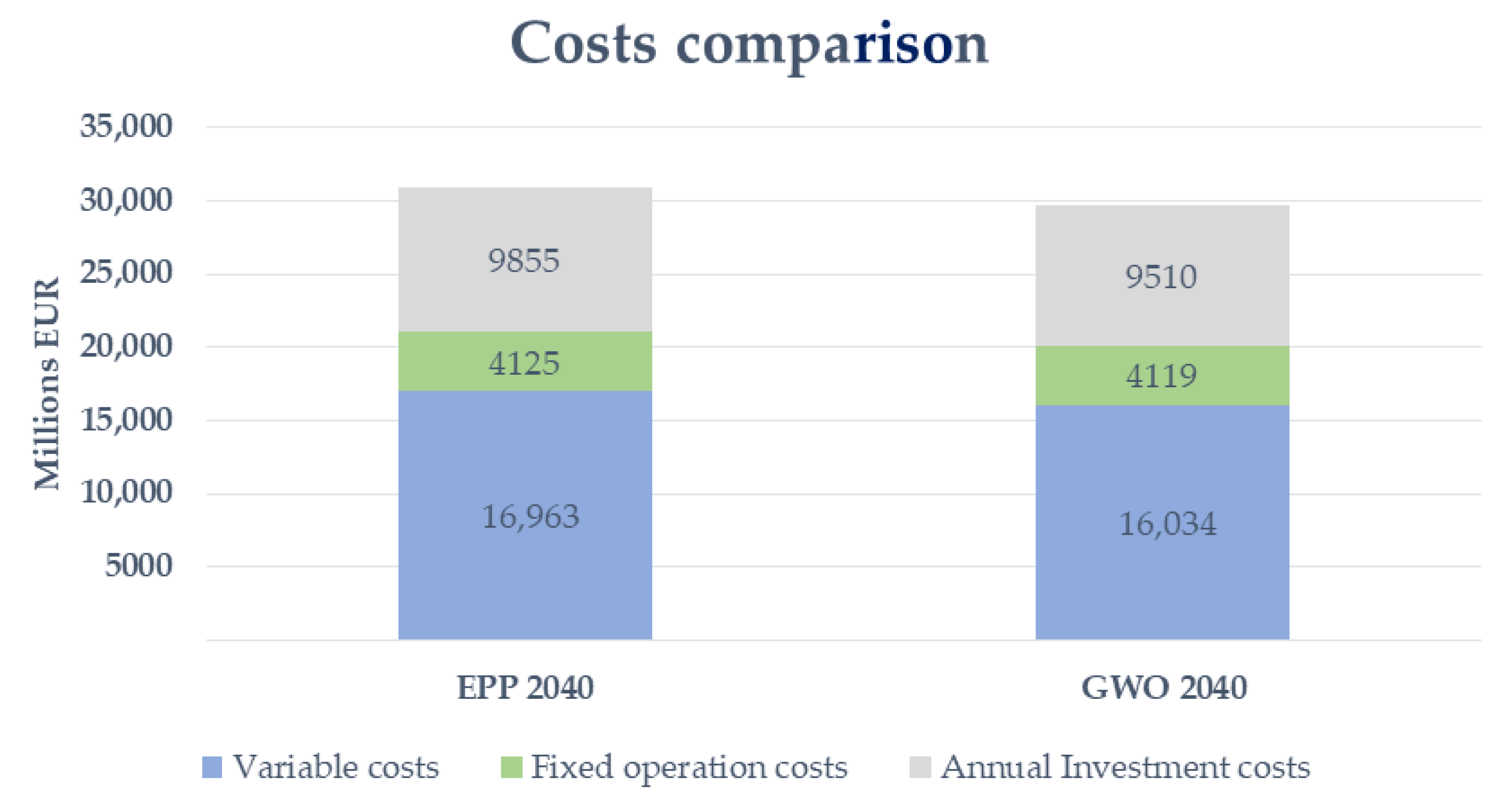
The optimization produced over 4% costs savings with CO
2 emission reduction for almost 9% (see
Table 8). Share of RES in electricity production fulfils the EPP conditions. The costs described are detailed in
Figure 6. Operational costs stay at the same level, whereas variable and investment costs decrease.
4.4. Sensitivity Analysis
Sensitivity analyses considering RES costs reduction (
Section 4.4.1), carbon tax or CO
2 emission cost variation (
Section 4.4.2) and natural gas price rise were performed successfully (
Section 4.4.3). Resulting in costs, CO
2 emission, electricity production and capacity graphical interpretation. RES technology is becoming more accessible and its cost decrease [
56]. It is estimated that from 2009, PV module prices declined by 90%, and wind turbines from 2010 experienced a fall by 55–60% [
57]. If this trend will be kept at a similar level, those technologies will become even more competitive, thus, a sensitivity analysis was carried out (see
Table A13 for the RES sensitivity analysis input). The European Commission sets up a cap for the CO
2 emission in the European Union (EU), therefore each tonne of CO
2 has a price [
58]. Producers trade allowances to emit CO
2 in order to reduce the variable costs of their units. The price depends strongly on the current policies e.g., European Green Deal, thus a sensitivity analysis concerning 30% variety of this cost was performed [
59] (see
Table A14). Additionally, an analysis of the natural gas price was carried out, due to the uncertainties in fossil fuel-based resources until 2040 [
60,
61]. It forecasted that European natural gas demand will vary from nearly 250 to more than 500 bcm (billion cubic meters) in 2040, based on a holistic study from the Centre for European Policy Studies (CEPS) [
62]. This report reviews recent studies regarding the future of natural gas. Together with natural gas price variation between 30.7 and 47.5 EUR/MWh within 2030 and 2050, according to the IEA [
63] data enclosed in the heat roadmap for Europe [
20], this was the reason for sensitivity analysis of natural gas prices. The input of this analysis is presented in
Table A15.
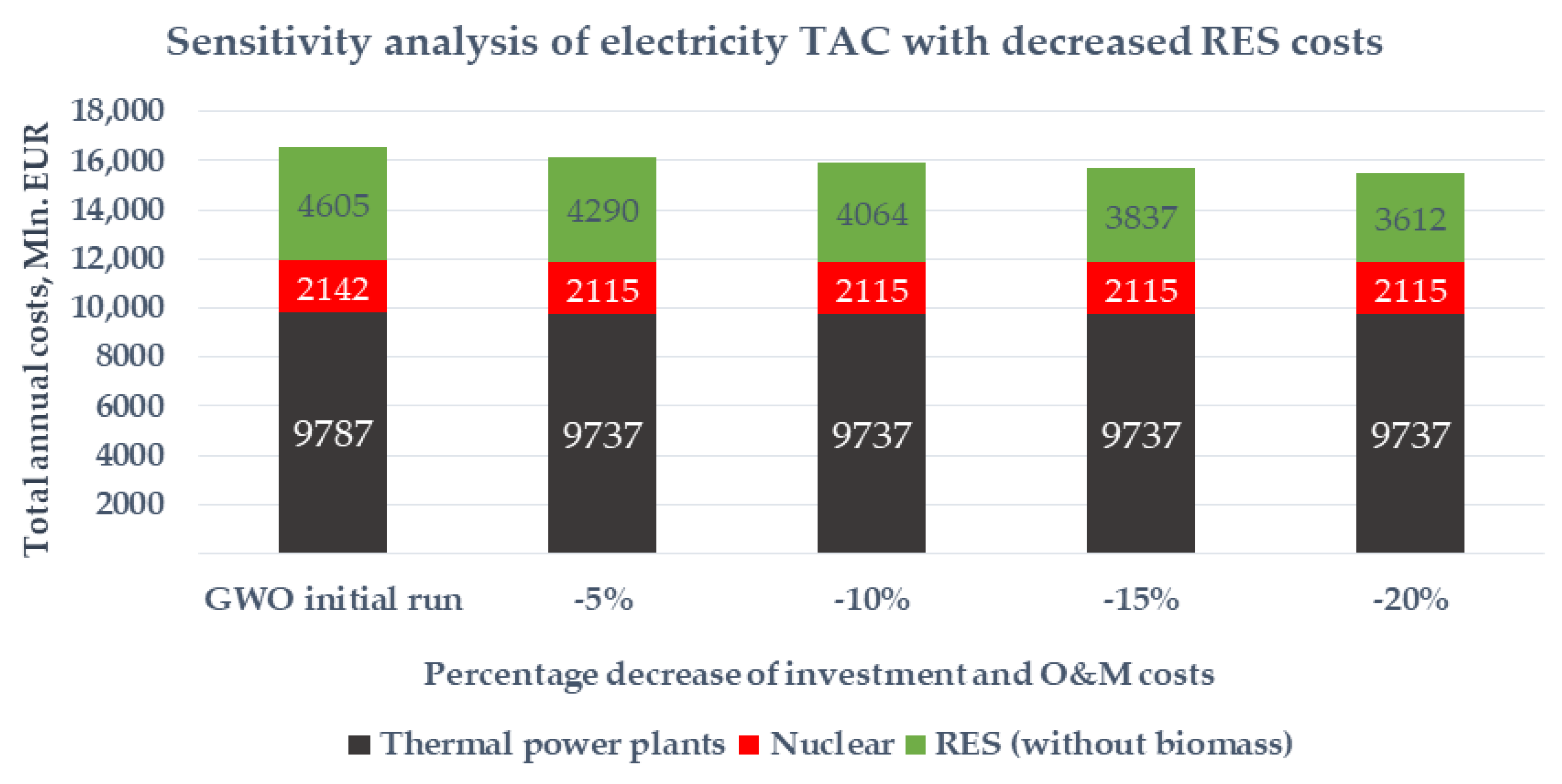
4.4.1. Sensitivity Analysis—Renewable Energy Sources (RES) Fixed Costs Decrease
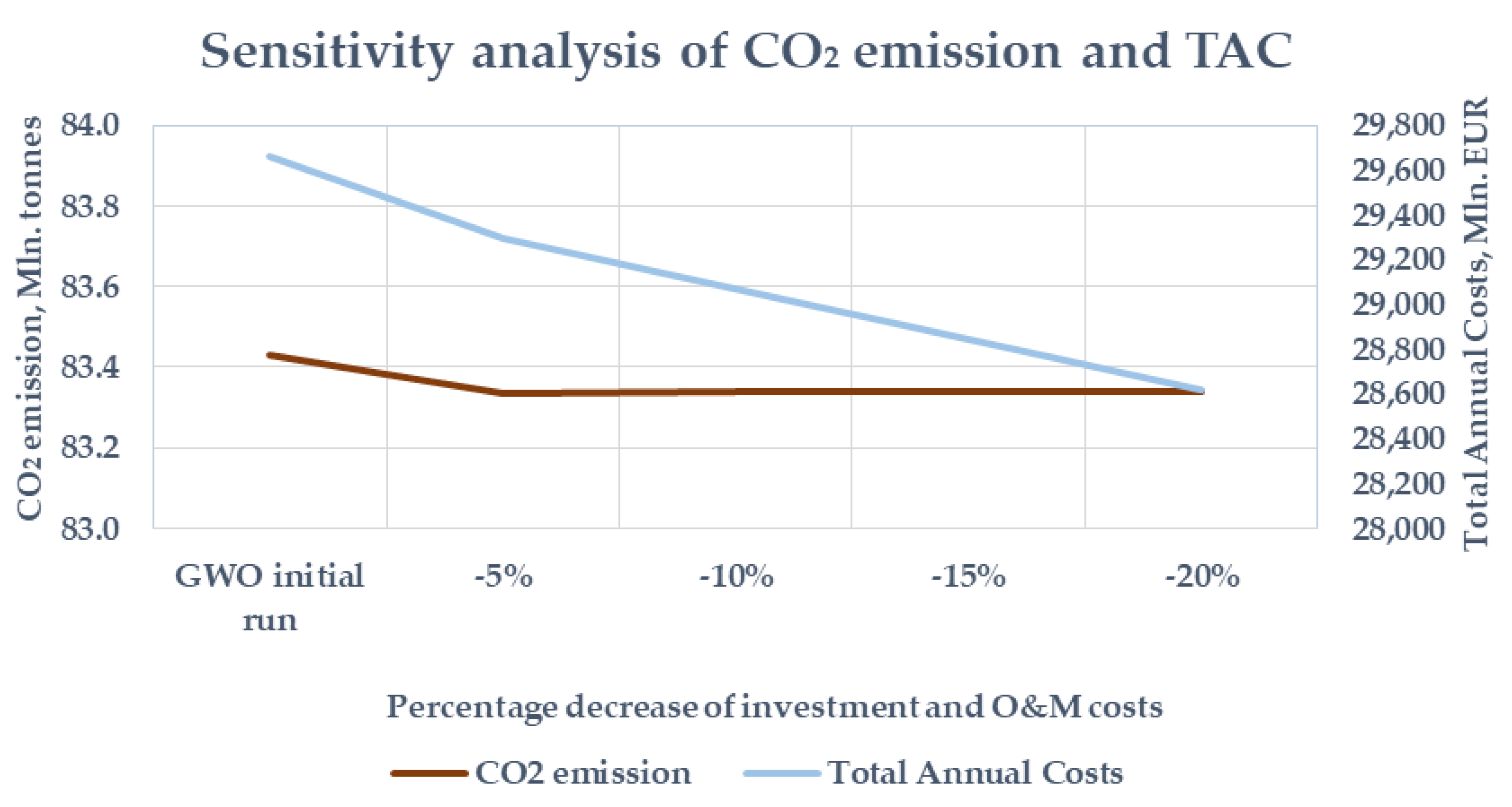
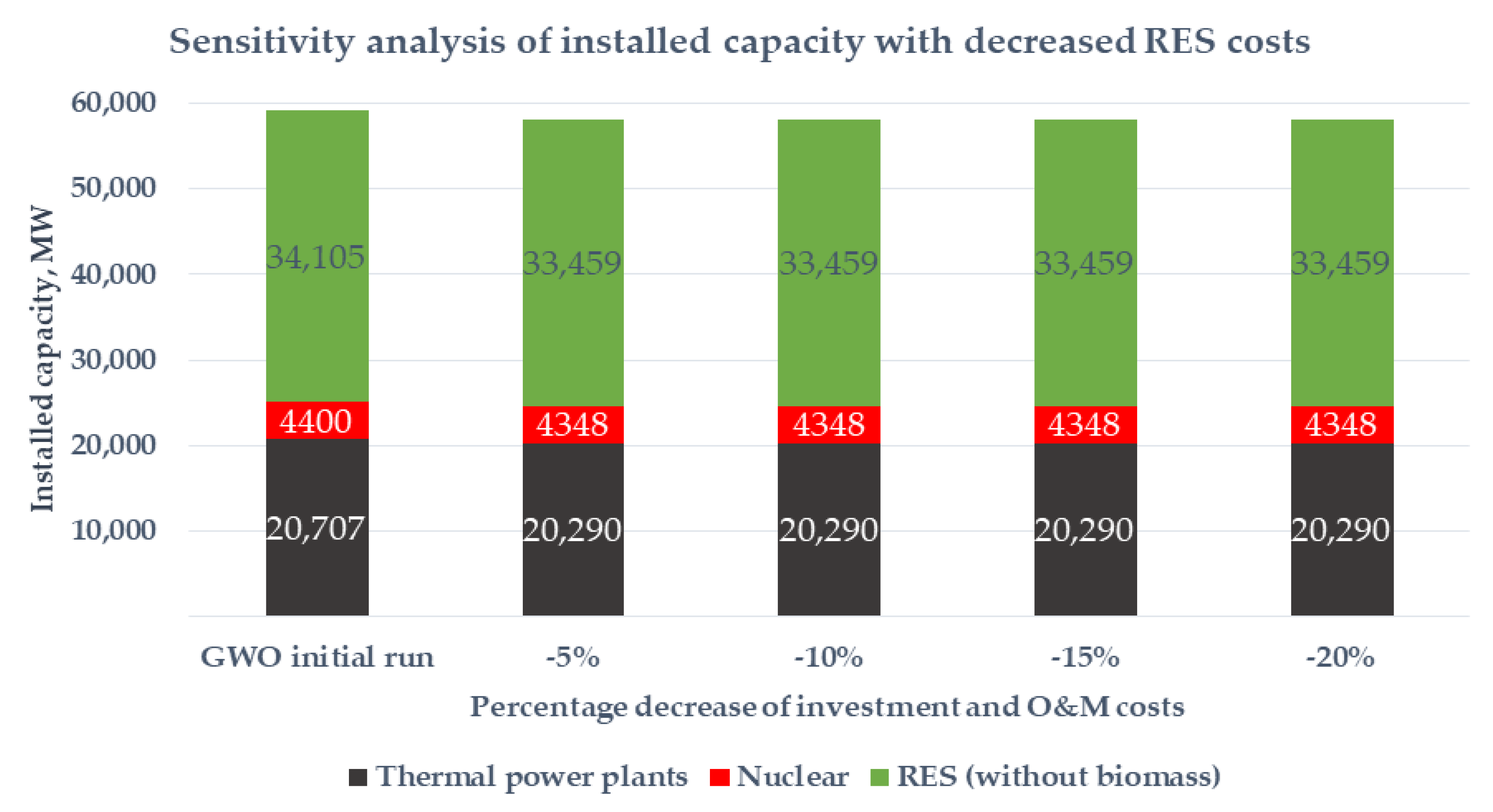
Investment, operation, and maintenance costs were decreased by 5–20% with a step of 5% in the RES analysis. The main results are presented in
Figure 7. As expected, the global investment decreases, and the savings are around 1.046 billion euros a year which represents 3.53% when compared with the initial scenario. Considering the obtained values, it is possible to conclude that decreasing costs of RES did not bring any significant changes in the energy mix (see
Figure 8 and
Figure 9) and CO
2 emissions (about 0.1% variation), while the electricity total annual costs (
Figure 8) decreased slightly (6.59%). Considering the electricity sector, the total annual costs of RES in this sector decreased by about 21.56%.
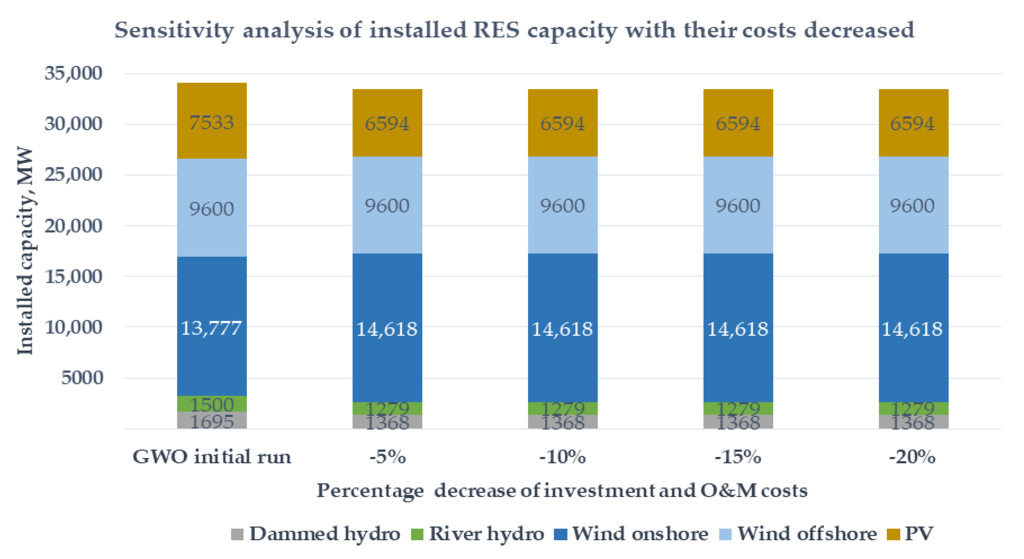
The only change that occurred during the analysis is a small reduction in the capacity of coal and nuclear power plants (
Figure 9) and mainly the reduction of almost 1 GW in the PV fulfilled by the onshore growth, 841 MW (see
Figure 10), and a very small decrease in the nuclear energy. This can be explained by the lower capacity factor of PV in Poland (around 11%).
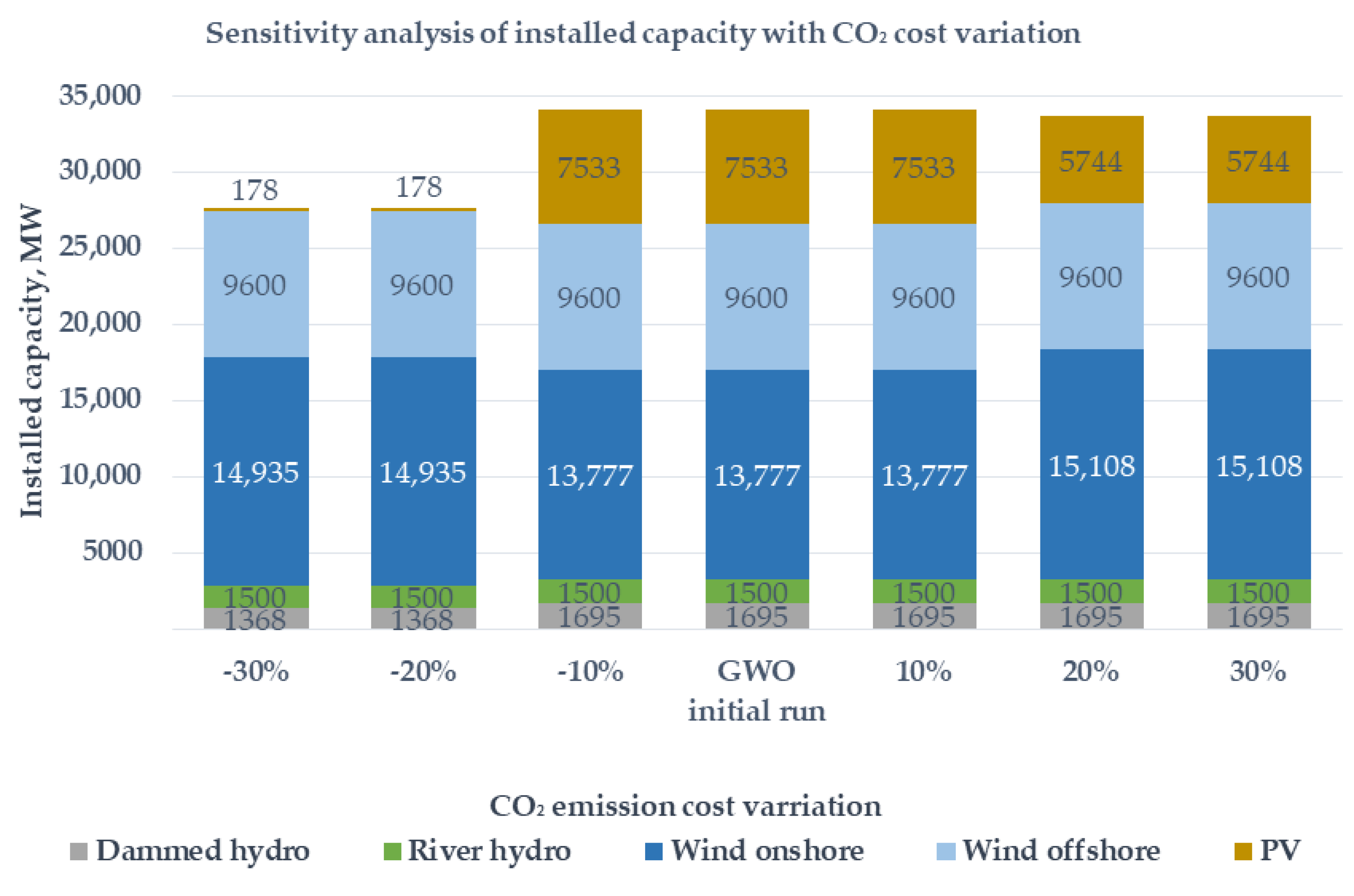
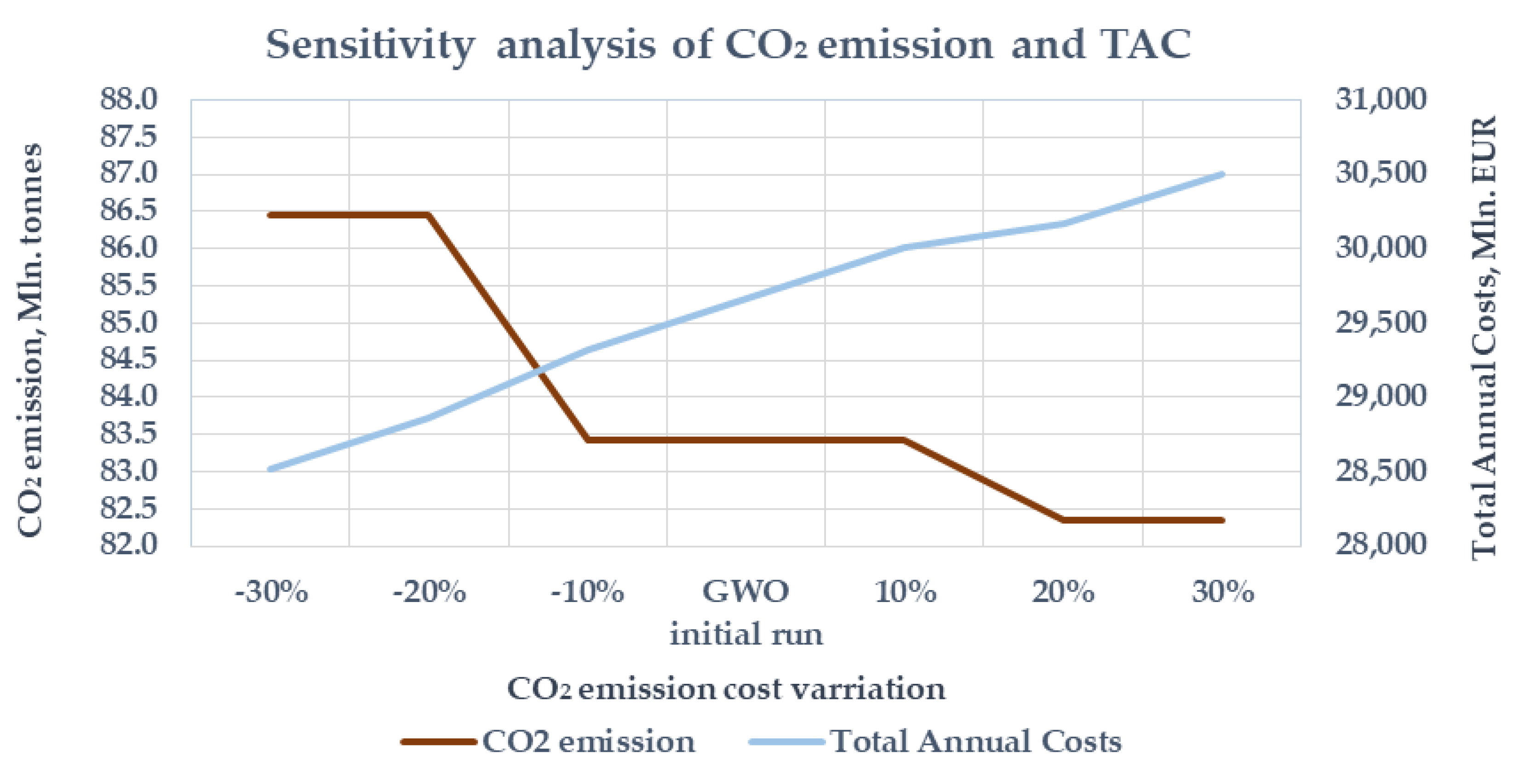
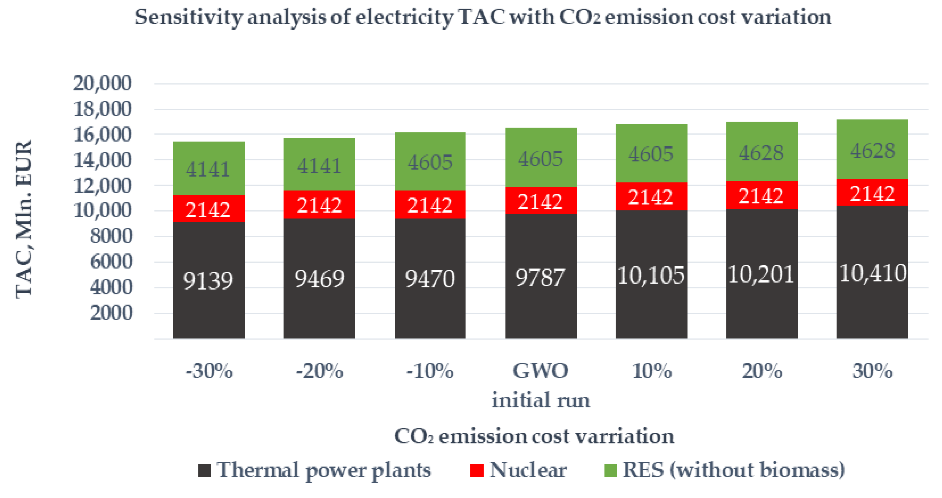
4.4.2. Sensitivity Analysis—Carbon Tax Variation
To evaluate the impact of CO
2 emission cost on the energy mix, six simulations were performed from a 30% decrease of gas cost to a 30% increase, with a 10% step. The CO
2 emission and TAC as well as electricity TAC are expressed in
Figure 11 and
Figure 12. Tax decrease resulted in predicted electricity TAC reduction for about 1112 million euros (6.73%), on the other hand, carbon tax increase determined electricity TAC rise for about 645 million euros (3.9%). The CO
2 emission reached 3.02 million tonnes increase (3.62%) and 1.092 decrease (1.31%), respectively. The marginal cost of thermal power plants was equal to 68 EUR/MWh in 30% tax decrease and raised for approximately 3 EUR/MWh in each step (per 10%) to be equal to 85 EUR/MWh in a 30% carbon tax increase.
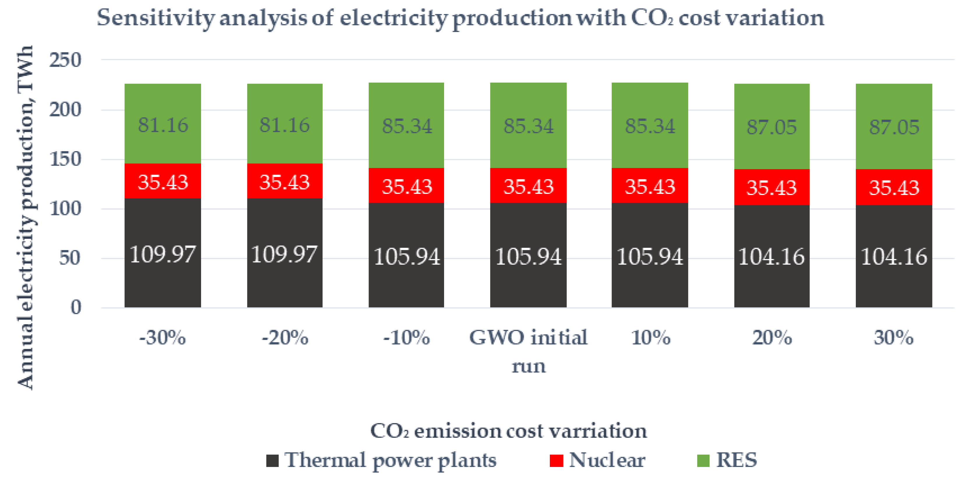
The energy mix changed drastically in RES technologies. Carbon tax decline implied higher fossil fuel electricity production, reducing PV capacity to nearly zero value (
Figure 13 and
Figure 14). Within 10% cost oscillation, the energy mix remained the same as the initial one. However, 20% and 30% increases of the tax indicate very high onshore capacity, 15.108 GW, and lowers the PV for almost 1.8 GW. River hydro experienced constant capacity during the whole analysis.
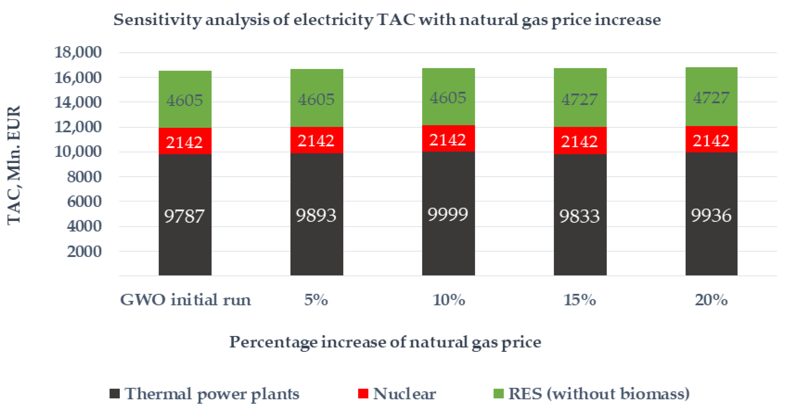
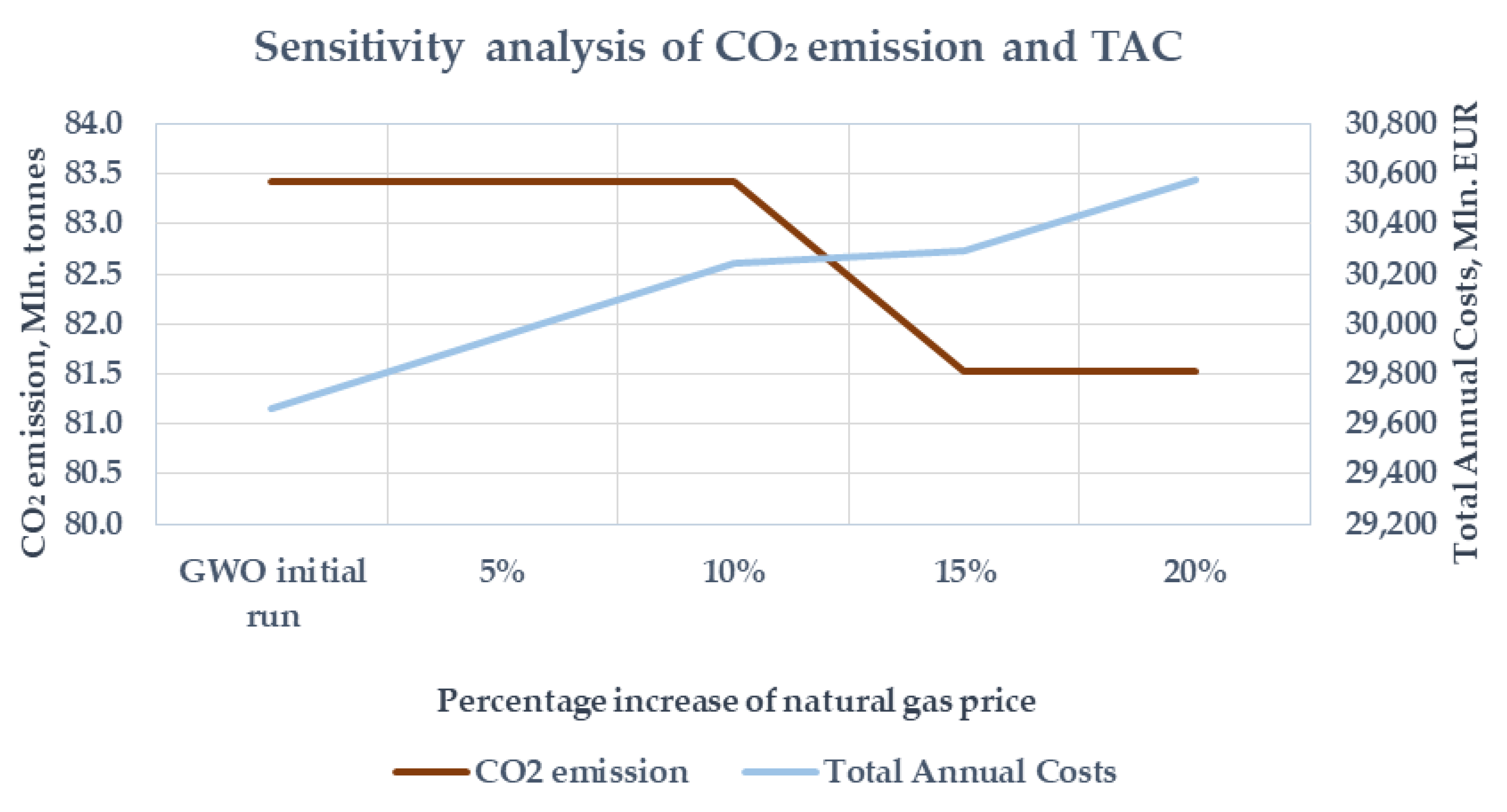
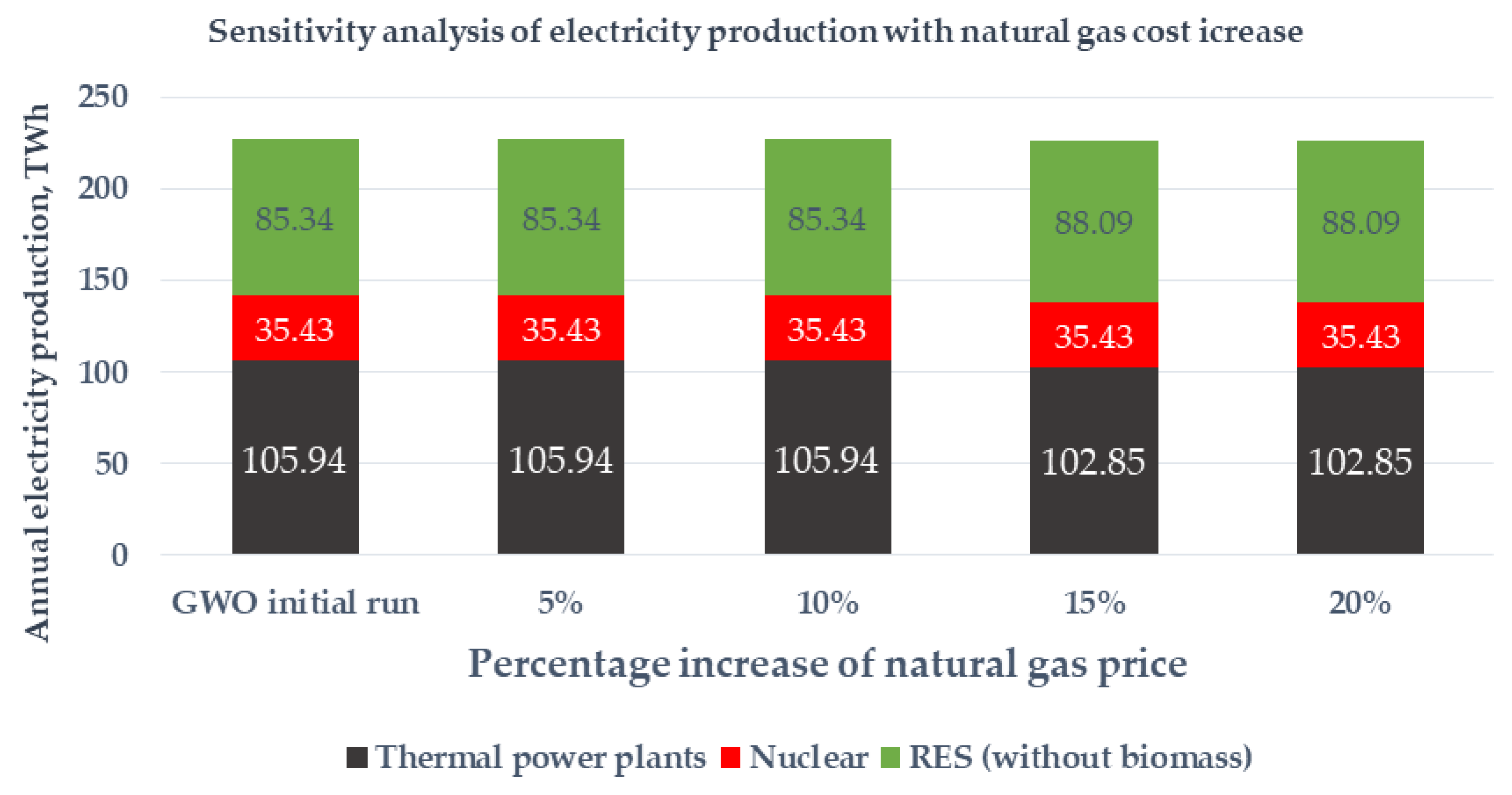
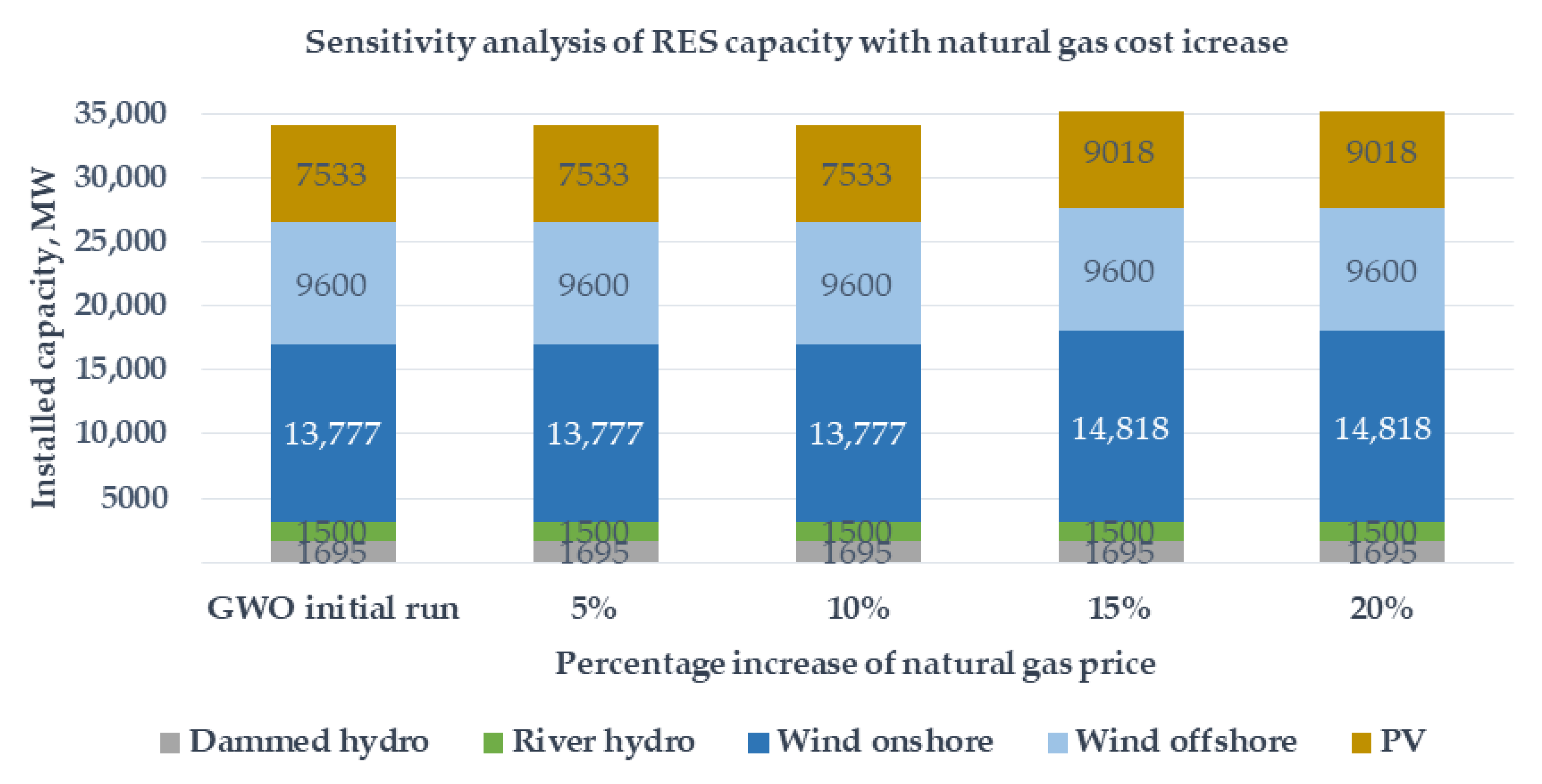
4.4.3. Sensitivity Analysis—Natural Gas Price Increase
To determine the natural gas sensitivity, four simulations were carried out increasing the cost of this fuel. The natural gas price was increased by 20%, with 5% step. The CO
2 emission and TAC are illustrated in
Figure 15. TAC increased by about 914 million euros (3.08%), whereas, CO
2 emission decreased for about 1.9 million tonnes (2.28%). Electricity TAC increased just for about 270 million euros (1.64%), which can be explained by the RES replacement (see
Figure 16 and
Figure 17). The marginal cost of thermal power plants production increased from 77 to 81 EUR/MWh.
The main energy mix changes include PV increase for almost 1.5 GW and wind onshore for over 1 GW within 15% and 20% of the natural gas rise (see
Figure 18). River hydro and dammed hydro remained at a constant level during this analysis.
5. Conclusions and Discussion
This paper presents an alternative scenario for the energy mix in Poland in 2040. The proposed scenario was obtained using an optimization process based on Grey Wolf Optimizer (GWO). Compared with the official energy mix scenario proposed in EPP 2040 [
6], it is possible to conclude that the proposed solution allows a total annual cost reduction of 1.3 billion euros (over 4%) with respect to, with some minor differences, the total CO
2 emissions and the import/export balance. From the results, it is possible to verify that the CO
2 emissions are lower in the proposed method (less than 9%) and the import/export balance are the same.
The savings have been obtained mainly through the use of more offshore wind power capacity, and by the use of more river hydro generation. Other important difference, comparing the obtained scenario with that of the EPP 2040, is the reduction of PV capacity from 16 GW to 7.53 GW. This can be explained by the costs associated with this technology and the lower capacity factor in Poland. The nuclear power capacity is similar in both reports.
A sensitivity analysis, considering the reduction of investment cost in renewable base technologies are also presented showing a reduction of the total annual costs. The overall conclusion is that no significant changes in the energy mix appear if those costs decline. The analysis projected carbon tax sensitivity and natural gas increase as well, resulting in a higher contribution of the carbon tax in the variable costs than natural gas. Carbon tax reduction resulted in a complete decrease in PV electricity production, except for this occurrence, and no significant changes in energy mix were recorded during the analysis.
Future work is expected to compare the performance of GWO with other heuristics to this specific problem and the improvement of the existing methodology using an optimized initial solution. Another aspect that should be addressed in future work are the costs associated with the transmission grid development. In the proposed solution, huge capacities of wind power and nuclear will drastically increase power flows in the north-west part of the country.
The proposed methodology can be used to evaluate the energy mix scenarios in other countries, contributing to the decision support in the selection of the best technologies to achieve the environmental targets minimizing the costs. The final result will be different in each country depending on the availability of natural resources and in the existing technologies. Another important aspect that can significantly change the results of this analysis is the available or planned interconnections with neighbours. The interconnections can be seen as a flexible load/generator that can compensate the imbalances in the system in the analysis.

 ,
, 


