1. Introduction
Medium voltage (MV) switchgear is one of the main components of the power distribution network, power generation, industrial plants, etc. The safe operation of the switchgear is crucial to keep the continuity and reliability of the power grid system, as well as the power quality on the consumer side. Different types of defects such as free or fixed metallic particles, insulators defects, sharp edges, bad contacts, etc., are present in MV and HV equipment. Such defects usually generate PDs on the sharp edges of metal electrodes within gaps or on the surface of insulators that lead not only to aging and losses in power system, but to failures of equipment as well, without any advance warning. Therefore, online PD detection and measurements are required to avoid failure of insulation that may lead to equipment damage, sudden power outages, personal injury, etc.
The evidence of PD occurrence in switchgear is not sufficient unless an indication to PD location is associated. Therefore, determining and identifying the specific area where PD has occurred within an air insulation system is required to assess insulation performance.
In most cases, PD source can be located by the time difference of arrival (TDOA) method in different power equipment such as electric cable system [
1], power transformers [
2], air-insulated switchgear [
3], gas-insulated substation (GIS) [
4], etc. Various known PD detection methods are the pulse current method, ultrasonic method, radio frequency method, ultra-high frequency (UHF) method and transient earth voltage (TEV) method [
5].
Sinaga et al. [
6] carried out tests in an oil filled transformer tank, with a UHF sensors array to measure TDOA between captured signals and concluded that first peak method yielded the best accuracy when compared to other methods. Whereas, Tang et al. [
7] measured the TDOA between captured signals based on the energy accumulation curve using UHF sensors array in oil filled transformer tank. Kakeeto et al. [
8] carried out tests in a metal tank transformer with UHF sensors to assess the accuracy of PD location by estimating the time of arrival (TOA) of captured signals. Gohil et al. [
9] did experimental work and measured the TDOA between captured signals by first peak and cumulative energy methods using four UHF sensors. Ghosh et al. [
10] carried out PD tests in an oil-immersed transformer tank using an acoustic emission (AE) sensors array to determine the TDOA between captured acoustic signals by finding a cross co-relation function and proposing a novel approach to TDOA estimation based on the source filter model of acoustic theory compared with the energy criterion method. Localization accuracy of the proposed method was high without de-noising.
Kundu et al. [
11] present a non-iterative PD source localization algorithm using AE sensors. Markalous et al. [
12] used the acoustic and electromagnetic signal for PD source detection and its localization in the power transformer using pseudo-times in addition to permitting the use of robust direct solvers instead of earlier iterative algorithms.
In all the above cases, the sensors were placed inside the high voltage setup, which means these are a destructive approach, and the medium of PD propagation was through oil where the environmental interferences were few in order to not distort the results. However, the entire MV switchgear system is mainly compact gas/air insulated; therefore, AE and UHF sensors will not be appropriate sensors to be placed within the switchgear. Further, this PD signal generated in gas is more susceptible to noise than in oil insulation.
The external acoustic detection method is a well-known non-destructive technique. It has the advantages of having no interruption of operation and having no response to electromagnetic interferences, but its sensitivity decreases greatly when apparatuses have a more complex structure and metallic shield like a switchgear. Kannappan et al. [
13] developed a method to detect and determine the location of PD within the 3-D space of an MV switchgear using TDOA and using the external radiometric antennas array. One of the main factors affecting PD localization accuracy is the arrangement of the sensors or antennas outside the switchgear panel or inside the transformer tank [
14,
15]. Permal et al. [
16] carried out an experimental study for PD detection and localization in the MV switchgear to improve the localization accuracy in reference [
13] by determining the best arrangement of radiometric antennas.
Chakravarthi et al. [
17] carried out PD tests on the electrode test cell using UHF sensors to measure the TDOA between captured signals and to evaluate the PD source localization using the particle swarm optimization (PSO) algorithm.
Xavier et al. [
18] studied PD tests at four different positions using UHF printed monopole antennas (PMA) model, developed by [
19], to measure the TDOA between captured signals by first peak and cumulative energy methods. In order to locate the PD source more accurately, filtering techniques and sampling error compensation were applied to the measurements.
However, the most existing methods cannot provide both good sensitivity and convenient installation at the same time.
High and medium-voltage switchgears are usually totally enclosed and the access through its components cannot be reached when the switchgear is energized. Fortunately, an electromagnetic wave, which is generated by local PD source when occurring inside switchgear, can leak out from apertures in the switchgear [
20]. Therefore, among online PD detection methods, TEV method is the most convenient for PD detection of the switchgear because of its high sensitivity, uninterrupted power supply, strong anti-interference performance, easy installation and non-instructive method.
TEV is widely used for the condition monitoring of insulation in MV and HV equipment. However, the research still lacks on its applications in PD source localization inside MV or HV equipment.
Therefore, the goal of this paper is to detect and measure PD source location accurately within the 3-D space of simulated MV switchgear based on the online TEV detection method.
In order to achieve this goal, i.e., the online localization of PD source using TEV sensors, it involves following these key steps.
Place the PD source at known coordinates (locations) inside the switchgear chamber as well as TEV sensors at known coordinates outside the switchgear chamber.
Acquire TDOA measurements using TEV sensors.
Solve the nonlinear TDOA equations using the Cumulative Energy method (CEM) as an initial assessment to determine the arrival time of multiple TEV signals simultaneously to measure the PD source location within the 3-D space of a simulated MV switchgear.
Verify the obtained results (in step 2, above) with the known coordinates of the PD sources (step 1, above).
2. Principles of Transient Earth Voltage (TEV) Method
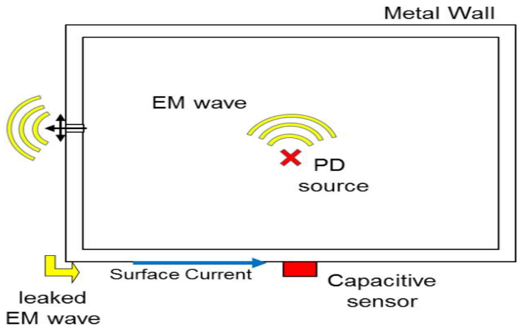
When PD occurs inside switchgear, electromagnetic (EM) waves are emitted. The EM waves propagate and leak to the external surface of the metal tank wall from the dielectric discontinuities (insulator defects, joint, isolated area, bushing, etc.). Then, the surface current generated by EM waves is excited and flows to the ground. Such propagating electromagnetic waves can be obtained by capacitive sensor and recorded as TEV signals [
21,
22,
23]. These sensors pick-up the high frequency (radio frequency) pulses in the frequency range of 4 MHz to 100 MHz.
Figure 1 illustrates the mechanism of generation and detection of transient earth voltage.
3. Experimental Setup and Method
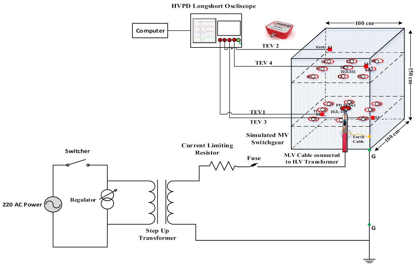
Experiments were conducted by using an experimental setup using the TEV PD detection system shown in
Figure 2. The system consists of,
- (I)
an enclosed steel tank of (100 × 100 × 150 cm) dimensions,
- (II)
a PD source (needle electrode) placed in 18 different locations inside tank (one location at a time),
- (III)
an array of TEV sensors,
- (IV)
a HVPD digital oscilloscope,
- (V)
a 50 kVA step-up transformer and
- (VI)
a current limiting resistor.
Four TEV sensors were mounted on the surface walls outside the simulated switchgear tank to detect and capture the PD signals generated by the PD source inside tank. Their outputs were connected to a 5 GS/s four-channel HVPD® digital oscilloscope having a 400 MHz bandwidth via 5 M long coaxial cables of identical electrical length so that any difference in arrival time between two signals can only be caused by different path lengths inside switchgear tank. The HVPD TEV sensors used has bandwidth of 4~100 MHz.
A needle electrode with tip radius 1 mm (approx.) mounted at the end of a MV power cable was used as the PD source. Eighteen different locations were selected for the needle electrode to generate PD signals. The applied voltage was gradually increased at steps of about 2 kV/sec until the first PD signal was detected by TEV sensor and was recorded on the HVPD digital oscilloscope. The measured partial discharge inception voltage (PDIV) was 21.5 kV, representing the RMS value.
The coordinates of the TEV sensors (S1~S4) and PD sources with respect to the axis as defined in
Figure 3 are given in
Table 1 and
Table 2, respectively. The
X-axis indicates the position parallel to the length of switchgear panel and the
Y-axis indicates the position parallel to the width of switchgear panel, whereas the
Z-axis indicates the height of switchgear panel.
The experiments were performed at the High Voltage laboratory of King Saud University (KSU), which is completely covered with faraday mesh that has very minor/negligible external noise effects.
Each PD test was repeated at least 10 times for each PD source location and were recorded and used in the analysis.
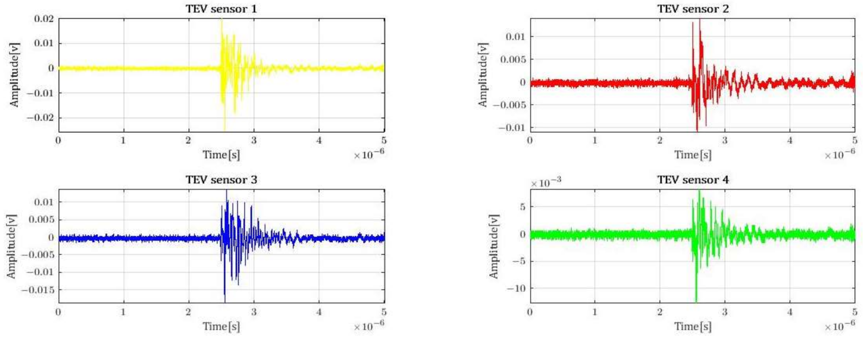
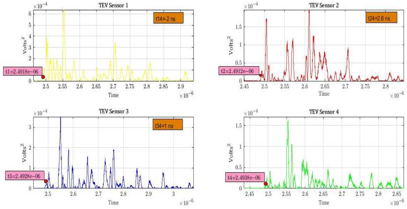
Figure 4 shows an example of captured TEV signals of data sampled. PD waveforms were recorded from four TEV sensors in 18 different locations. Consequently, 720 sets (= 18 × 4 × 10) of PD signals were obtained. The comma-separated values (CSV) in excel files of these waveform sets were imported to MATLAB program 2017 b to determine the TDOA for each PD location.
4. PD Data and its Analysis Technique
Figure 3 shows the 3-D view of the test switchgear panel that indicated 18 PD needle shaped defect sources and four TEV sensors (S1−S4) mounted on the walls outside the switchgear for triangulation. The method of locating signals in each axis starts from the
X-axis and
Z-axis, and is followed by
Y-axis.
TEV signals describe the degree of partial discharge activity by providing information about the signal amplitude against time. Therefore, two approaches can be used for PD localization. One is signal amplitude or received signal strength detection and the second is the measurements of time of arrivals of signals from different locations known as triangulation [
6,
10]. It is based on the TDOA measurement of the PD signals from the known locations of the TEV sensors. It will result in the ability to locate the target node of the PD source. Trilateration is the measurement of the signal time of flight from various locations to locate the source of the PD signal.
The distance between the PD source and the j
th sensor may be represented by the Pythagorean theorem as per Equation (1), where
are the coordinates of the j
th sensor and
are the coordinates of the know PD source location.
According to [
24,
25], the PD source coordinates can be expressed in terms of the distance between the reference sensor and the PD source when the PD signals are captured at multiple sensors.
For a four-TEV sensors system, where the number of measurements is equal to the number of unknowns, considering the TEV sensor 4 as the reference sensor, the location of PD source can be estimated and written as in Equation (2):
In Equation (2), is the coordinates distance of the jth sensor to reference sensor 4 (j = 1, 2, 3). is the TDOA between the jth sensor and reference sensor 4 multiplied by the propagation speed of light (3 × m/s). is the distance of reference sensor 4 to the PD source.
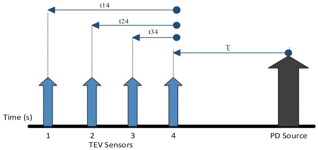
As described in the principles of the TEV method in
Section 2, when the PD occurs inside the switchgear tank, electromagnetic waves are emitted and generated. The electromagnetic waves propagate from the PD source to the external surface of the metal tank wall and arrive at the different TEV sensors at different instants of time. This is demonstrated in
Figure 5 with the support of a four-TEV sensors system. The PD source is located nearer to sensor 4 as compared to Sensor S3, S2 and S1. Consequently, the PD signal arrives at S4 first. The time of arrival (TOA) of the TEV signal, which taken from the PD source to S4, has been denoted as
,
denotes the TOA from the PD source to S3,
denotes the TOA from the PD source to S2 and
denotes the TOA from the PD source to S1. The TDOA between the two sensors S4 and
is
and is given by Equation (4).
The time taken from PD source to nearest TEV sensor is denoted Ʈ as depicted in
Figure 5.
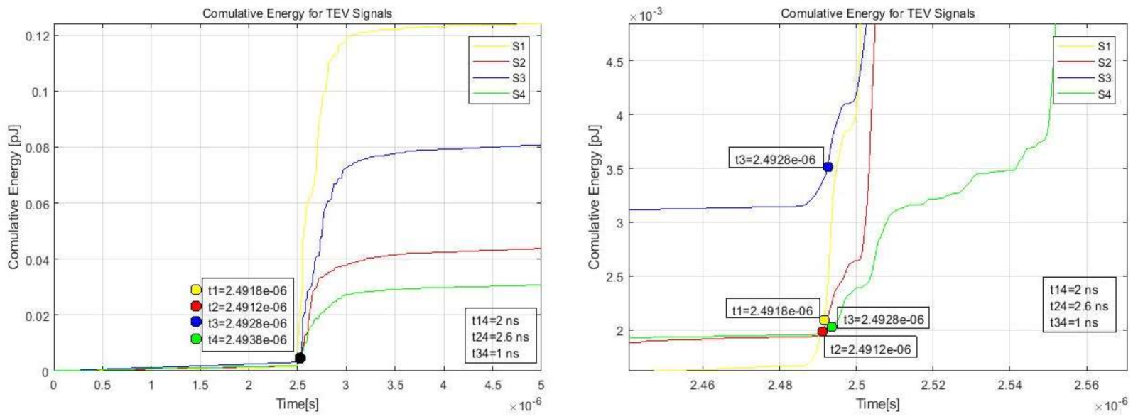
The background noise and initial oscillation in the acquired waveforms makes the analysis more difficult and complicated. In addition, the propagation velocity in the air is so fast that a minor error can result in great errors in the localization of the PD source. Hence, it is difficult to determine the arrival time precisely as well as PD location based on the first peak or knee point method. In order to avoid the errors in the arrival time’s estimation, CEM is used in the analysis; it has two steps.
Non-linear TDOA equations are solved according to Equations (1)–(5) above, to estimate the coordinates of PD source and compare the results with the actual PD source coordinates.
The MATALAB Code is built to find the PD location based on Equations (1)–(4).
Figure 8 illustrates the flow chart diagram that demonstrates the program procedures.
5. Results and Discussions
Table 3 shows the expected TDOA between each TEV sensor pair when the PD source is placed at different locations inside switchgear tank. The expected TOA is calculated for each TEV sensor using Equation (6).
Table 4 illustrates the estimated TDOA by CEM method as discussed in
Section 4, whereas
Table 5 compares the expected TDOA with the estimated TDOA by measuring the TDOA error between them using Equation (7) to determine the PD location accuracy of the TEV detection system.
The lowest average errors of time difference were (0.85 ns) between signals captured by S1−S3 and were (1.12 ns) between signal captured by S2−S4. This is because the signals of sensors 1 and 3 and the signals of sensors 2 and 4 have similar waveform patterns to each other and, thus, produce similar cumulative energy curves. This means the PD signals patterns are very much affected by the sensor locations. The sensors 1 and 3 are located in the bottom level of tank and sensors 2 and 4 are located in the upper level of tank.
As indicated in
Table 5 above, the highest average errors of time difference was about 4.65 ns, followed by 4.018 ns, 3.49 ns and 2.63 ns between signals captured by sensors S3−S4, S1−S4, S2−S3 and S1−S2, respectively. This is because sensors are located at different levels of the tank, which produce the dissimilarity in waveform patterns and leads to increased error.
In addition, sensors S1−S3 produce less error than sensors S2−S4 because S1−S3 sensors are near the MV cable entrance hole on the bottom side of the tank that leads them to get PD signals before the S2−S4 sensors, as well as the initial wave front of the field radiated by the PD source is not uniform in all directions.
Furthermore, the experiments have been applied on a simple empty switchgear tank, which made the task of measuring arrival times more complicated since there are no internal components to diversify the orientation of the electric field. In addition, it may be due to the occurrence of the electromagnetic waves reflections occurrence with the internal tank walls during the propagation that caused distortion to PD signal waveform.
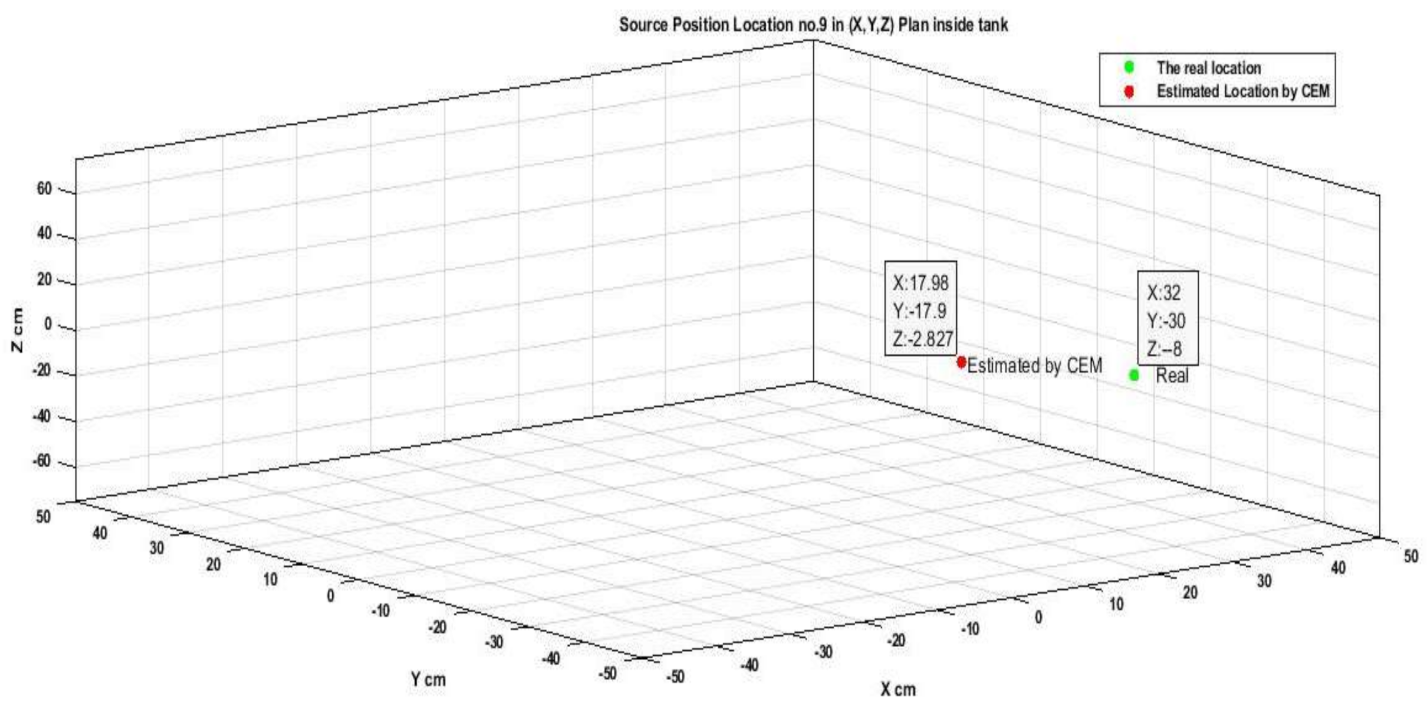
With the assumption that the PD signal travels in the shortest path (a straight line), the closest sensor should receive the signal first and the furthest sensor should pick up the signal last. Thus, for the PD signal generated at location No.9 as an example, sensor 3 should receive the signal first, followed by sensor 1, 2 and finally by sensor 4. Nevertheless, the estimated sequence for PD signal generated at location No.9 indicates that S2 received the signal earlier than S1, followed by S3 and S4. For PD signals in 18 locations, cumulative energy curves give incorrect sequences in all the PD locations except PD location No.1 and PD location No.5.
The average error produced by using the CEM method to estimate the arrival time of a TEV signal was ±1.34 ns, approximately. This is equivalent to a propagation distance of 40.2 cm or (0.40 m), in air, where the velocity of the signal in air is equivalent to the speed of light (0.3 m/ns).
Based on the obtained results mentioned above,
Table 6 illustrates the estimated coordinate of the PD source location in the 3-D space inside the switchgear tank and its comparison with known coordinates of the PD source location (
Table 2) to measure root mean square error (RMSE) using Equation (8).
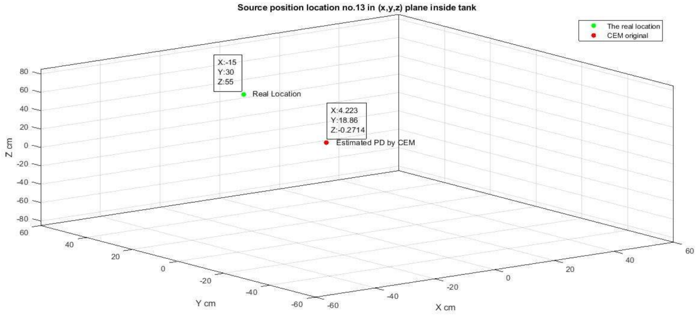
As shown in
Table 6, different PD source locations show coordinates inside the switchgear tank. The minimum RMSE was 19.22 cm for the PD signal generated at location No.9, and the highest RMSE was 59.5 cm for the PD signal generated at location No.13. The overall average error produced by using the CEM method to estimate the arrival time of a TEV signal for 18 locations was 40.2 cm (0.40 m) and corresponds to 1.34 ns in the signal propagation time.
Figure 9 and
Figure 10 illustrate the PD localization error that shows the coordinates of the actual PD source as well as the location estimates obtained from CEM in the 3-D space inside the switchgear tank for the PD signal generated at location No.9 and for PD location No.13, respectively.
6. Conclusions
This paper discussed the accuracy of the PD source localization method inside a switchgear tank by using an array of TEV sensors. The Cumulative Energy Method was used for estimating the time difference of arrival of the PD signal generated by a needle shaped electrode mounted at 18 different locations inside a simulated tank. These signals were captured by four TEV sensors mounted at four different locations on the walls of the tank. The onset time using the CEM method was determined corresponding to five percent (0.05) of the maximum value of or cumulative energy. This method was effective for estimating the onset time of the TEV signals producing values that differs from the expected ones by 1.34 ns on average. The average RMSE error was 40.2 cm and corresponds to the average error of TDOA, 1.34 ns.
The results show that TDOA are affected by sensor positions where the error in TDOA increased when sensors were installed in different levels of the tank and reduced when sensors were installed in the same level.
In addition, the results have shown an incorrect sequence of receiving signals in all PD locations except locations No.1 and 5. This means distortion occurred to signal waveforms because of the electromagnetic waves reflections during its propagation since the tank is empty and there are no internal components to diversify the orientation of the electric field.
In the future research, a study will be carried out to measure the accuracy of PD localization inside a switchgear tank by the receiving signal strength (RSS) method and compare it with the TDOA method.


