Multivariable Deadbeat Control of Power Electronics Converters with Fast Dynamic Response and Fixed Switching Frequency

 ,
,  ,
,  ,
, 

Abstract
1. Introduction
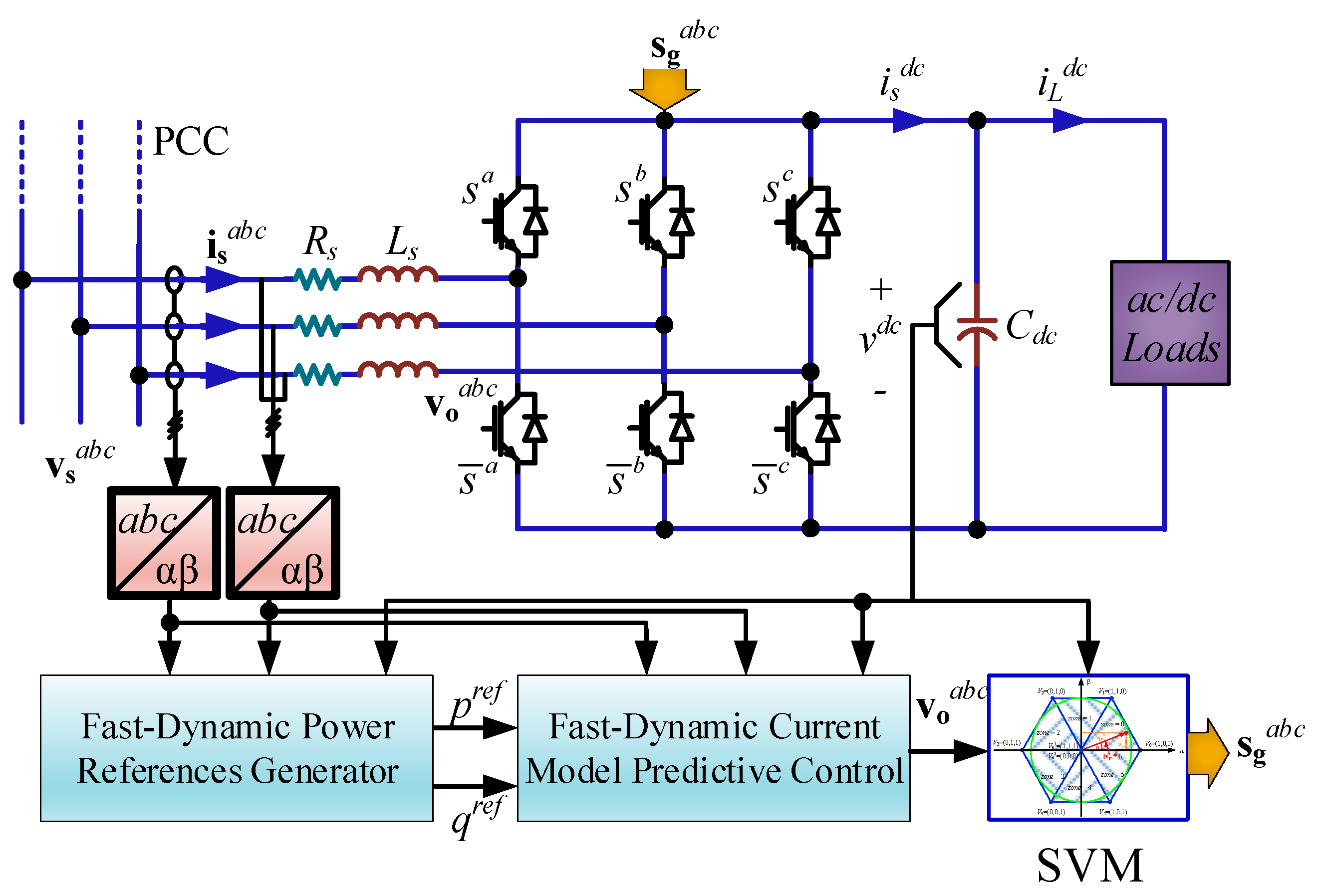
2. System Modelling
2.1. Continuous Static Reference Frame Model
2.2. Discrete Static Reference Frame Model
3. Predictive Control Strategy
3.1. Power Converter Voltage
3.2. Current References as a Function of the Power Reference
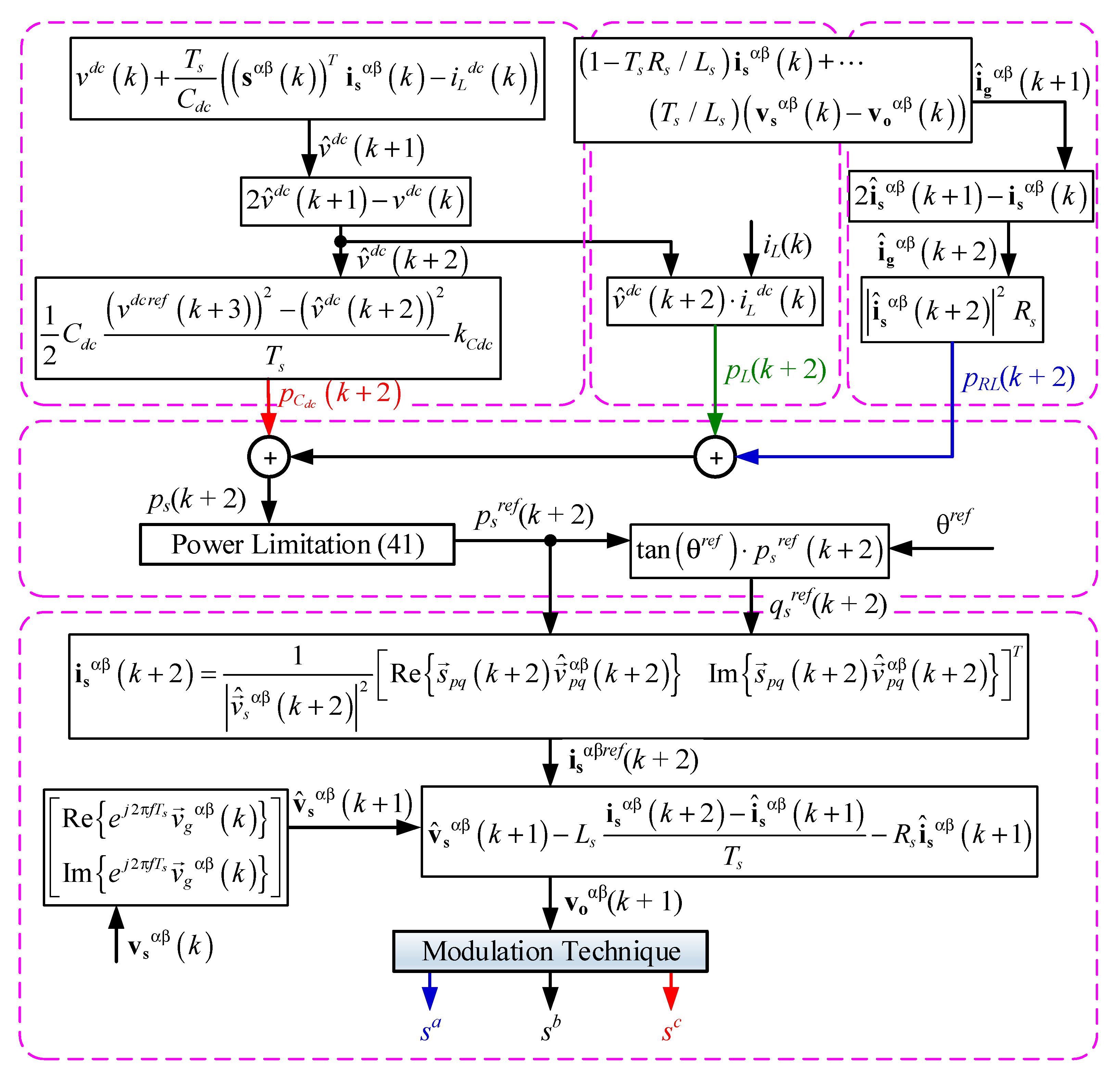
3.3. Power Reference Calculation
- -
- dc load power consumption: This contribution represents what the power converter is supplying to the dc loads through the current iLdc. The related dc power is computed as:
- -
- ac inductive filter losses: The filter included on the ac side has natural losses, associated to Rs, due to the non-ideality of the inductance, and can be calculated as:
- -
- Power supplied to the dc capacitor: The dc link capacitor Cdc is charged/discharged in order to maintain the dc voltage to its reference. Therefore, this power is regulated by the dc voltage control. The energy on the dc capacitor at time t is given by:
4. Multivariable Fast-Dynamic Deadbeat Control
5. Simulation and Experimental Results
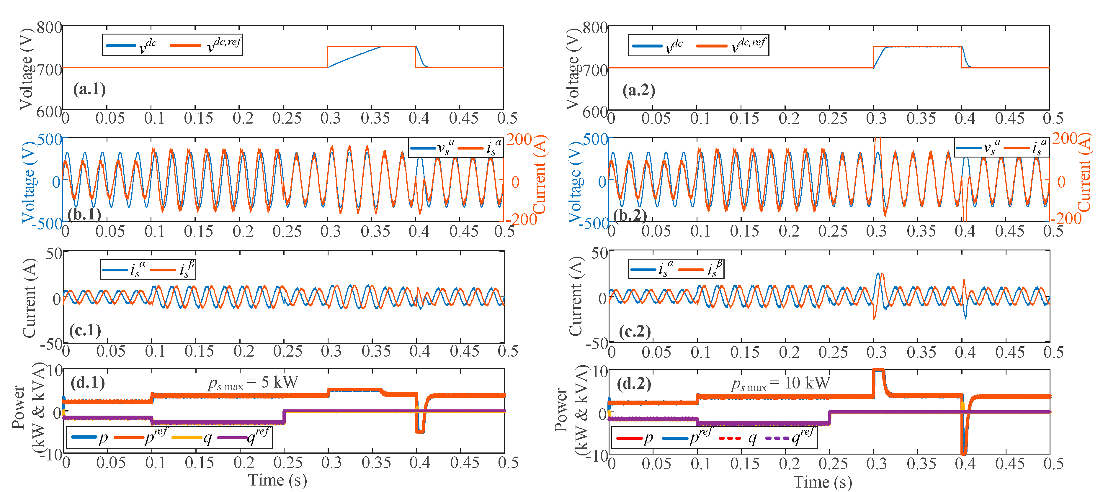
5.1. Simulative Results
5.2. Response under Model Uncertainties
5.3. Experimental Tests
6. Conclusions
Author Contributions
Funding
Conflicts of Interest
References
- Moradi, M. Predictive control with constraints, J.M. Maciejowski; Pearson Education Limited, Prentice Hall, London, 2002, pp. IX+331, price £35.99, ISBN 0-201-39823-0. Int. J. Adapt. Control. Signal Process. 2003, 17, 261–262. [Google Scholar] [CrossRef]
- Rosa, F.C.; Bim, E. A Constrained Non-Linear Model Predictive Controller for the Rotor Flux-Oriented Control of an Induction Motor Drive. Energies 2020, 13, 3899. [Google Scholar] [CrossRef]
- Bemporad, A.; Borrelli, F.; Morari, M. Model predictive control based on linear programming—The explicit solution. IEEE Trans. Autom. Control. 2002, 47, 1974–1985. [Google Scholar] [CrossRef]
- Tinazzi, F.; Carlet, P.G.; Bolognani, S.; Zigliotto, M. Motor Parameter-Free Predictive Current Control of Synchronous Motors by Recursive Least-Square Self-Commissioning Model. IEEE Trans. Ind. Electron. 2019, 67, 9093–9100. [Google Scholar] [CrossRef]
- Tavernini, D.; Metzler, M.; Gruber, P.; Sorniotti, A. Explicit Nonlinear Model Predictive Control for Electric Vehicle Traction Control. IEEE Trans. Control. Syst. Technol. 2019, 27, 1438–1451. [Google Scholar] [CrossRef]
- Ma, M.; Liu, X.; Lee, K.Y. Maximum Power Point Tracking and Voltage Regulation of Two-Stage Grid-Tied PV System Based on Model Predictive Control. Energies 2020, 13, 1304. [Google Scholar] [CrossRef]
- Martinek, R.; Rzidky, J.; Jaros, R.; Bilik, P.; Ladrova, M. Least Mean Squares and Recursive Least Squares Algorithms for Total Harmonic Distortion Reduction Using Shunt Active Power Filter Control. Energies 2019, 12, 1545. [Google Scholar] [CrossRef]
- Rodriguez, J.R.; Kazmierkowski, M.P.; Espinoza, J.R.; Zanchetta, P.; Abu-Rub, H.; Young, H.A.; Rojas, C.A. State of the Art of Finite Control Set Model Predictive Control in Power Electronics. IEEE Trans. Ind. Inform. 2013, 9, 1003–1016. [Google Scholar] [CrossRef]
- Gonçalves, P.F.; Cruz, S.M.; Mendes, A.M.S. Finite Control Set Model Predictive Control of Six-Phase Asymmetrical Machines—An Overview. Energies 2019, 12, 4693. [Google Scholar] [CrossRef]
- Singh, V.; Tripathi, R.; Tsuyoshi, H. FPGA-Based Implementation of Finite Set-MPC for a VSI System Using XSG-Based Modeling. Energies 2020, 13, 260. [Google Scholar] [CrossRef]
- Bigarelli, L.; Di Benedetto, M.; Lidozzi, A.; Solero, L.; Odhano, S.A.; Zanchetta, P. PWM-Based Optimal Model Predictive Control for Variable Speed Generating Units. IEEE Trans. Ind. Appl. 2019, 56, 541–550. [Google Scholar] [CrossRef]
- Guzmán, R.; De Vicuna, L.G.; Castilla, M.; Miret, J.; Camacho, A. Finite Control Set Model Predictive Control for a Three-Phase Shunt Active Power Filter with a Kalman Filter-Based Estimation. Energies 2017, 10, 1553. [Google Scholar] [CrossRef]
- Liu, X.; Wang, D.; Peng, Z. Cascade-Free Fuzzy Finite-Control-Set Model Predictive Control for Nested Neutral Point-Clamped Converters with Low Switching Frequency. IEEE Trans. Control. Syst. Technol. 2018, 27, 2237–2244. [Google Scholar] [CrossRef]
- Toledo, S.; Maqueda, E.; Rivera, M.; Gregor, R.; Wheeler, P.; Romero, C. Improved Predictive Control in Multi-Modular Matrix Converter for Six-Phase Generation Systems. Energies 2020, 13, 2660. [Google Scholar] [CrossRef]
- Bao, G.; Qi, W.; He, T. Direct Torque Control of PMSM with Modified Finite Set Model Predictive Control. Energies 2020, 13, 234. [Google Scholar] [CrossRef]
- Tarisciotti, L.; Lei, J.; Formentini, A.; Trentin, A.; Zanchetta, P.; Wheeler, P.; Rivera, M. Modulated Predictive Control for Indirect Matrix Converter. IEEE Trans. Ind. Appl. 2017, 53, 4644–4654. [Google Scholar] [CrossRef]
- Tarisciotti, L.; Formentini, A.; Gaeta, A.; Degano, M.; Zanchetta, P.; Rabbeni, R.; Pucci, M. Model Predictive Control for Shunt Active Filters with Fixed Switching Frequency. IEEE Trans. Ind. Appl. 2017, 53, 296–304. [Google Scholar] [CrossRef]
- Yeoh, S.S.; Yang, T.; Tarisciotti, L.; Hill, C.I.; Bozhko, S.; Zanchetta, P. Permanent-Magnet Machine-Based Starter–Generator System with Modulated Model Predictive Control. IEEE Trans. Transp. Electrif. 2017, 3, 878–890. [Google Scholar] [CrossRef]
- Garcia, C.; Silva, C.A.; Rodriguez, J.; Zanchetta, P.; Odhano, S.A. Modulated Model-Predictive Control with Optimized Overmodulation. IEEE J. Emerg. Sel. Top. Power Electron. 2019, 7, 404–413. [Google Scholar] [CrossRef]
- Agustin, C.A.; Yu, J.-T.; Lin, C.-K.; Fu, X.-Y. A Modulated Model Predictive Current Controller for Interior Permanent-Magnet Synchronous Motors. Energies 2019, 12, 2885. [Google Scholar] [CrossRef]
- Nguyen, T.H.; Kim, K.-H. Finite Control Set–Model Predictive Control with Modulation to Mitigate Harmonic Component in Output Current for a Grid-Connected Inverter under Distorted Grid Conditions. Energies 2017, 10, 907. [Google Scholar] [CrossRef]
- Kawabata, T.; Miyashita, T.; Yamamoto, Y. Dead Beat Control of Three Phase PWM Inverter. In Proceedings of the 1987 IEEE Power Electronics Specialists Conference, Blacksburg, VA, USA, 21–26 June 1987; pp. 473–481. [Google Scholar]
- Danayiyen, Y.; Lee, K.; Choi, M.; Lee, Y.I. Model Predictive Control of Uninterruptible Power Supply with Robust Disturbance Observer. Energies 2019, 12, 2871. [Google Scholar] [CrossRef]
- Zhang, Y.; Du, G.; Li, J.; Lei, Y. Hybrid Control Strategy of MPC and DBC to Achieve a Fixed Frequency and Superior Robustness. Energies 2020, 13, 1176. [Google Scholar] [CrossRef]
- Malesani, L.; Mattavelli, P.; Buso, S. Robust dead-beat current control for PWM rectifiers and active filters. IEEE Trans. Ind. Appl. 1999, 35, 613–620. [Google Scholar] [CrossRef]
- Kim, J.; Hong, J.; Kim, H.-J. Improved Direct Deadbeat Voltage Control with an Actively Damped Inductor-Capacitor Plant Model in an Islanded AC Microgrid. Energies 2016, 9, 978. [Google Scholar] [CrossRef]
- Abdelrahem, M.; Hackl, C.M.; Rodriguez, J.; Kennel, R. Model Reference Adaptive System with Finite-Set for Encoderless Control of PMSGs in Micro-Grid Systems. Energies 2020, 13, 4844. [Google Scholar] [CrossRef]
- Tang, M.; Gaeta, A.; Ohyama, K.; Zanchehtta, P.; Asher, G. Assessments of Dead Beat Current Control for High Speed Permanent Magnet Synchronous Motor Drives. In Proceedings of the 9th International Conference on Power Electronics and ECCE Asia (ICPE-ECCE Asia), Seoul, Korea, 1–5 June 2015; pp. 1867–1874. [Google Scholar]
- Huang, Q.; Shen, G.; Min, R.; Tong, Q.; Zhang, Q.; Liu, Z. State Switched Discrete-Time Model and Digital Predictive Voltage Programmed Control for Buck Converters. Energies 2020, 13, 3451. [Google Scholar] [CrossRef]
- Scarcella, G.; Scelba, G.; Pulvirenti, M.; Lorenz, R.D. Fault-Tolerant Capability of Deadbeat-Direct Torque and Flux Control for Three-Phase PMSM Drives. IEEE Trans. Ind. Appl. 2017, 53, 5496–5508. [Google Scholar] [CrossRef]
- Xing, X.; Zhang, C.; Chen, A.; Geng, H.; Qin, C. Deadbeat Control Strategy for Circulating Current Suppression in Multiparalleled Three-Level Inverters. IEEE Trans. Ind. Electron. 2018, 65, 6239–6249. [Google Scholar] [CrossRef]
- Heydari, E.; Varjani, A.Y.; Diallo, D. Fast terminal sliding mode control-based direct power control for single-stage single-phase PV system. Control. Eng. Pract. 2020, 104, 104635. [Google Scholar] [CrossRef]
- Wang, P.; Bi, Y.; Gao, F.; Song, T.; Zhang, Y. An Improved Deadbeat Control Method for Single-Phase PWM Rectifiers in Charging System for EVs. IEEE Trans. Veh. Technol. 2019, 68, 9672–9681. [Google Scholar] [CrossRef]
- Rovere, L.; Formentini, A.; Zanchetta, P. FPGA Implementation of a Novel Oversampling Deadbeat Controller for PMSM Drives. IEEE Trans. Ind. Electron. 2018, 66, 3731–3741. [Google Scholar] [CrossRef]
- Kang, S.-W.; Soh, J.-H.; Kim, R.-Y. Symmetrical Three-Vector-Based Model Predictive Control with Deadbeat Solution for IPMSM in Rotating Reference Frame. IEEE Trans. Ind. Electron. 2020, 67, 159–168. [Google Scholar] [CrossRef]
- Wang, Y.; Li, K.; Liu, X. Improved Deadbeat Control for PMSM with Terminal Sliding Mode Observer. In Proceedings of the 22nd International Conference on Electrical Machines and Systems (ICEMS), Harbin, China, 11–14 August 2019; pp. 1–5. [Google Scholar]
- You, Z.-C.; Huang, C.-H.; Yang, S.-M. Online Current Loop Tuning for Permanent Magnet Synchronous Servo Motor Drives with Deadbeat Current Control. Energies 2019, 12, 3555. [Google Scholar] [CrossRef]
- Abdelrahem, M.; Rodriguez, J.; Kennel, R. Improved Direct Model Predictive Control for Grid-Connected Power Converters. Energies 2020, 13, 2597. [Google Scholar] [CrossRef]
- Mattavelli, P. An Improved Deadbeat Control for UPS Using Disturbance Observers. IEEE Trans. Ind. Electron. 2005, 52, 206–212. [Google Scholar] [CrossRef]
- Springob, L.; Holtz, J. High-bandwidth current control for torque-ripple compensation in PM synchronous machines. IEEE Trans. Ind. Electron. 1998, 45, 713–721. [Google Scholar] [CrossRef]
- Oleschuk, V.; Ermuratskii, V. Multi-Inverter Drive with Symmetrical Multilevel Winding Voltage of Transformer during Overmodulation. In Proceedings of the 5th International Symposium on Electrical and Electronics Engineering (ISEEE), Galati, Romania, 20–22 October 2017; pp. 1–4. [Google Scholar]
- Munoz, J.A.; Reyes, J.R.; Espinoza, J.R.; Rubilar, I.A.; Moran, L.A. A Novel Multi-Level Three-Phase UPQC Topology Based on Full-Bridge Single-Phase Cells. In Proceedings of the IECON 2007—33rd Annual Conference of the IEEE Industrial Electronics Society, Taipei, Taiwan, 5–8 November 2007; pp. 1787–1792. [Google Scholar]
- Rettner, C.; Schiedermeier, M.; Apelsmeier, A.; Marz, M. Fast DC-Link Capacitor Design for Voltage Source Inverters Based on Weighted Total Harmonic Distortion. In Proceedings of the 2020 IEEE Applied Power Electronics Conference and Exposition (APEC), New Orleans, LA, USA, 15–19 March 2020; pp. 3520–3526. [Google Scholar]
- Chien, W.-S.; Tzou, Y.-Y. Analysis and Design on the Reduction of DC-Link Electrolytic Capacitor for AC/DC/AC Converter Applied to AC Motor Drives. In Proceedings of the PESC 98—29th Annual IEEE Power Electronics Specialists Conference, Fukuoka, Japan, 22 May 1998; Volume 1, pp. 275–279. [Google Scholar]
- Townsend, C.D.; Yu, Y.; Konstantinou, G.; Agelidis, V.G. Cascaded H-Bridge Multilevel PV Topology for Alleviation of Per-Phase Power Imbalances and Reduction of Second Harmonic Voltage Ripple. IEEE Trans. Power Electron. 2015, 31, 5574–5586. [Google Scholar] [CrossRef]
- Galassini, A.; Calzo, G.L.; Formentini, A.; Gerada, C.; Zanchetta, P.; Costabeber, A. uCube: Control Platform for Power Electronics. In Proceedings of the 2017 IEEE Workshop on Electrical Machines Design, Control and Diagnosis (WEMDCD), Nottingham, UK, 20–21 April 2017; pp. 216–221. [Google Scholar]


| Parameters | Value |
|---|---|
| vs (grid nominal voltage value) | 230 V, rms |
| vdc (dc link nominal voltage) | 700 V |
| Rs (filter resistance) | 0.4 Ω |
| Ls (filter inductance) | 4.75 mH |
| Cdc (dc link capacitor) | 2.2 mF |
| fs (grid frequency) | 50 Hz |
| Ts (controller sampling time) | 50 µs |
| fsw (switching frequency) | 20 kHz |
| Tm (controller parameter) | 25 p.u. |
Publisher’s Note: MDPI stays neutral with regard to jurisdictional claims in published maps and institutional affiliations. |
© 2021 by the authors. Licensee MDPI, Basel, Switzerland. This article is an open access article distributed under the terms and conditions of the Creative Commons Attribution (CC BY) license (http://creativecommons.org/licenses/by/4.0/).
Share and Cite
Rohten, J.A.; Dewar, D.N.; Zanchetta, P.; Formentini, A.; Muñoz, J.A.; Baier, C.R.; Silva, J.J. Multivariable Deadbeat Control of Power Electronics Converters with Fast Dynamic Response and Fixed Switching Frequency. Energies 2021, 14, 313. https://doi.org/10.3390/en14020313
Rohten JA, Dewar DN, Zanchetta P, Formentini A, Muñoz JA, Baier CR, Silva JJ. Multivariable Deadbeat Control of Power Electronics Converters with Fast Dynamic Response and Fixed Switching Frequency. Energies. 2021; 14(2):313. https://doi.org/10.3390/en14020313
Chicago/Turabian StyleRohten, Jaime A., David N. Dewar, Pericle Zanchetta, Andrea Formentini, Javier A. Muñoz, Carlos R. Baier, and José J. Silva. 2021. "Multivariable Deadbeat Control of Power Electronics Converters with Fast Dynamic Response and Fixed Switching Frequency" Energies 14, no. 2: 313. https://doi.org/10.3390/en14020313
APA StyleRohten, J. A., Dewar, D. N., Zanchetta, P., Formentini, A., Muñoz, J. A., Baier, C. R., & Silva, J. J. (2021). Multivariable Deadbeat Control of Power Electronics Converters with Fast Dynamic Response and Fixed Switching Frequency. Energies, 14(2), 313. https://doi.org/10.3390/en14020313