Analysis of the Electricity Supply Contracts for Medium-Voltage Apartments in the Republic of Korea

Abstract

For apartment complexes receiving medium-voltage electrical energies, the apartments can choose an electricity charging method between the single and general contracts in the Republic of Korea. In the single contract, a residential high-voltage rate is applied to the total electrical energy consumptions of households and common areas. On the other hand, in the general contract, different rate plans are applied to the electrical energy consumptions of households and their common areas, where a generic high-voltage rate plan is applied to the common consumption. Hence, depending on the amounts and composition of the consumptions, both contracts have their own strengths and weaknesses in terms of the total electricity charge. The management office of an apartment complex can select its preferred contract considering the amount and composition of the power consumptions on an annual basis. In this paper, we first formulate a model for the contracts and analyze their properties based on Monte-Carlo simulations. We then observe the contract properties through actual metering data from 30 apartment complexes in Korea. From the analysis of this paper, we can select appropriate contract for a given apartment complex and have guidelines for saving electricity charges. The greater the consumption of the electrical energy and the common area portion, the more advantageous the general contract is in terms of reducing electricity charges.

1. Introduction

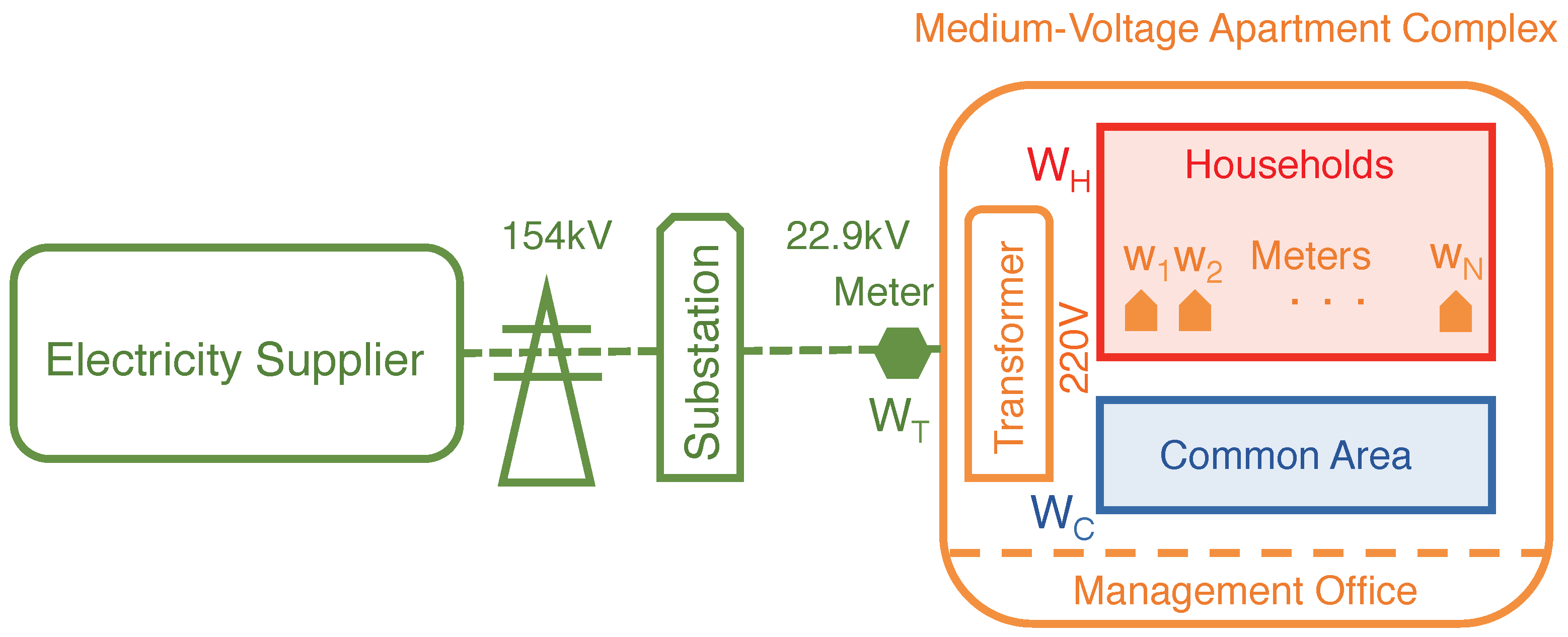
In the Republic of Korea, different electricity rates are operated depending on their purposes, such as residential, educational, industrial, agricultural, street lamp, and generic uses. These six rates have their own rate systems [1]. Depending on the provided voltage levels, the electricity rates can also be classified into the high-voltage or low-voltage rate. For the residential rate, we have the residential high-voltage and low-voltage rates. For the cases of detached houses and multifamily houses, the electricity suppliers, such as the Korea Electric Power Corporation (KEPCO), lower a medium voltage of 22.9 kV into a low-voltage of 220 V to provide electrical energy. On the other hand, apartment complexes directly receive electrical energy, which has a medium voltage of 22.9 kV. The apartment complexes then lower the incoming medium voltage into a low voltage of 220 V by using their electrical power facilities, which are maintained by the apartment management offices. Here, maintaining electricity energy meters and reading the meters are operated by the management office as shown in Figure 1 [2,3,4]. Here, the advanced metering infrastructure (AMI) can efficiently provide metering data to the apartment management offices as well as electricity suppliers.

The detached houses, which receive low-voltage electrical energies from electricity suppliers, have the electricity charges, which are calculated from the corresponding electricity energy meters [5,6]. Here, the electricity meters are installed and maintained by the electricity suppliers. On the other hand, medium-voltage apartment complexes have common electricity usages from common areas, such as parking lots, elevators, and security offices besides the household electricity usage as shown in Figure 1. Depending on how to manage this common electricity usage, there are two contracts, which are called the single and general contracts, for the medium-voltage apartment complexes. In the single contract, an average electricity usage is first calculated from summing the usages of households and common areas and then dividing it by the number of households. The electricity charge is calculated from applying the residential high-voltage electricity rate to the average then multiplying it by the number of households. Because only one electricity rate is applied to the total usage in a simple manner, the single contract has advantages of simple and unified calculations. Furthermore, reading from a meter, which is attached to the entering power line to the apartment complex, is enough to calculate the electricity charge [7,8,9]. However, the single contract has the disadvantage of charge calculations, which are dependent on the usage of other households. In the general contract, compared to the unified calculation of the single contract, electricity charges from the households and common areas are separately calculated to implement a fair independent charge system. For the household electricity usage, the residential low-voltage electricity rate is applied, and for the common electricity usage, the generic high-voltage electricity rate is applied. Depending on the amounts of the household and common usages, the single and general contracts can yield different total electricity charges. Hence, an apartment complex can choose an appropriate contract for reducing the electricity charge. In Korea, the contract can be changed between the single and general contracts on a yearly basis by majority vote of the residents.

The residential electricity rates have progressive properties to restrain electricity usages based on an average electricity energy. In order to solve problems from the progressive residential electricity rate, Kim [10] proposed reasonable residential electricity pricing systems that consider the time-of-unit and real-time pricing concepts to reflect variations in the wholesale electricity price. Yoo et al., [11] studied that the residential electricity demands depend on various factors, such as the size of family, size of house, and household income. For the case of Seoul, Korea, Kim [12] also investigated effects of the factors on the electricity usage. The progressive rates of the electricity company and the electricity usages depending on the various factors of the apartment complexes can provide different electricity charges for the current two contracts. In this paper, we introduce the current contracts, the single and general contracts, which show different properties depending on employed progressive rates and various factors. We then formulate a mathematical model for the household electricity usage and analyze the current contracts based on Monte-Carlo (MC) simulations underlying the household electricity usage model. Properties of the single and general contracts are observed by changing the portion of the common usage. The electricity charge from the single contract shows steps as the common usage portion increases due to the large basic rates. These steps can produce steep charge increases even though the increase in usage is very small. For the general contract, if the standard deviation of the household usages increases, then the electricity charge can be increased even though the total electricity usage does not change. Using actual metering data acquired from 30 apartment complexes, the properties of the contracts are also experimentally observed. From these practical experiments, we can observe that the single contract usually yields lower electricity charges compared to the general contract case, which implies an unbalancing property between the two contracts. From the comparison analysis in this paper, we can expect the following concomitant consequences:

• Model-based MC simulations without using detail personal information
• Selection guide between the single and general contracts for an apartment complex
• Checking steep charge increases at the steps on the single contract electricity charge.

The fact that we can analyze the characteristics of an apartment complex without using person information means that it is practically applicable. By checking the steep charge increases, we can reduce the total electricity charge.

This paper is organized in the following way. In Section 2, we introduce the electricity rates that are employed in the medium-voltage apartment complex. The two contracts, which are provided for the medium-voltage apartment complex, are then introduced with their formulations in Section 3. Analyses based on the MC simulations are introduced in Section 4. In Section 5, actual metering date from 30 apartment complexes are used to analyze the properties of the contracts. The conclusion is then stated in the last section.

2. Rates for the Electricity Usage

In this section, we introduce the residential and generic electricity rates, which are currently used for the electricity contracts for the medium-voltage apartment complexes in Korea [13].

Electricity suppliers use the residential high-voltage and low-voltage rates, and the generic high-voltage rate for the electricity contracts of medium-voltage apartment complexes. The residential high-voltage and low-voltage rates, which are provided by electricity suppliers, such as KEPCO, are summarized in

Table 1. Residential low-voltage electricity rates per month for the summer season (July–August) and the other seasons (January–June and September–December).

Usage Range (kWh)
Other Seasons	Summer	Basic Rate (Won/House)	Usage Rate (Won/kWh)
–200	–300	910	93.3
201–400	301–450	1600	187.9
401–	451–	7300	280.6

and

Table 2. Residential high-voltage electricity rates per month for the summer season (July–August) and the other seasons (January–June and September–December).

Usage Range (kWh)
Other Seasons	Summer	Basic Rate (Won/House)	Usage Rate (Won/kWh)
–200	–300	730	78.3
201–400	301–450	1260	147.3
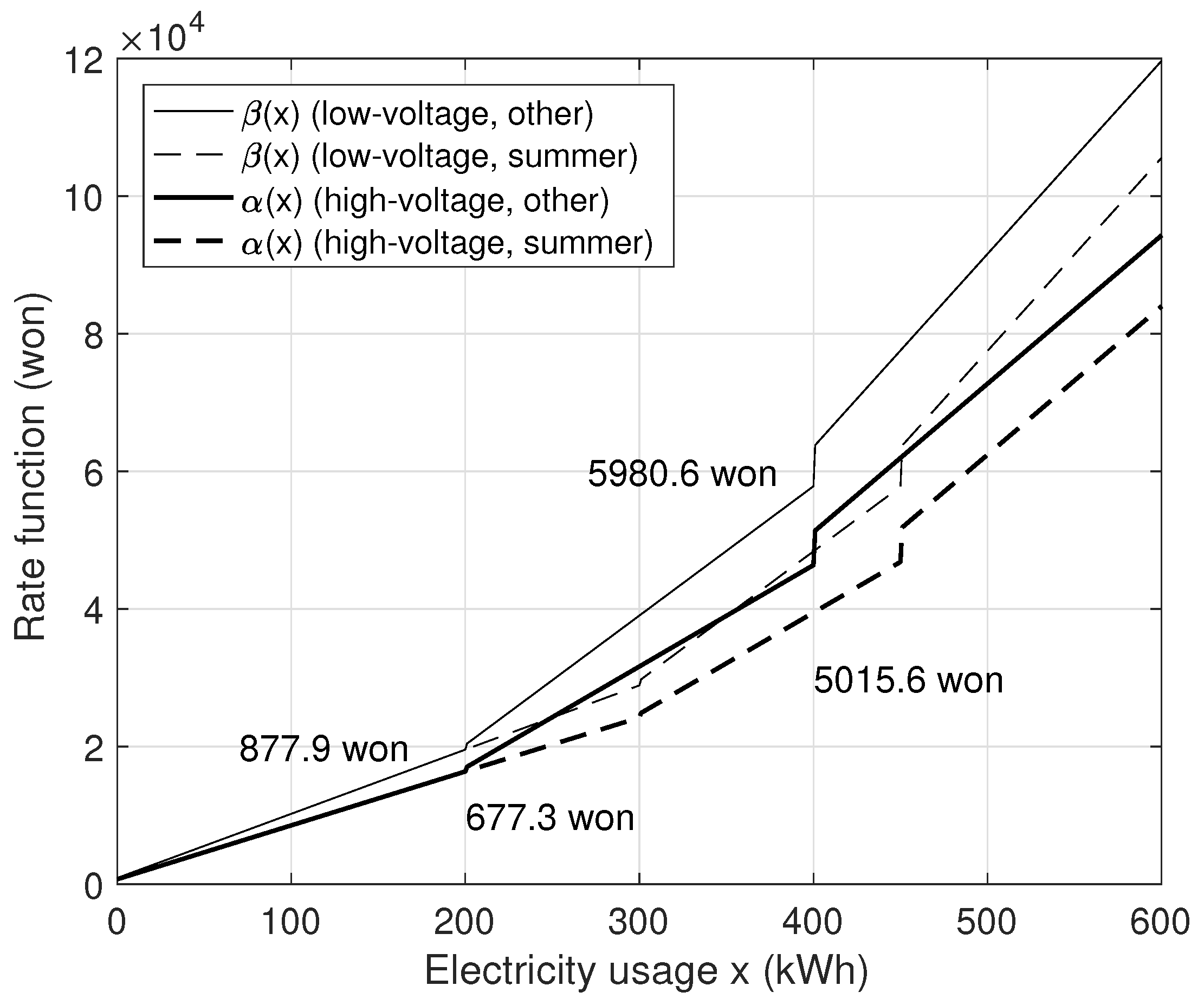
401–	451–	6060	215.6

, respectively. The electricity charges with respect to the electricity usages are illustrated in Figure 2 based on the rates of Table 1 and Table 2. As addressed in the previous section, we can observe from Figure 2 that the electricity charge from the residential high-voltage rate is cheaper than the low-voltage case. The electricity rates are designed based on progressive rate plans and the usage ranges for the summer season are wider than those of other seasons to provide lower electricity rates. This lower rate is politically designed by the government in order to reduce the electricity charges for the summer season. Otherwise, the amount of the electrical energy for cooling can be abnormally increased and thus can yield high electricity charges. For the case of the residential low-voltage rate, if the electricity usage is 450 kWh for the summer season, then 19,795 won per month can be maximally saved compared to the case of other seasons. If the electricity usage is higher than 450 kWh, then a constant 14,095 won will be saved. For the residential high-voltage rate, the maximal saving is reduced to 15,115 won and over the electricity usage of 450 kWh, the constant saving is 10,315 won.

From the electricity rate functions of Figure 2, we can observe that the charge slope or rate increases as the electricity usage range moves to the higher usages based on progressive rate plans. Furthermore, at the discontinuous points between the usage ranges, because of the different basic rates as shown in Table 1 and Table 2, we can observe high electricity charge differences or steps. For example, from the residential low-voltage rate of Table 1, the electricity usages of 200 kWh and 201 kWh, which corresponds to the 1st step, shows an 877.9 won step, which is from the basic rate difference of 690 won (1600-910 ) and the charge of 187.9 won from an 1 kWh usage. For the electricity usages of 400 kWh and 401 kWh, which corresponds to the 2nd step, an 1 kWh usage can increase the charge by 5980.6 won, which is equivalent to a usage of 64.1 kWh for the 1st usage range. For the residential high-voltage rate of Table 2, we can observe similar differences. These abnormal differences at the 2nd step can produce considerable electricity charges. Further observations on the influences from these differences will be introduced in the following sections for the single contract.

In

Table 3. Seasonal generic high-voltage electricity rate per month.

	Usage Rate (Won/kWh)
Basic Rate	Spring and Autumn	Summer	Winter
(Won/kWh)	(March–May, September–October)	(June–August)	(November–February)
8230	67.6	111.9	98.3

, the generic high-voltage electricity rate is summarized. Compared to the residential rates, this general rate does not follow the progressive rate plan. The electricity rate for the spring and autumn seasons has the lowest value of 67.6 won.

3. Single and General Contracts for Medium-Voltage Apartment Complexes

For the medium-voltage apartment complexes, there are two contracts, the single and general contracts, in which three electricity rates of the residential high-voltage, residential low-voltage, and generic high-voltage rates of the previous section are employed. In this section, we formulate these contracts with a household usage model and conduct their analyses based on MC simulations.

We first introduce the electricity usage. Letting $W_T$ denote the total electricity usage in kWh, the total electricity usage can be represented as

$$\begin{array}{c}\hfill W_T:=W_C+W_H.\end{array}$$

(1)

In (1), $W_C$ implies the electricity usage of the common area and $W_H$ implies the total household electricity usage, which can be represented as $W_H=w_1+\cdots +w_N$ as shown in Figure 1. Here, $w_n$ implies the electricity usage of each household in kWh and N denotes the total number of households. Letting $\eta$ denote the common electricity usage portion, we define the portion as

$$\begin{array}{c}\hfill \eta :=\frac{W_C}{W_T},\end{array}$$

(2)

where $0\le \eta <1$ holds. In this paper, we analyze the properties of the single and general contracts by changing the portion $\eta$ for a fixed total household electricity usage of $W_H$.

3.1. Single Contract

In the single contract, we first calculate an average total electricity usage by dividing the total electricity usage by the number of households. We then apply the residential high-voltage rate of Table 2 to the average total electricity usage and calculate the total electricity charge by multiplying the number of households. This charge calculation approach in the single contract is simple because one rate plan, the residential high-voltage rate, is applied to both household and common electricity usages.

We now formulate the total electricity charge in the single contract for a given month. Let $S_T$ denote the total electricity charge per month in the single contract. $S_T$ can then be written as

$$\begin{array}{c}\hfill S_T\left(\eta \right):=N·\alpha \left(W_{AV}\left(\eta \right)\right),\end{array}$$

(3)

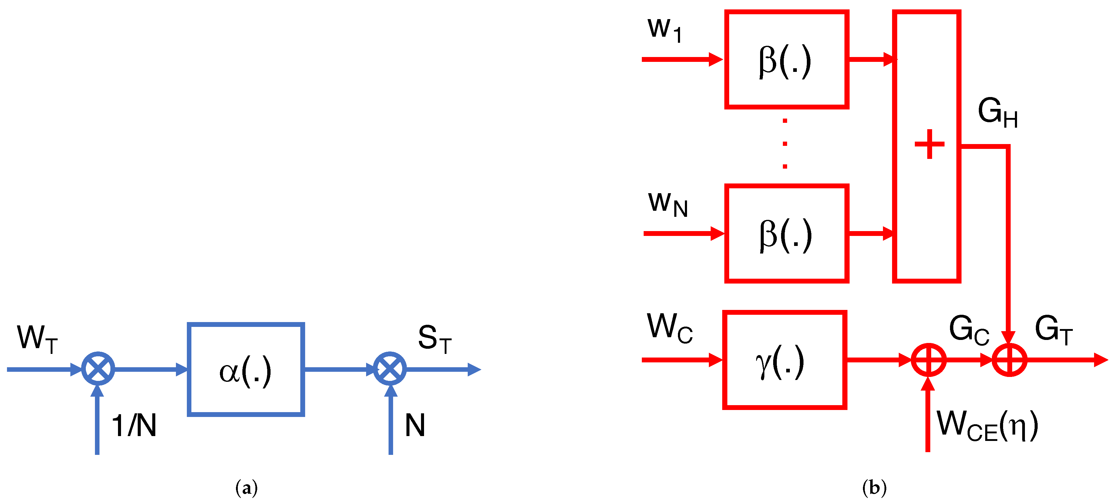
where $W_{AV}$ denotes the average total electricity usage and $\alpha$ is the rate function of the residential high-voltage rate. Here, $W_{AV}$ is calculated from $W_{AV}:=W_T/N$, in which the total electricity usage $W_T$ is measured by an electricity supplier as shown in Figure 1. This calculation is summarized as a block diagram in Figure 3a. For given total household usage $W_H$ and portion $\eta$, the average electricity usage $W_{AV}$ can be rewritten as

$$\begin{array}{c}\hfill W_{AV}\left(\eta \right)=\frac{W_H}{N}\frac{1}{1-\eta }.\end{array}$$

(4)

In (3), the rate function for the other seasons in the residential high-voltage rate can be written as

$$\begin{array}{c}\alpha \left(x\right):=\left\{\begin{array}{cc}730+78.3x\hfill & :\hspace{1em}\le 0\le x\le 200\hfill \\ 1260+78.3\times 200+147.3(x-200)\hfill & :\hspace{1em}200<x\le 400\hfill \\ 6060+78.3\times 200+147.3\times 200+215.6(x-400)\hfill & :\hspace{1em}400<x\hfill \end{array}\right.\end{array}$$

(5)

where the thresholds for the usage ranges are 200 and 400 as shown in Table 2. This function $\alpha$, which is illustrated as “$\alpha \left(x\right)$ (high-voltage, other)” in Figure 2, is increasing as x increases and has steps at the thresholds of 200 and 400. Hence, for the single contract, the total electricity charge $S_T$ of (3) also increases as the common portion $\eta$ increases and has two steps at the thresholds. For the summer season, the rate function is illustrated as “$\alpha \left(x\right)$ (high-voltage, summer)” in Figure 2.

In the single contract, the electricity supplier only measures the total electricity usage $W_T$ by using a type-approved meter, which is connected to the medium-voltage power line entering the apartment complex as in Figure 1, and can simply calculate the total electricity charge from (3). Here, the type-approved meter is also operated by the electricity supplier. However, the progressive rate of $\alpha$ is also applied to the common area usage $W_C$, which is not easy to be controlled by each household, and thus households of small electricity usages can be imposed unfair electricity charges. Furthermore, households of large electricity usages can increase the progressive rate, which is also applied to small electricity consumers. Properties of the single contract can be summarized as follows.

• Simple calculation using only the total electricity usage $W_T$
• Progressive rate also for the common area usage $W_C$
• Households of large electricity usages and large common usage can increase the progressive rate, which is applied to all households

In order to alleviate the problems of applying progressive rates to both household and common usages, it is required to develop a contract, in which separate applications of the rates to the usages are performed. The general contract can be an approach of separate applications.

3.2. General Contract

In the general contract, the residential low-voltage electricity rate of Table 1 is applied to the household usage as a single house case and the generic high-voltage electricity rate of Table 3 is applied to the common usage separately. Because the progressive rate plan of the residential low-voltage electricity rate is applied only to the household usage and any progressive rate plan is not applied to the common usage, the apartment complex, in which the common usage is relatively large, can have an advantage from using the general contract.

We now calculate the total electricity charge from the general contract for a given month. Letting $G_T$ denote the total electricity charge per month in the general contract, $G_T$ can be represented as

$$\begin{array}{c}\hfill G_T\left(\eta \right):=G_C\left(\eta \right)+G_H,\end{array}$$

(6)

where $G_C$ is the total electricity charge for the common area usages and $G_H$ is the total electricity charge for the household usages. Here, the total electricity charge for the households is the summation of the household charges based on the residential low-voltage electricity rate of Table 1 as

$$\begin{array}{c}\hfill G_H:=\beta \left(w_1\right)+\cdots +\beta \left(w_N\right).\end{array}$$

(7)

In (7), $\beta$ is the rate function of the residential low-voltage electricity rate of Table 1 defined as

$$\begin{array}{c}\beta \left(x\right):=\left\{\begin{array}{cc}910+93.3x\hfill & :\hspace{1em}0\le x\le 200\hfill \\ 1600+93.3\times 200+187.9(x-200)\hfill & :\hspace{1em}200<x\le 400\hfill \\ 7300+93.3\times 200+187.9\times 200+280.6(x-400)\hfill & :\hspace{1em}400<x\hfill \end{array}\right.\end{array}$$

(8)

for the other seasons. The rate function $\beta$, which is illustrated as “$\beta \left(x\right)$ (low-voltage, other)” in Figure 2, is increasing as x increases and has steps at the thresholds of 200 and 400. Note that $\beta$ is more expensive and has larger steps than the $\alpha$ case. We can observe from (7) and (8) that the total electricity charge for the households $G_H$ is independent of the common usage portion $\eta$. For the summer season, the rate function is illustrated as “$\beta \left(x\right)$ (low-voltage, summer)” in Figure 2.

In (6), the total electricity charge for the common usage, $G_C$, can be written as

$$\begin{array}{c}\hfill G_C\left(\eta \right)=8230W_{CE}\left(\eta \right)+67.6W_C,\end{array}$$

(9)

for the spring and autumn seasons of Table 3, where $W_{CE}$ is the charge applied power defined as

$$\begin{array}{c}\hfill W_{CE}\left(\eta \right):=0.3W_{CP}·\eta \end{array}$$

(10)

for a contract power $W_{CP}$, which is a constant determined according to the power system scale. $W_{CE}$ implies a maximal electrical energy demand among the past 12 months and can be conveniently calculated from the relationship of (10). From (4) and (10), the total electricity charge for the common area of (9) can be rewritten as

$$\begin{array}{c}\hfill G_C\left(\eta \right)=\left(8230·0.3W_{CP}+\frac{67.6W_H}{1-\eta }\right)\eta ,\end{array}$$

(11)

which continuously increases as $\eta$ increases. Hence, the total electricity charge $G_T$ in the general contract of (6) also continuously increases as the common usage portion $\eta$ increases without any steps. On the other hand, the total household electricity charge $G_H$ is independent of $\eta$. A block diagram of the general contract is demonstrated in Figure 3b.

In the general contract, electricity suppliers can use each household usage of $w_n$ to calculate the total household electricity charge $G_H$ from (7). The common usage $W_C$ can be obtained from $W_C=W_T-W_H$, in which $W_T$ can be obtained from a high-voltage meter in a similar way of the single contract and $W_H$ can be calculated from $W_H=w_1+\cdots +w_N$. These independent applications of the rate function $\beta$ to each household can impose fair electricity charges to each household because large electricity consumers do not affect the electricity charges of small electricity consumers. An independent electricity charging can also be possible in the general contract because of the separate calculation for the common usage $W_C$ without any progressive rate plan. However, the meters for measuring $w_n$ are maintained by the management office of the apartment complex and can provide incorrect metering data because the quality of the meters are not controlled by authorized methods, such as type approvals of government agencies. Consequently, the total household electricity usage can be incorrect and thus the common usage can be incorrect, which can break the independent electricity charge to each household. Properties of the general contract can be summarized as follows.

• Separate calculations for the household electricity usage $W_H$ and the common area usage $W_C$
• Progressive rates are independently applied to each household using $w_n$
• Households of small electricity usages are not affected by households of large electricity usages
• Total electricity charge $G_T$ increases as the standard deviation $\sigma$ increases even though the average household usage $\mu \approx W_H/N$ is not changed

4. Household Usage Model and Its Analysis Based on Monte-Carlo Simulations

In this section, we first construct a simple household electricity usage model for the single and general contracts and then theoretically analyze the contracts. Based on the model, we next conduct MC simulations on $S_T\left(\eta \right)$ and $G_T\left(\eta \right)$ with respect to the common usage portion $\eta$ for a given $W_H$ to observe further properties.

For the single contract, if the common area usage is zero, i.e., $\eta =0$, then $S_T\left(0\right)=N·\alpha \left(N^{-1}{\sum }_{n=1}^N{w}_n\right)$. For the general contract, if $\eta =0$, then $G_C\left(0\right)=0$ and thus $G_T\left(0\right)=G_H={\sum }_{n=1}^N\beta \left(w_n\right)$ holds from (7). Let $\lambda$ denote a convex piecewise linear function such that $\alpha \left(x\right)\le \lambda \left(x\right)\le \beta \left(x\right),\forall x$. In fact, we can obtain a function of $\lambda$ by setting all the basic rates in Table 1 to a constant of 910 won. We then obtain a relationship as

$$\begin{array}{c}\hfill S_T\left(0\right)\le N·\lambda \left(\frac{1}{N}\sum _{n=1}^N{w}_n\right)\le \sum _{n=1}^N\lambda \left(w_n\right)\le G_T\left(0\right)\end{array}$$

(12)

from the convexity of $\lambda$ [14]. Hence, we can obtain a relationship at $\eta =0$ as

$$\begin{array}{c}\hfill S_T\left(0\right)\le G_T\left(0\right),\end{array}$$

(13)

for a fixed $W_H$. In other words, from the start portion of $\eta =0$, the single contract is usually more advantageous than the general contract is. As $\eta$ increases, the slope of $S_T\left(\eta \right)$ maximally becomes $d{S}_T\left(\eta \right)/d\eta =215.6W_H/{(1-\eta )}^2$, which can be higher than $d{G}_T\left(\eta \right)/d\eta =8230·0.3·W_{CP}+67.6W_H/{(1-\eta )}^2$ of the general contract case. This slope property is provided by the non-progressive rate plan of the general low-voltage rate of Table 3 for the general contract case. In terms of the total electricity charge for an apartment complex, it is clear that the general contract is more advantageous than the single contract case as $\eta$ increases because the slope difference between those of the single and general contract increases. Here, observing the intersection ${\eta }_0$ such that $S_T\left({\eta }_0\right)=G_T\left({\eta }_0\right)$ can provide a start portion, from which the total electricity charge of the general contract becomes lower than that of the single contract, i.e., $S_T\left(\eta \right)>G_T\left(\eta \right)$, for $\eta >{\eta }_0$.

We now observe the total electricity charge curves of $S_T\left(\eta \right)$ and $G_T\left(\eta \right)$, and their intersection ${\eta }_0$ based on MC simulations. From (3)–(5), the values of $S_T\left(\eta \right)$ can be calculated for a given $W_H$ for different values of $\eta$. Hence, we can observe a trend of the total electricity charge of the single contract from the curve of $S_T\left(\eta \right)$ with respect to $\eta$. Here, $S_T\left(\eta \right)$ is independent of the distribution of the household usage $w_n$, because their average $W_{AV}=W_T/N$ is only entered to the rate function $\alpha$ as in (3) for the single contract case. On the other hand, for the general contract case, the distribution shape of $w_n$ can affect the total electricity charge because each $w_n$ is used as an argument of the rate function $\beta$ as shown in (7). In order to construct a household electricity usage model, we assume that $w_1,\dots ,w_N$ are a realization of a random sequence having a normal distribution with an average $\mu$ and standard deviation $\sigma$. Here, we can consider an approximation that the empirical average $W_H/N$ satisfies $W_H/N\approx \mu$. We can then calculate the total electricity charge curve $G_T\left(\eta \right)$ of the general contract case for the given average $\mu$ and standard deviation $\sigma$ based on the MC simulations.

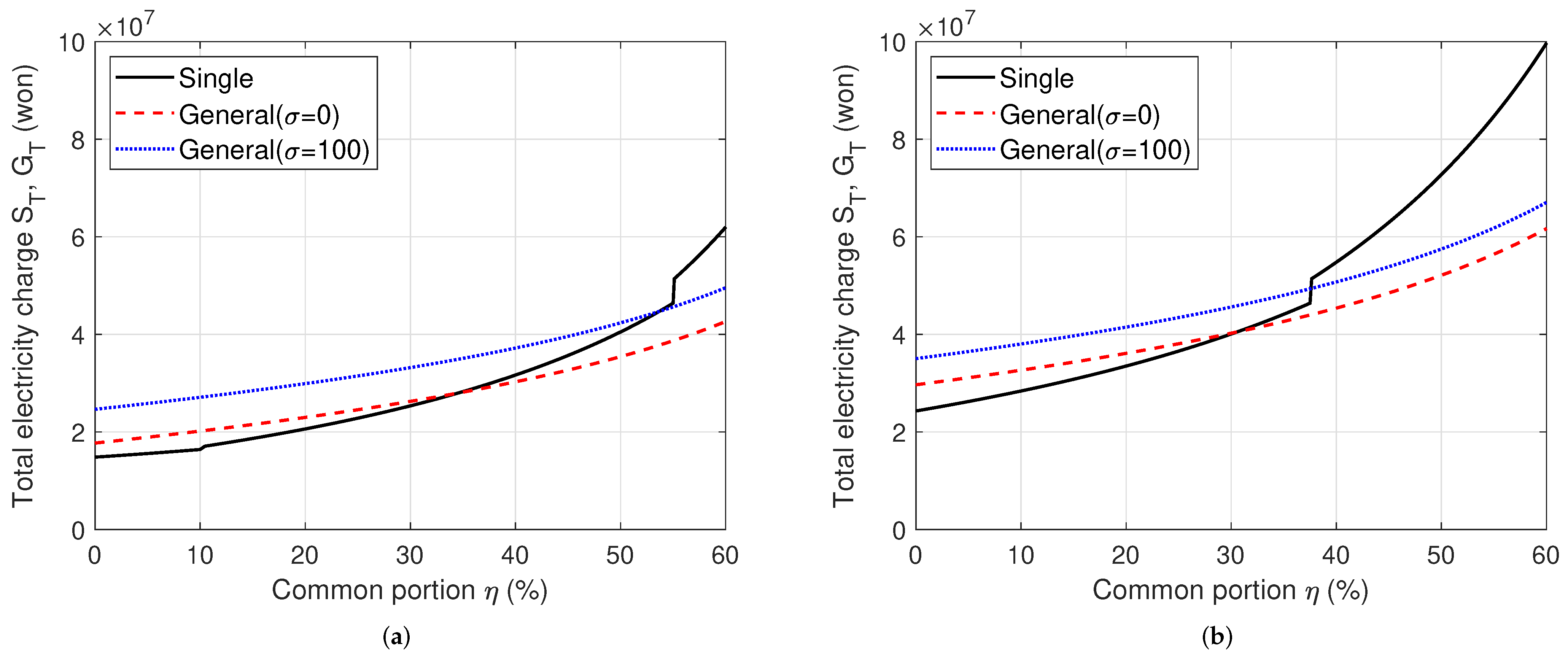
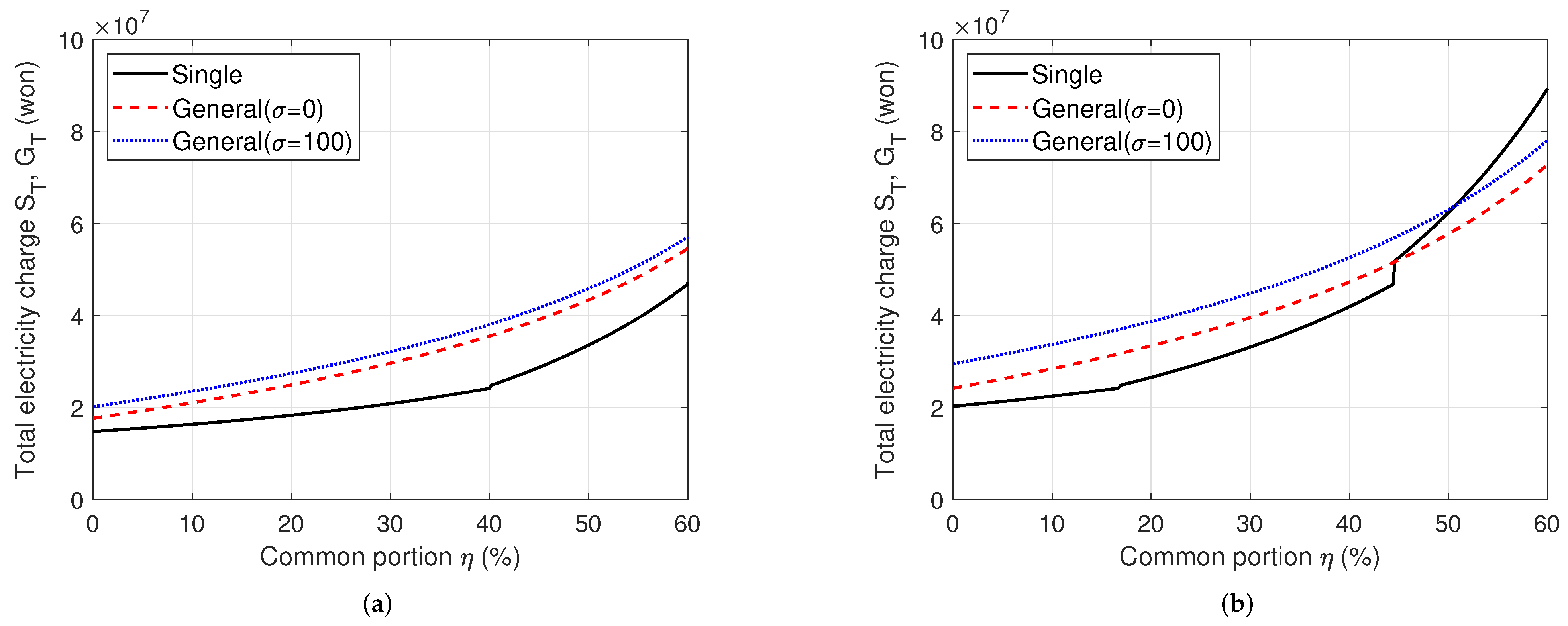
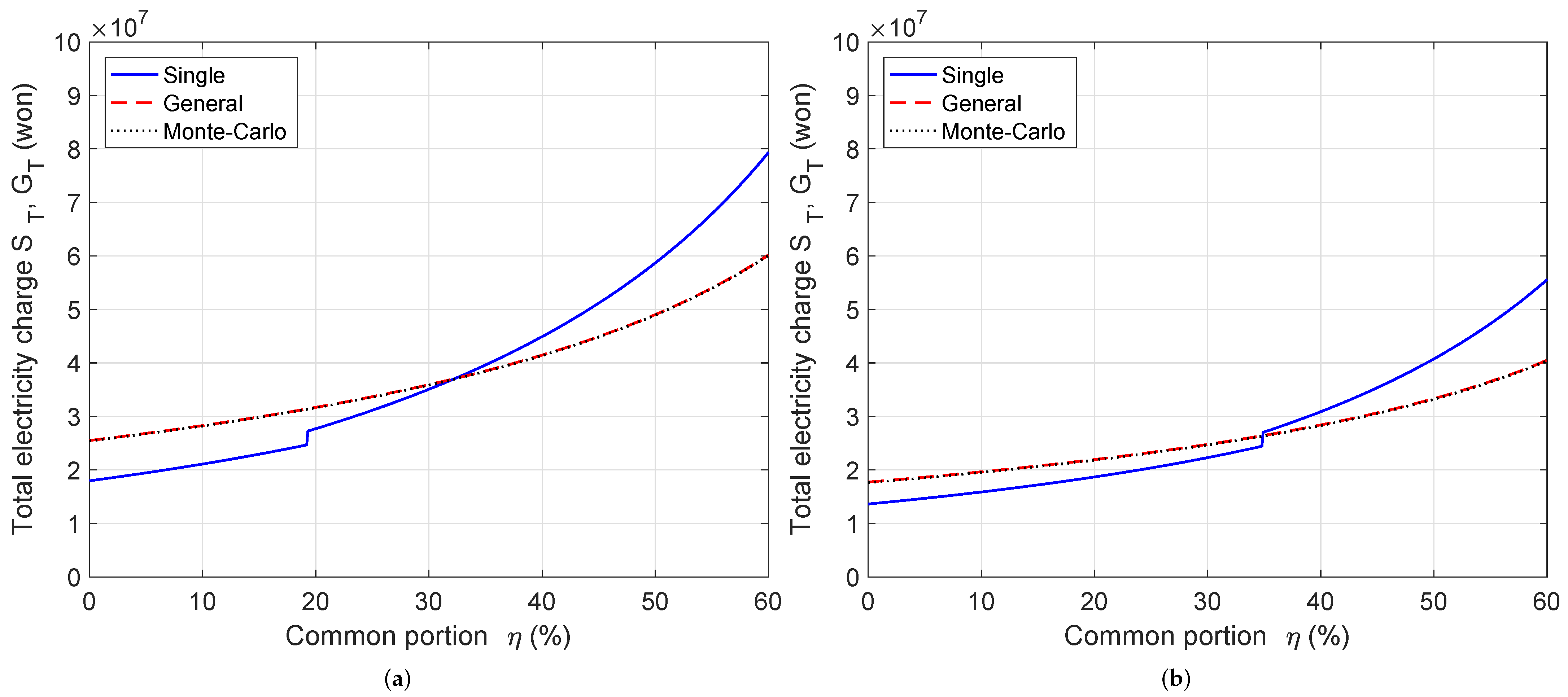
Examples of the charge curves of the single and general contracts are illustrated in Figure 4 for different $\mu =180$ kWh and 250 kWh. As shown in (13), from the start of $\eta =0$, we can observe that the charge of the single contract is lower than that of the general contract. As the common portion $\eta$ increases in Figure 4a of $\mu =180$ kWh, there is an intersection of ${\eta }_0=34.3\%$ when $\sigma =0$. After this intersection, it is clear that the general contract is more advantageous than the signal contract case. As the standard deviation $\sigma$ increases from 0 to 100, $G_T\left(\eta \right)$ also increases as shown in Figure 4a because $G_H$ of (7) increases. Hence, the intersection becomes ${\eta }_0=53.0\%$ when $\sigma =100$, which implies that the single contract is becoming more advantageous as the standard deviation $\sigma$ increases. Note that if another realization of $w_n$ satisfies the condition of the Karamata inequality [14] (p. 30), then the corresponding $G_H$ and an empirical standard deviation also increases.

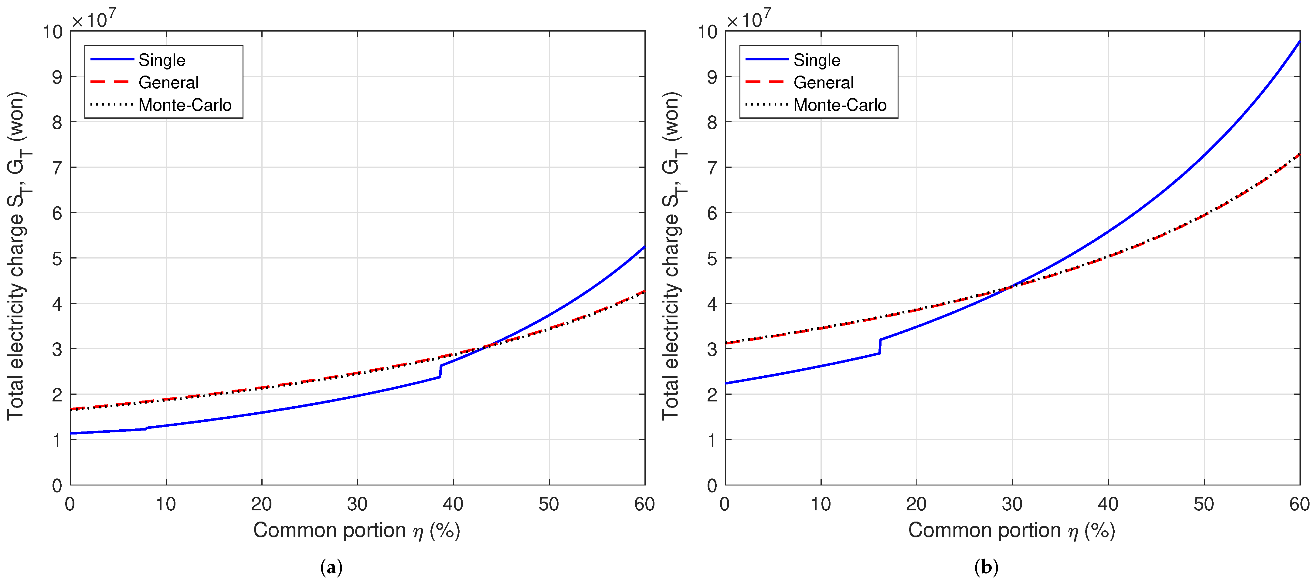
As we can observe in Figure 4, there are steps on the $S_T\left(\eta \right)$ curves of the single contract. These steps are caused by the basic rates at the range boundaries, 200 and 400 (300 and 450 for the summer season), on the rate function of $\alpha$. The positions of the steps on $S_T$ are $\eta =1-\mu /200$ and $\eta =1-\mu /400$ at the boundaries of 200 and 400, respectively. Especially at the 2nd step of 400, which is located at $\eta =1-\mu /400$ in Figure 4, the step size is larger than the 1st one of Figure 4a because of its large basic rate of 6060 won in Table 2. Note that this step can be an intersection ${\eta }_0$ for a wide range of $\mu$, $\sigma$, or $\eta$. For the summer season, the total electricity charge curves of $S_T$ and $G_T$ are illustrated in Figure 5 in a similar manner to Figure 4. We can observe that the single contract is more advantageous than the case of the other seasons of Figure 4.

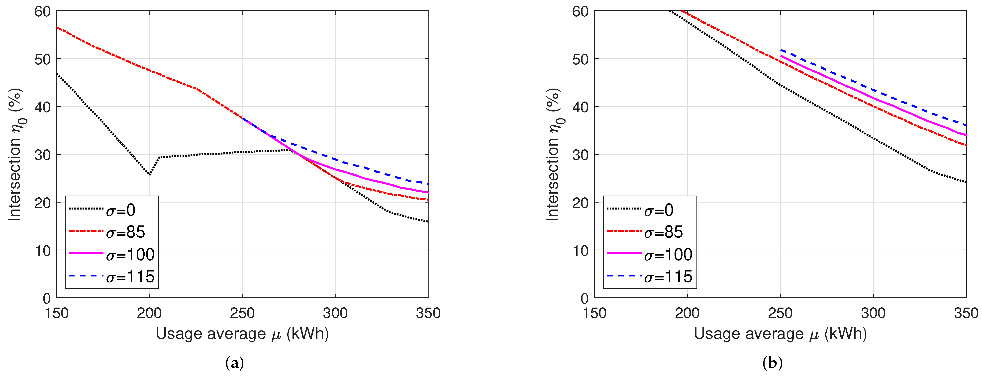
In Figure 6, curves of the intersections ${\eta }_0$ for the spring and autumn seasons are illustrated with respect to the electricity usage average $\mu$. For the cases of $\sigma =85-115$, we can observe that the ${\eta }_0$ curve decreases as the usage average $\mu$ increases. If $\sigma =0$, then $G_H$ in the general contract can be rewritten as $G_H=N·\beta \left(\mu \right)$, which shows a piecewise-linear curve as in Figure 2. The total electricity charge curve of $G_T=G_H+G_C\left(\eta \right)$ also shows a piecewise-linear curve, where $G_C\left(\eta \right)$ is an affine function for a given $\eta$. Hence, the intersections ${\eta }_0$ between the piecewise-linear functions $S_T$ and $G_T$ show a complicate curve as shown in Figure 6a for the case of $\sigma =0$. On the other hand, as $\sigma$ increases, the curve of $G_T$ becomes a smooth one and their intersections between $S_T$ also show a smooth curve except a straight line, which has a slope of $1/400$ due to the 2nd step at 400. The range of the intersections ${\eta }_0$ for usual apartment complexes is from 20 to 30. Hence, from the MC simulations of Figure 6, we notice that more than an average household electricity usage of $\mu =275$ kWh for $\sigma =100$ can provide lower electricity charges from the general contract compared to the single contract for the spring and autumn seasons. However, for the summer season, we notice that the single contract is more advantageous than the general contract case even for $\mu >350$ kWh.

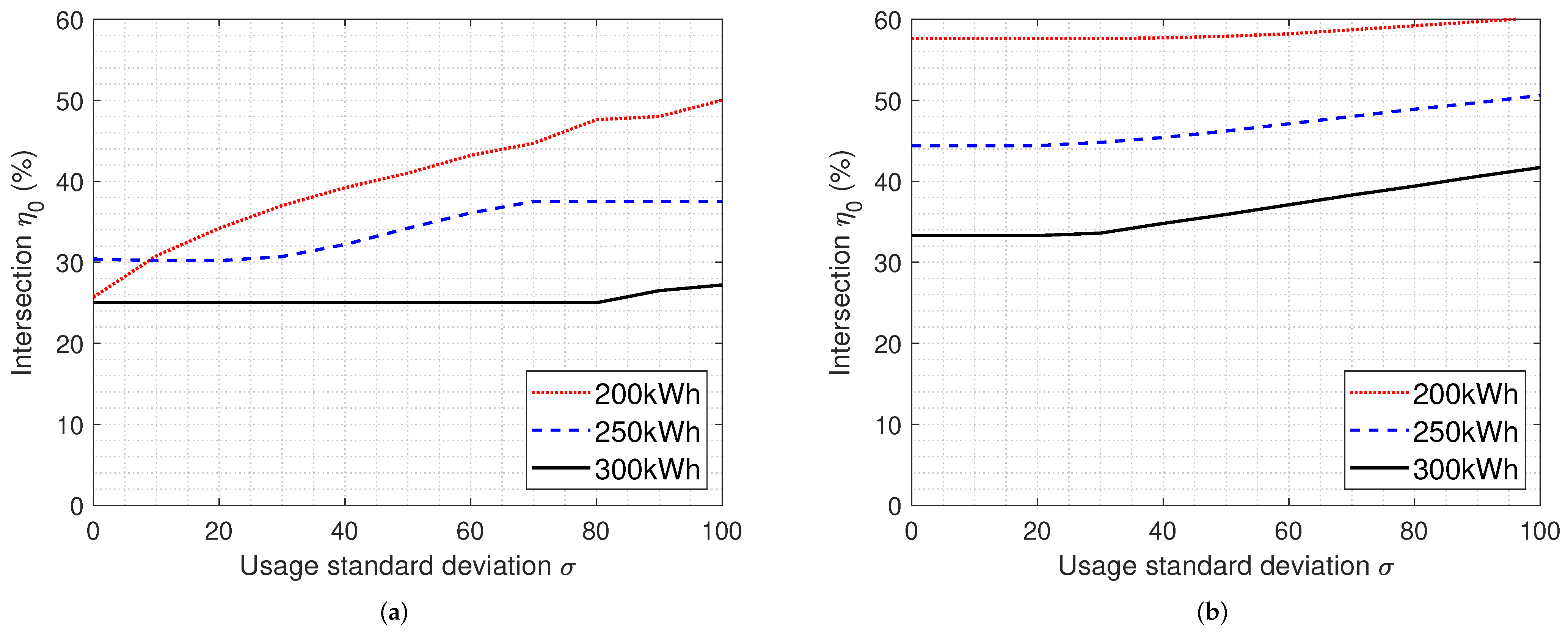
In Figure 7, curves of the intersections ${\eta }_0$ are illustrated with respect to the standard deviation of the household electricity usage. As $\sigma$ increases ${\eta }_0$ also increases because the charge curve $G_T$ increases. Hence, we notice that the single contract is getting more advantageous than the general contract case as the standard deviation of the household electricity usage increases.

5. Experimental Results

In this section, for the analyses and comparisons of the single and general contracts, we used actual metering data from 2019 to 2020 obtained from 30 apartment complexes. For each apartment complex, the average household usages on $\mu$ and standard deviations on $\sigma$ are first empirically estimated for 12 months by using metering data of $w_n$ and then their 12-month averages of the averages and standard deviations are calculated because the electricity charges are calculated on a monthly basis. The 12-month averages and standard deviations are plotted in Figure 8a. The number of households N are also plotted in Figure 8b to show sizes of the considered apartment complexes.

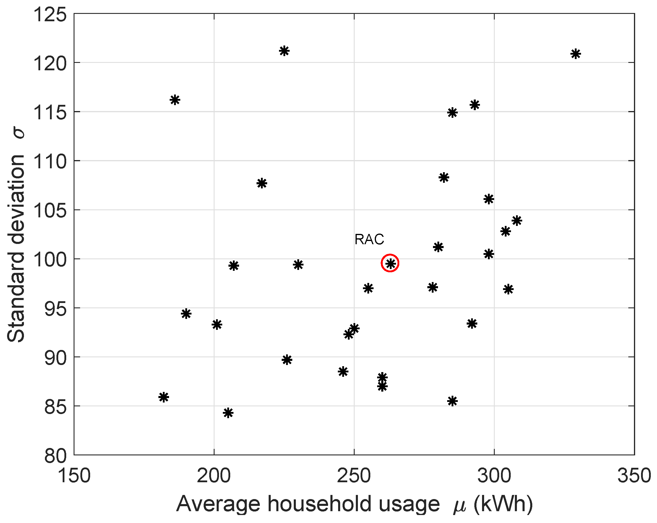
The 12-month averages of the household averages and standard deviations of the considered 30 apartment complexes are summarized in Figure 9 as a scatter diagram. The 12-month averages for $\mu$ and $\sigma$ are 258 kWh and 99.7, respectively. Among the apartment complexes, based on these 12-month averages, we selected a representative apartment complex (RAC), in which $\mu \approx 261$ kWh and $\sigma \approx 96.1$, respectively. Here, the RAC, which is the fourth one in Figure 8 and is indicated as a red circle in Figure 9, has 527 households and the contract power is $W_{CP}=1700$ won. From Figure 9, it seems that the averages and standard deviations have no correlations with each other. In other words, the apartment complex, which consumes small electrical energy, can have a large standard deviation of the household usages.

For the RAC of the 30 apartment complexes, examples of the electricity charge curves of $S_T$ and $G_T$ are illustrated with the results of the MC simulations in Figure 10. We can observe that the MC simulation results, which are based on a model with normal distributions, faithfully follow the charge curve of the general contract $G_T$. For the August case of Figure 10a, the intersection is ${\eta }_0=32.2$. The MC simulation yields an intersection of ${\eta }_{MC}=32.0$. For the December case of Figure 10b, the intersection increases to the 2nd step on $S_T$ as ${\eta }_0=34.8$. The MC simulation yields the same intersection of ${\eta }_{MC}=34.8$ due to the 2nd step on $S_T$ at the 2nd threshold of 400. Compared to the August result of Figure 10a, in Figure 11, other examples are shown for the 2nd and 20th apartment complexes in August. The case of Figure 11a has a similar standard deviation to the RAC case of Figure 10a, however has lower average household usage on $\mu$. As observed in Figure 6, the 2nd apartment complex of Figure 11a shows a higher intersection. For the case of Figure 11b, the average and standard deviation are similar to those of the RAC case of Figure 10a. Hence, their intersections are similar to each other.

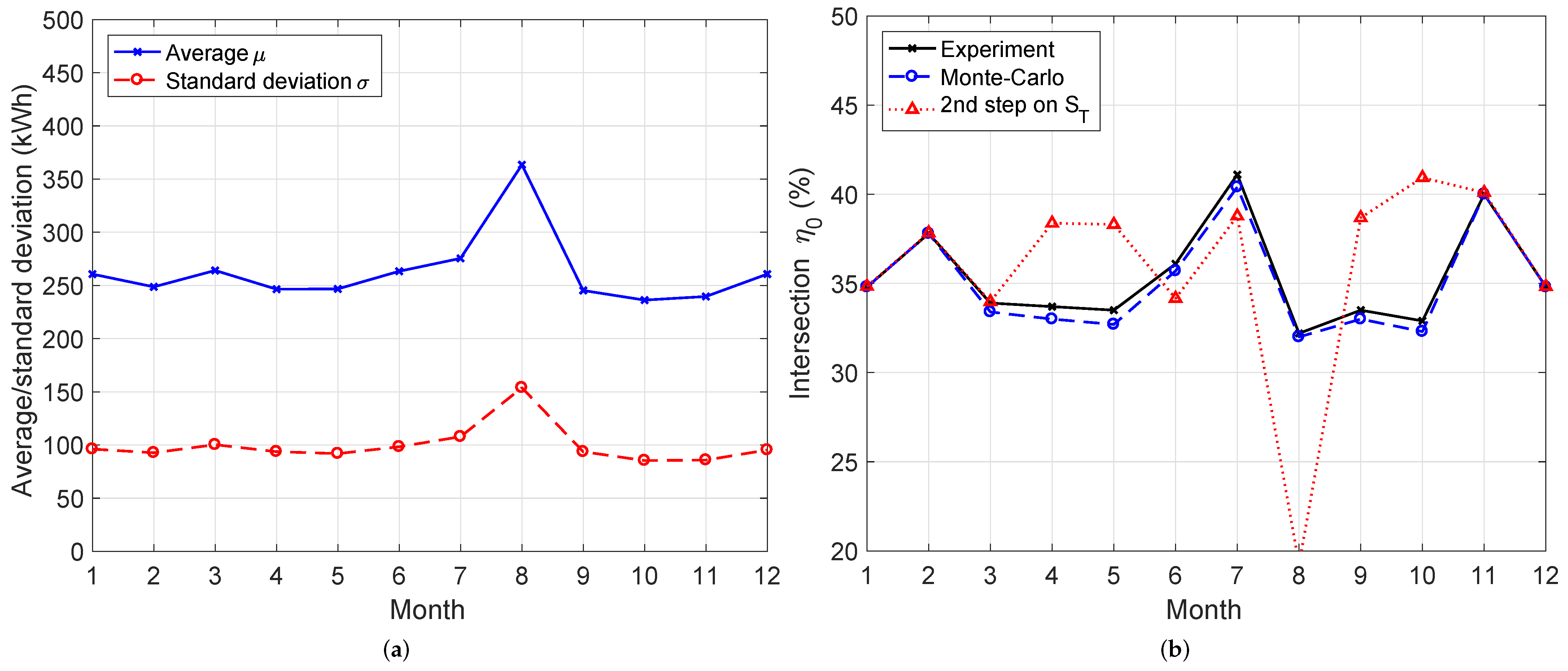
In Figure 12a, for the RAC, the averages and standard deviations with respect to month are plotted to show trends of electricity usages. In Figure 12b, experimental results for the RAC and their MC simulations are compared. In the MC simulations based on the proposed model, only the average of $\mu$ and standard deviation of $\sigma$ for different months were used to estimate the intersections ${\eta }_0$ with a small mean square error (MSE) of 0.2233. Here, the MSE, which is a 12-month average, is defined as

$$\begin{array}{c}\hfill \mathrm{MSE}:=\frac{1}{12}\sum _{k=1}^{12}{\left[{\eta }_0\left(k\right)-{\eta }_{MC}\left(k\right)\right]}^2,\end{array}$$

(14)

where ${\eta }_{MC}\left(k\right)$ is the intersection estimate from the MC simulation based on the proposed model for the kth month. We can observe that the intersections estimated based on the proposed model can successfully provide the true intersections for a given apartment complex. In other words, without personal information, such as the household electricity usage of $w_n$, we can estimate the intersection ${\eta }_0$ using only their average and standard deviation of Figure 12a for a given $N=527$. Therefore, the proposed model can support a simple diagnostic method whether the single or general contract is advantageous or not for a given apartment complex. The positions of the 2nd steps on $S_T$ are also plotted in Figure 12b. We notice that for the winter season and March, the intersections are equal to the step positions and thus the estimates from the MC simulations are equal to those of the true intersections. In the generic high-voltage rate of Table 3, because the rates in the spring and autumn seasons are lowest among those of other seasons, the total electricity charge of the general contract decreases and yields relatively low intersections as shown in Figure 12b. Hence, we can consider a seasonal contract, in which only for the spring and autumn seasons, the electricity charge of the general contract is applied [13].

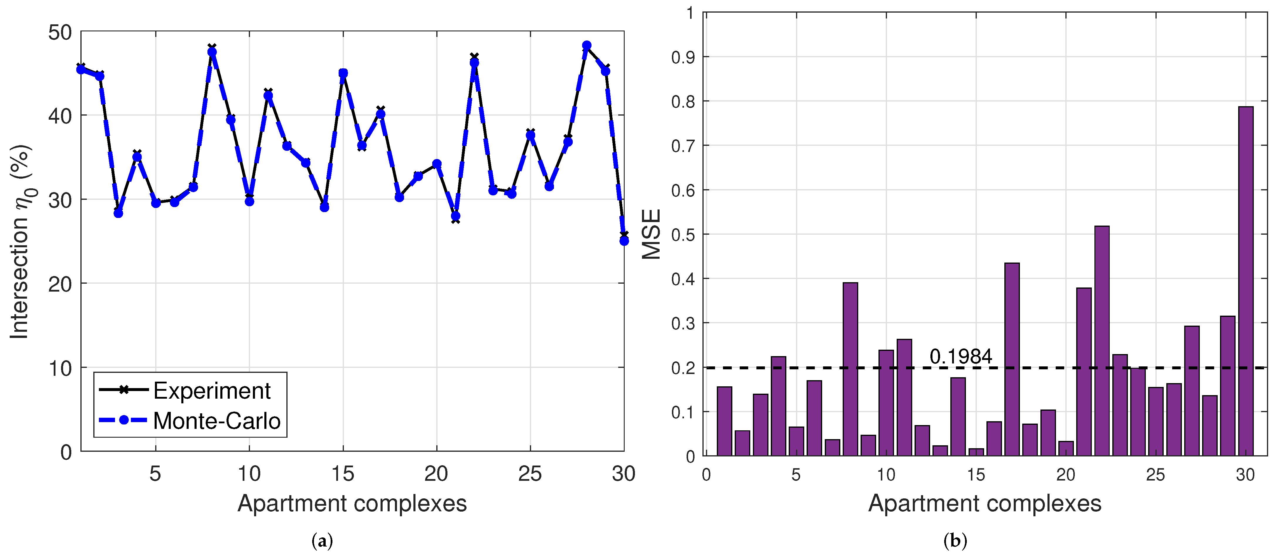
In Figure 13a, the intersections of ${\eta }_0$ from the experiments and the MC simulations are illustrated for each apartment complex. The average over the 30 apartment complexes of the experimental intersections is 36.2 and most of the intersections are greater than 28, which means that the single contract is advantageous in most cases. In Figure 13b, the MSE of the intersection estimates from the MC simulations for the considered 30 apartment complexes are summarized. We can observe that the MC simulations can successfully estimate the intersections, which can provide good guidelines in analyzing the advantages of the single and general contracts for a given apartment complex without knowing personal information of $w_n$.

6. Conclusions

In this paper, the single and general contracts, which are employed for the medium-voltage apartment complexes in the Republic of Korea, are analyzed and compared based on both MC simulations and actual metering data from 30 apartment complexes. Properties of the single and general contracts are comparatively summarized in

Table 4. Comparison of the current single and general contracts for the medium-voltage apartment complexes in the Republic of Korea.

		Single Contract	General Contract
Rate	Household usage ${\mathit{W}}_{\mathit{H}}$	Residential high-voltage (Table 2)	Residential low-voltage (Table 1)
	Common usage ${\mathit{W}}_{\mathit{C}}$		Generic high-voltage (Table 3)
Total electricity charge		$S_T\left(\eta \right)=N·\alpha (W_H/N(1-\eta ))$	$G_T\left(\eta \right)=G_C\left(\eta \right)+G_H$
Features		- Simple calculation	- Independent electricity charge
		- Independence of $\sigma$	- No steps on the $G_T$ curve
		- Steep slope of $S_T\left(\eta \right)$ as $\eta$ increases	- No progressive rate for $G_C$
Preference		- For low common portions of $\eta$	- For high common portions of $\eta$
		- For high $\sigma$	- For high $\mu \approx W_H/N$
		- For summer and winter	- For spring and autumn
Problems		- Progressive rate for $W_C$	- $G_T$ increases as $\sigma$ increases
		- Steps on the $S_T$ curve	- High $G_C\left(\eta \right)$ and $G_H$
		- Electricity charge dependency

. The single contract has a simple calculation scheme by using a reading data from a meter connected to the apartment complex. However, the electricity charges, which are imposed on each household, are dependent on each other and thus can be unfair depending on the amount of electricity usage. On the other hand, the general contract separately calculates the electricity charge for the household and the common usages, in which a non-progressive rate plan is applied to the common usage. Furthermore, the general contract can provide a fair independent electricity charges even though the total electricity charge of the apartment complex is larger than that of the single contract. Hence, depending on various conditions and demands in the apartment complex, the apartment complex can choose an appropriate contract method. In terms of minimizing the total electricity charge, selecting the general contract is advantageous for apartment complexes that use relatively large electrical energy. From the analysis, it is also shown that the current electricity rates, which are employed in the single and general contracts, provide an unbalanced electricity charges to the apartment complexes. The MC simulation can provide a method to find a balanced electricity charge by modifying the electricity rates and can be useful in developing a new electricity charging system.