Highly Accurate Experimental Heave Decay Tests with a Floating Sphere: A Public Benchmark Dataset for Model Validation of Fluid–Structure Interaction

 ,
,  ,
,  ,
,  , , ,
, , , 
 , ,
, , 
 ,
, 
Abstract
1. Introduction
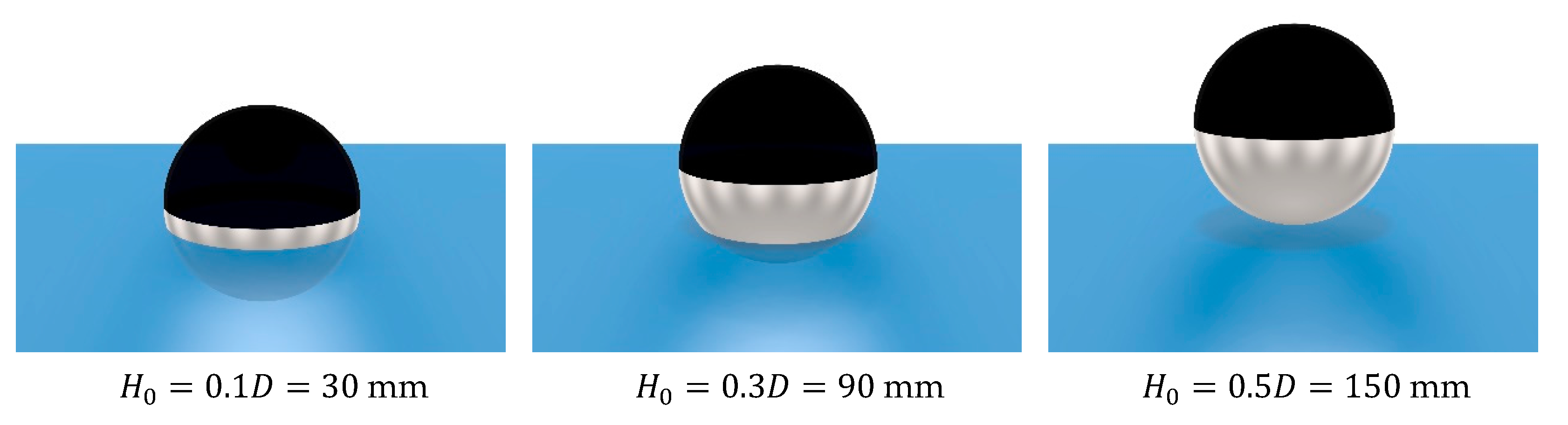
1.1. The Test Case
1.2. Numerical Modelling Blind Tests of the Test Case
1.3. RANS Models
1.4. FNPF Models
1.5. LPF Models
2. Materials and Experimental Setup
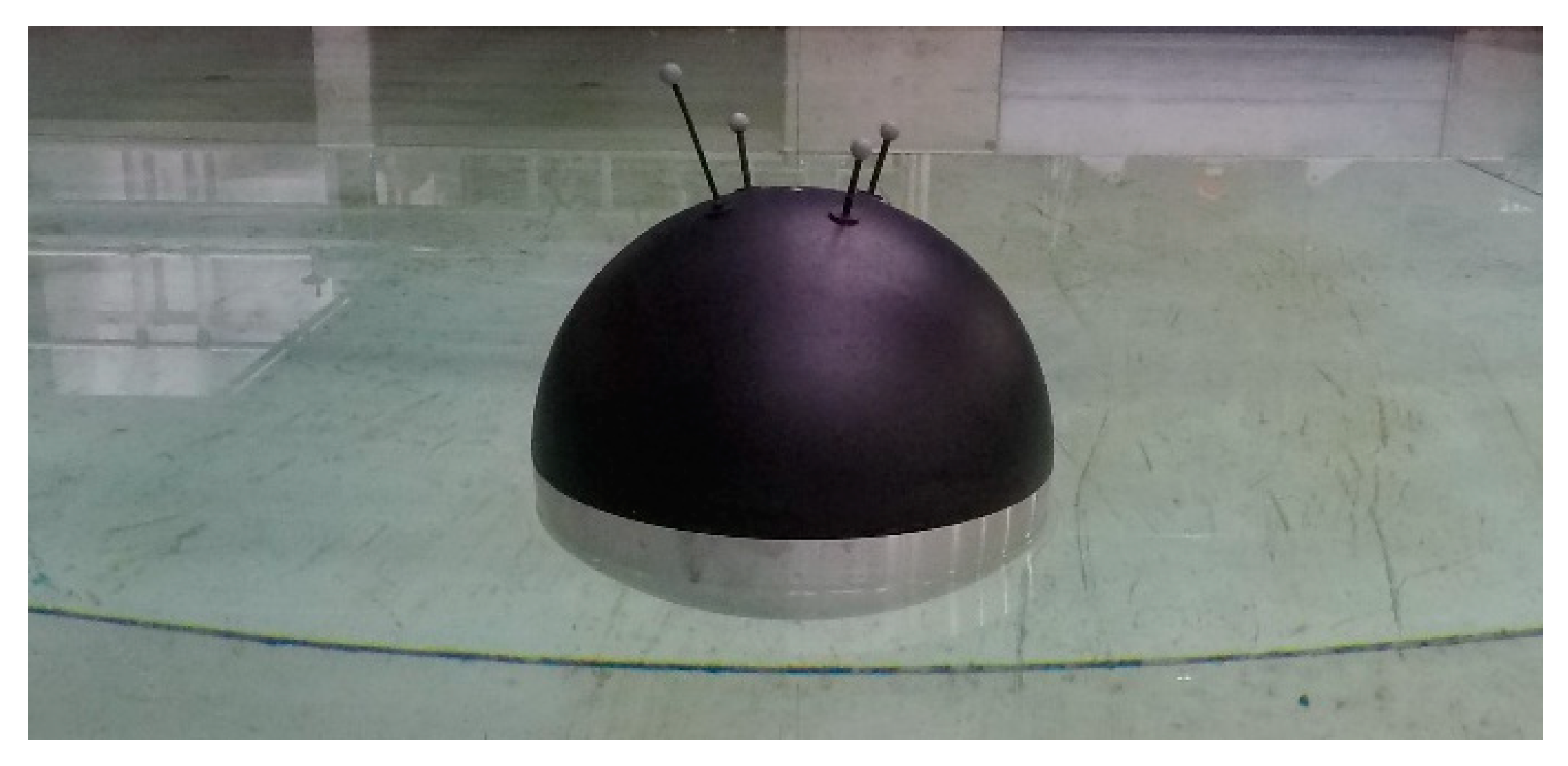
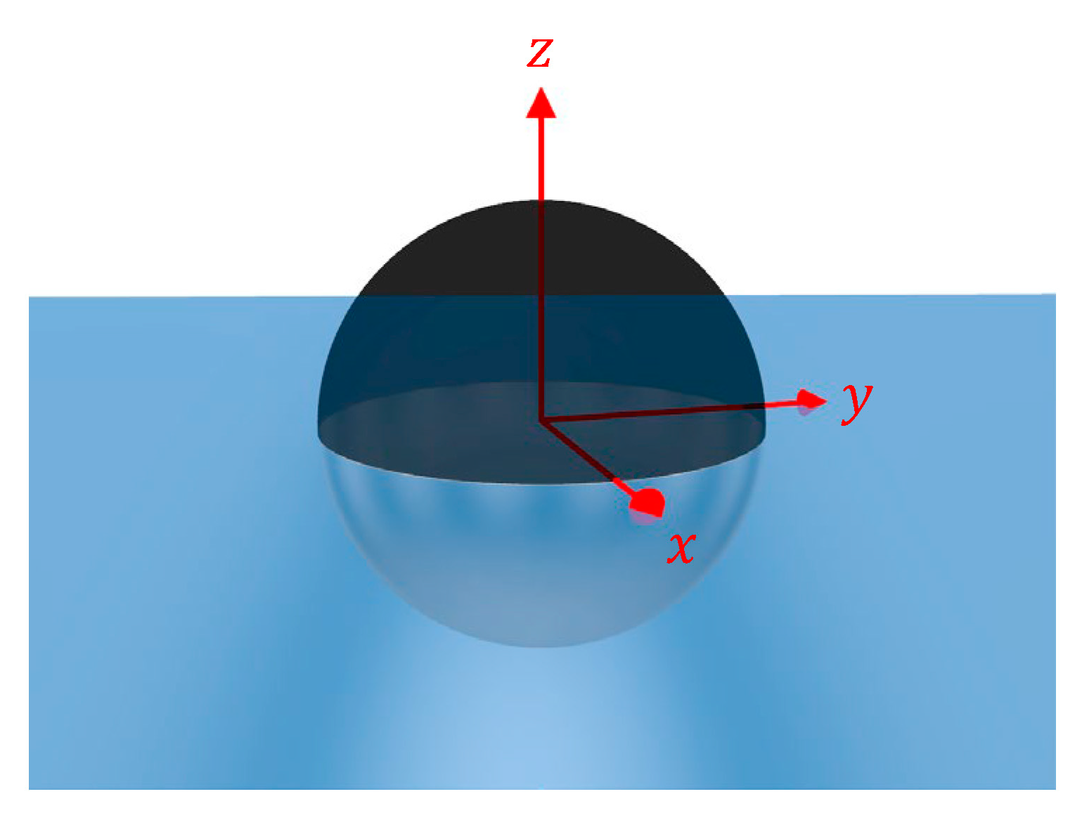
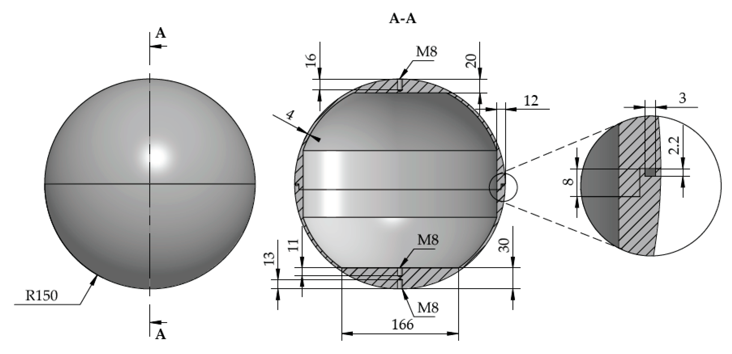
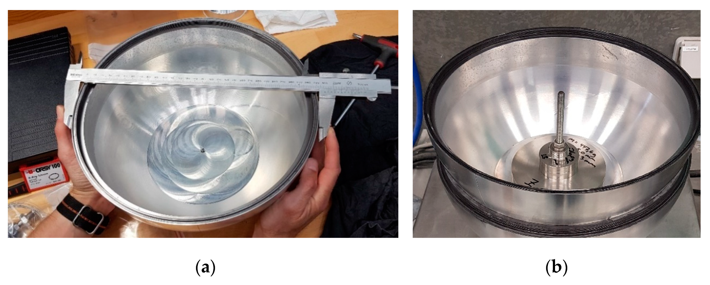
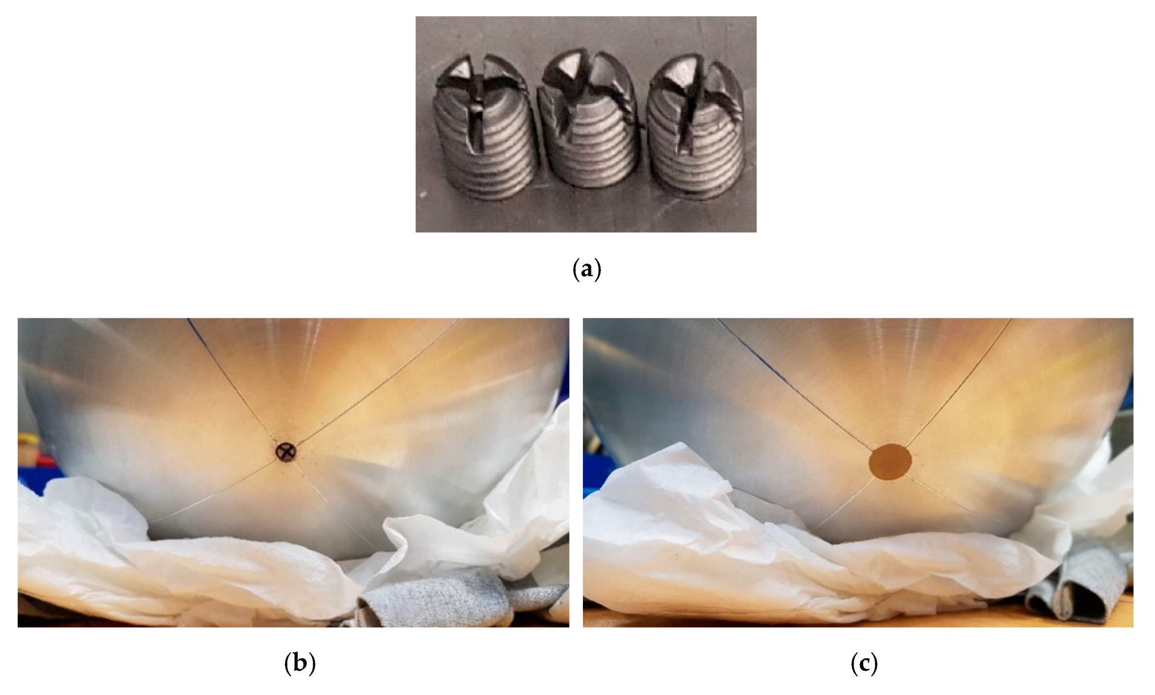
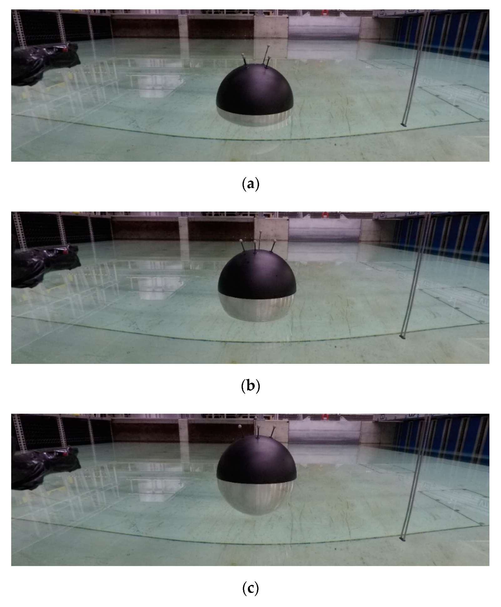
2.1. The Sphere Model
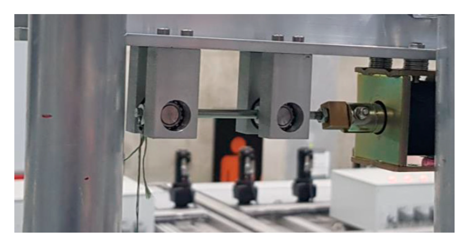
2.2. Experimental Setup and Equipment
3. Results
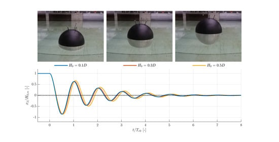
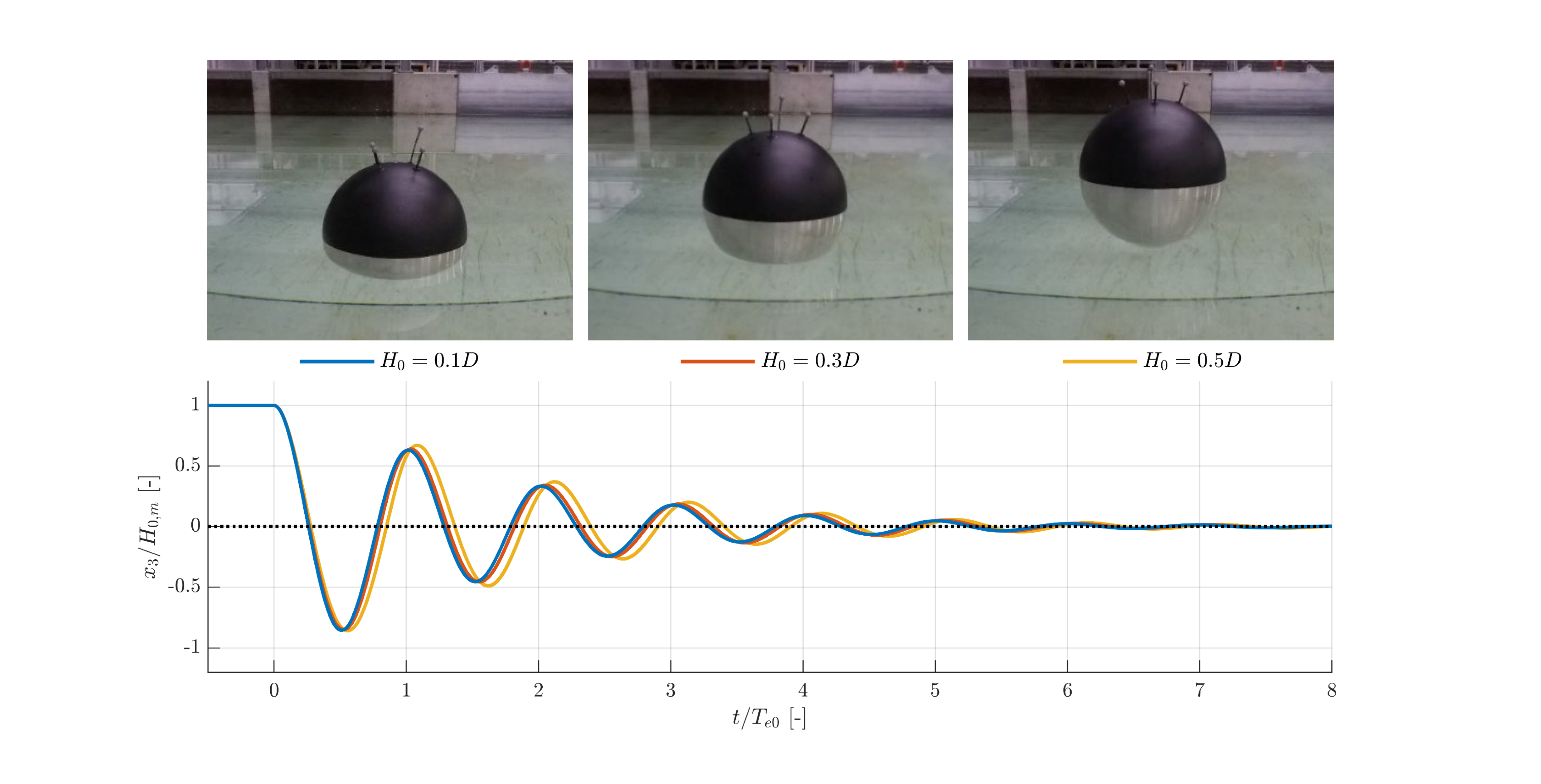
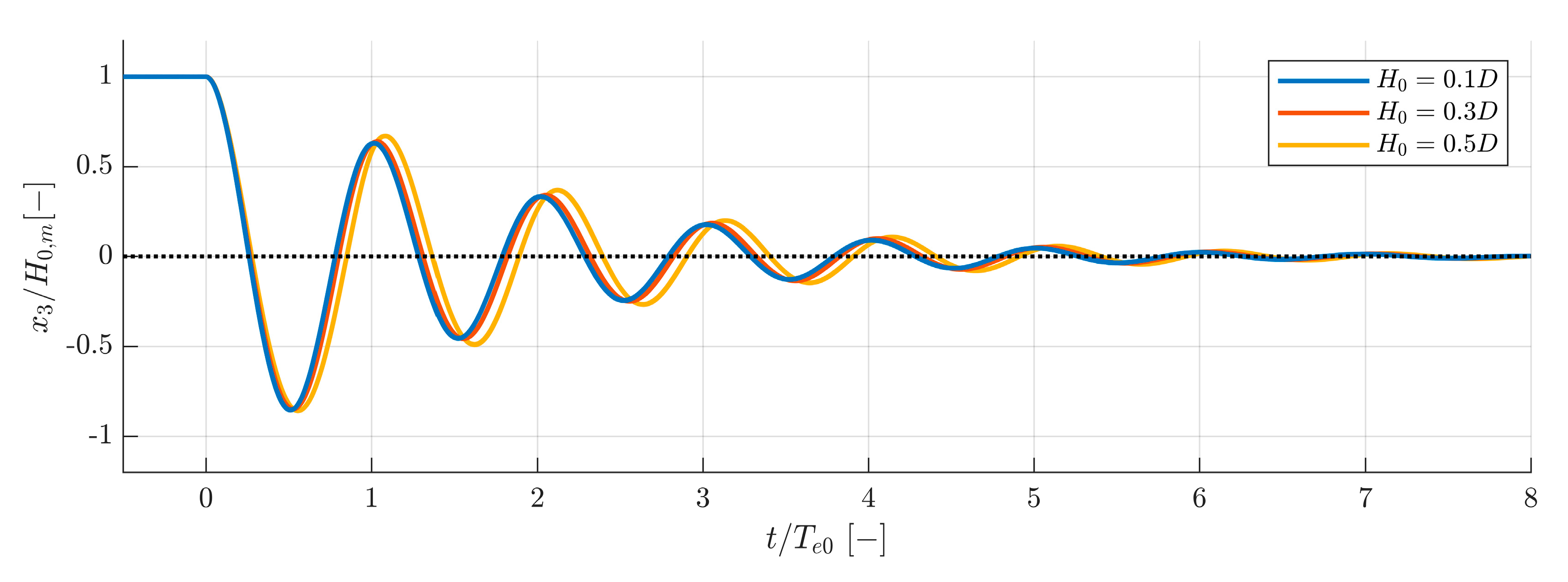
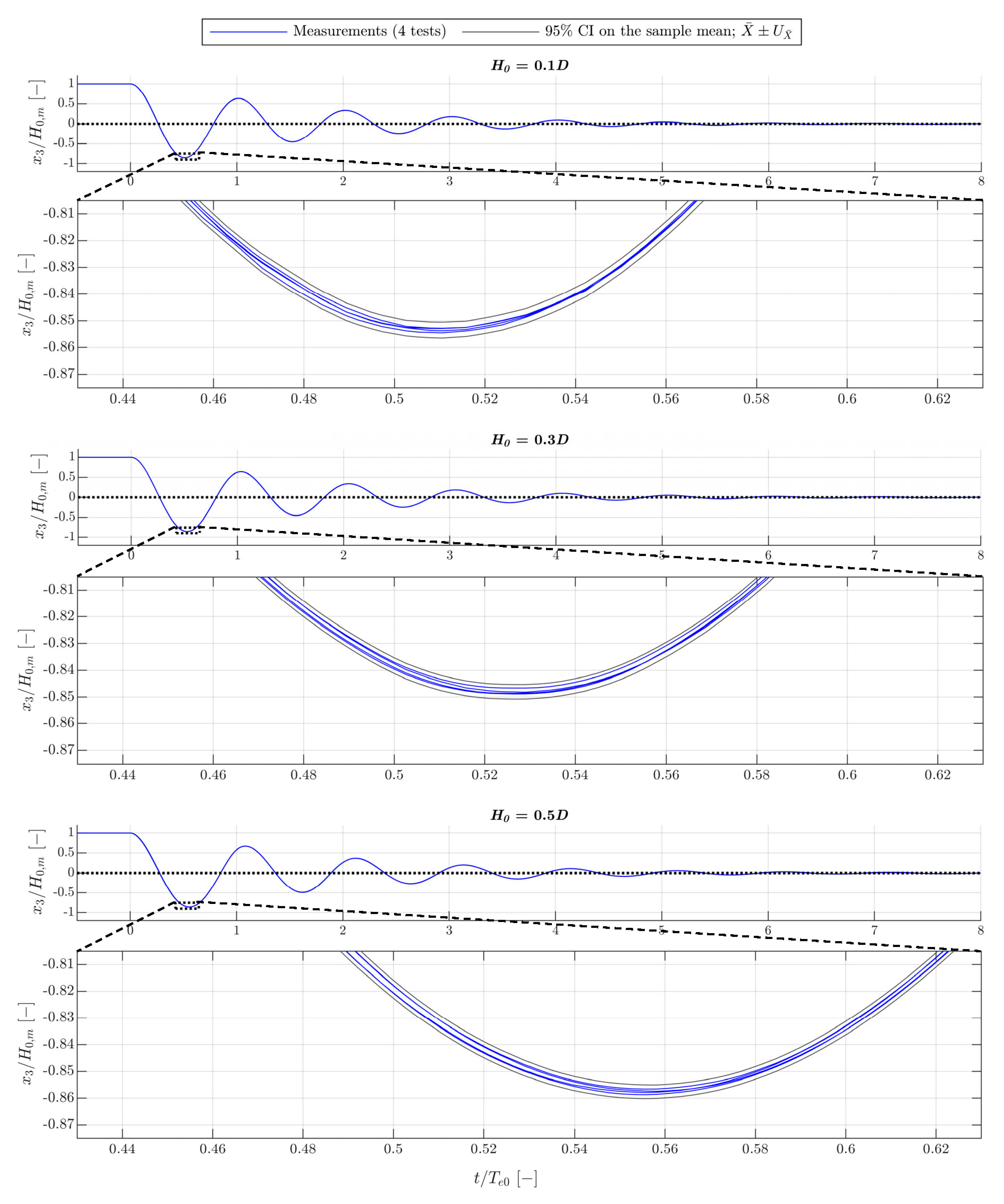
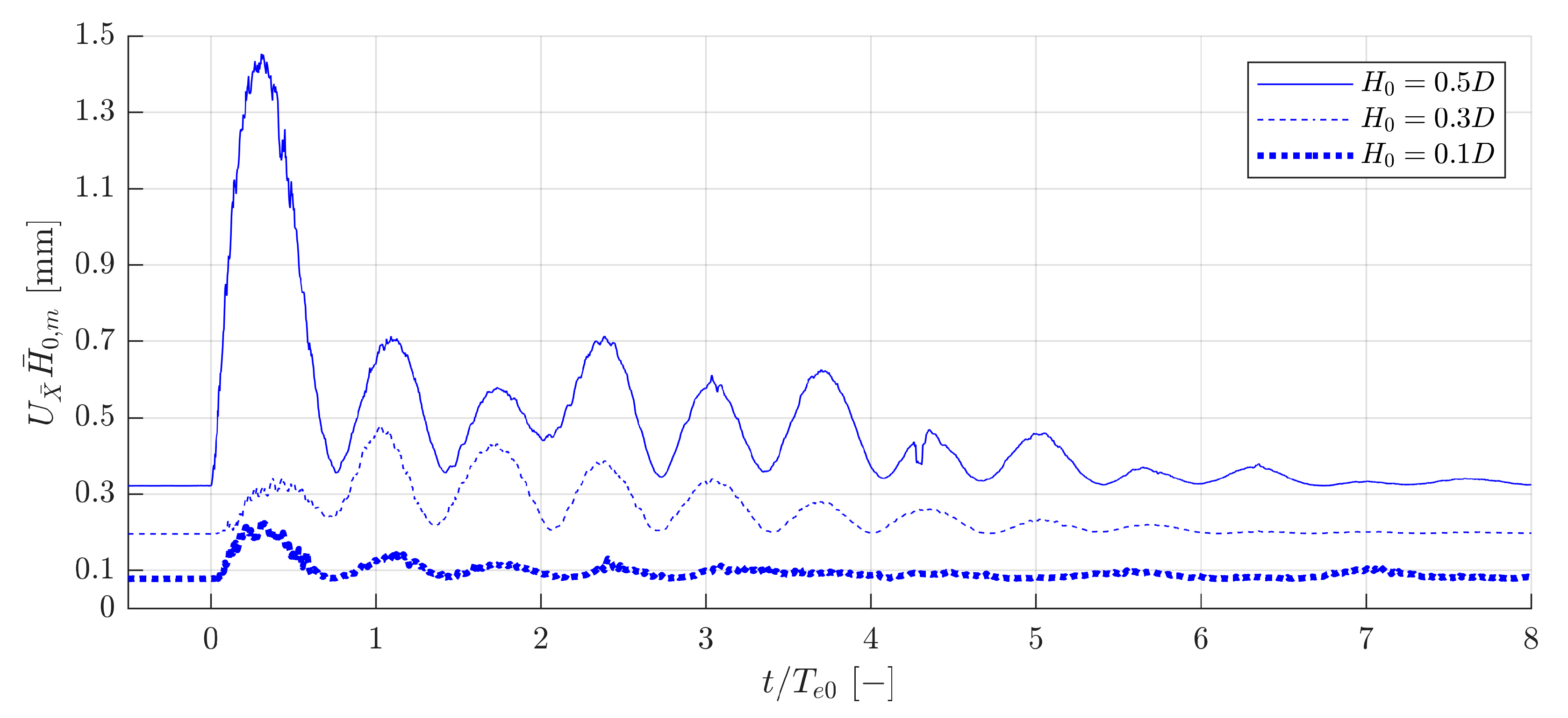
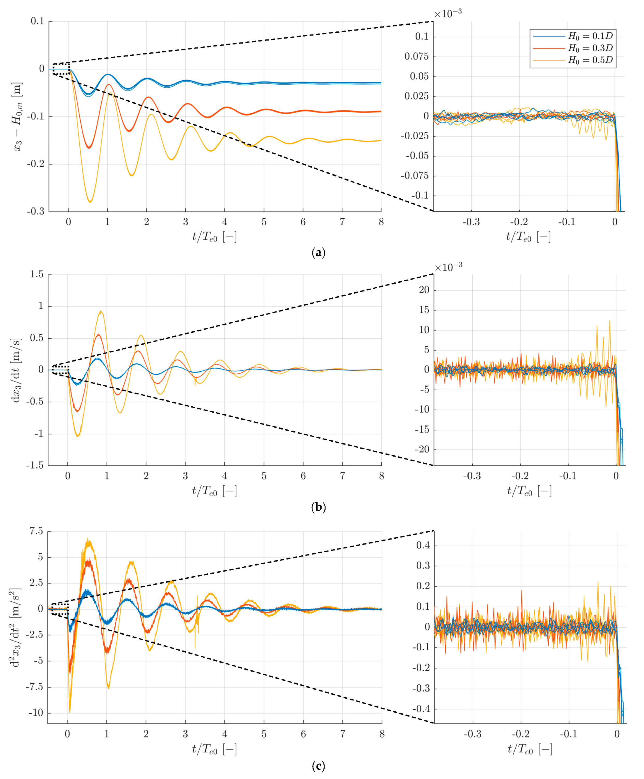
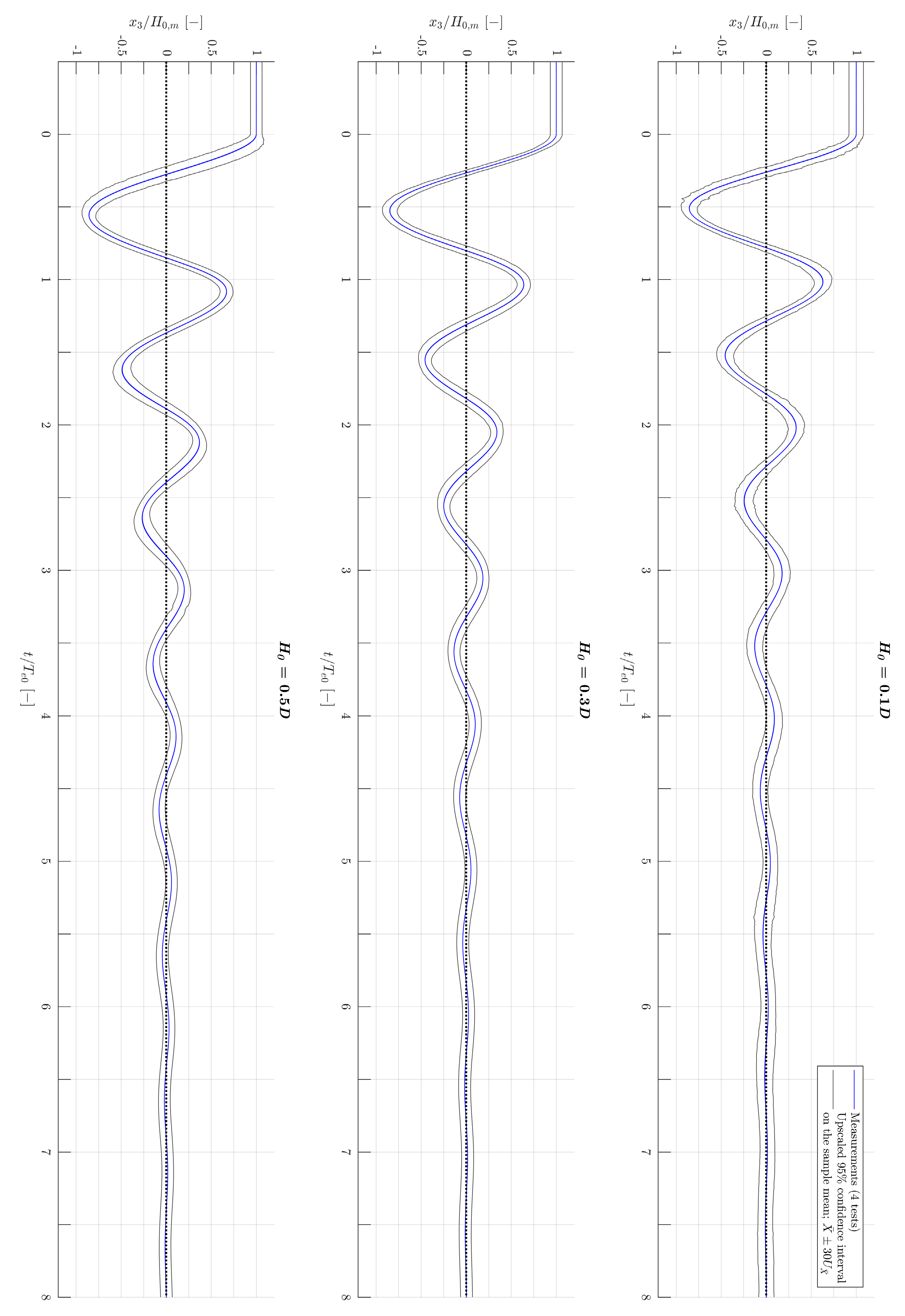
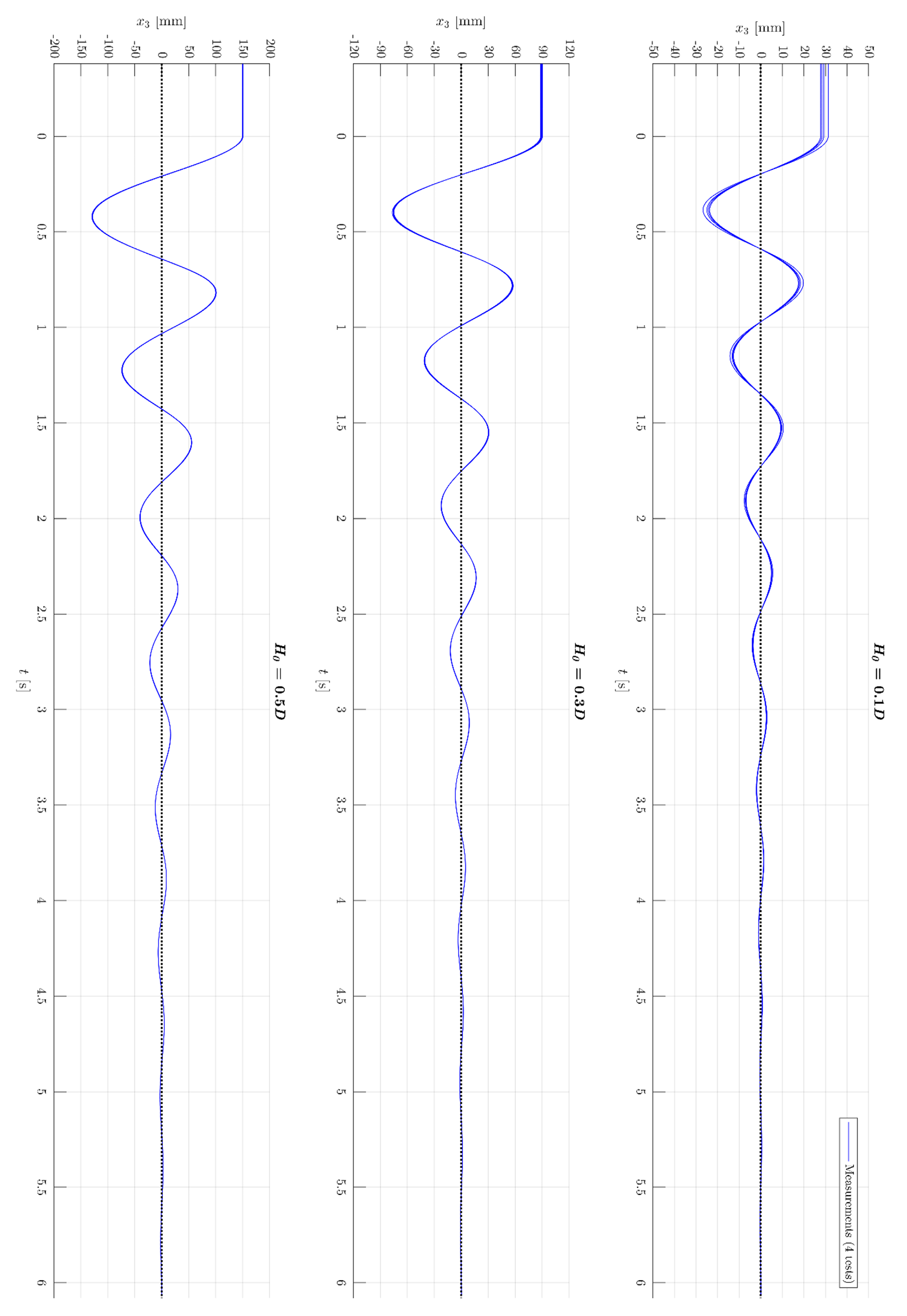
3.1. Decay Measurements and Expanded Uncertainty
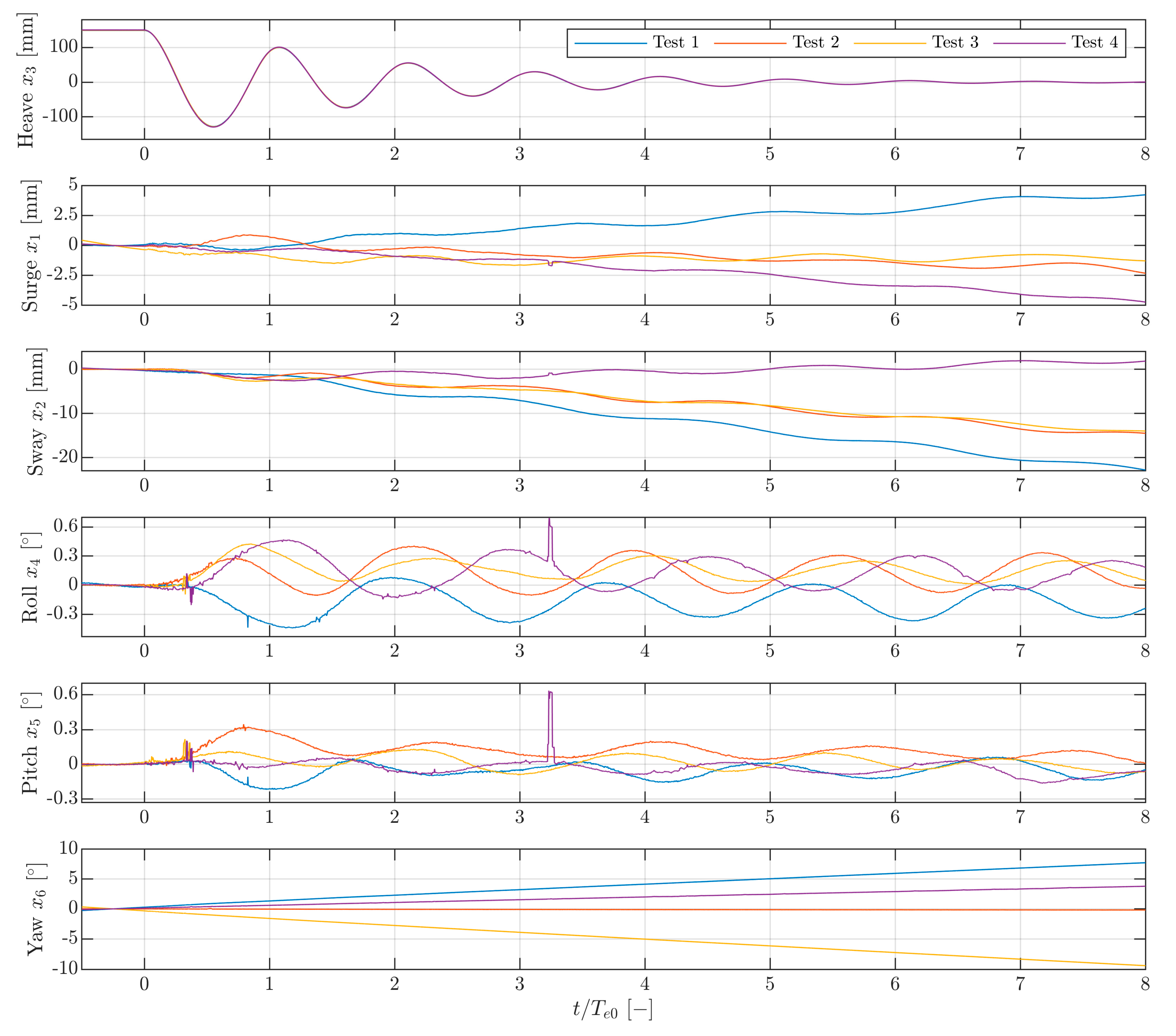
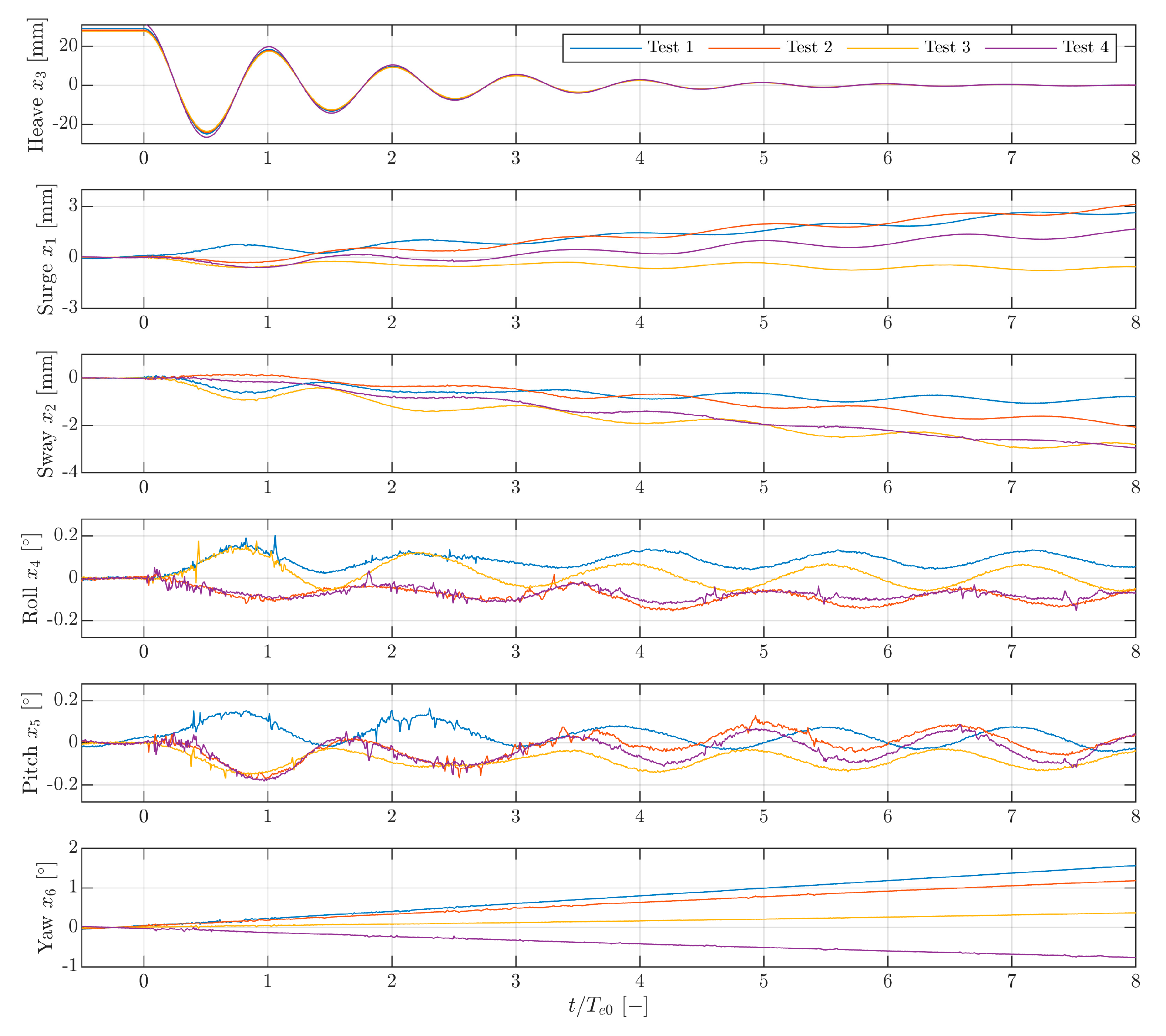
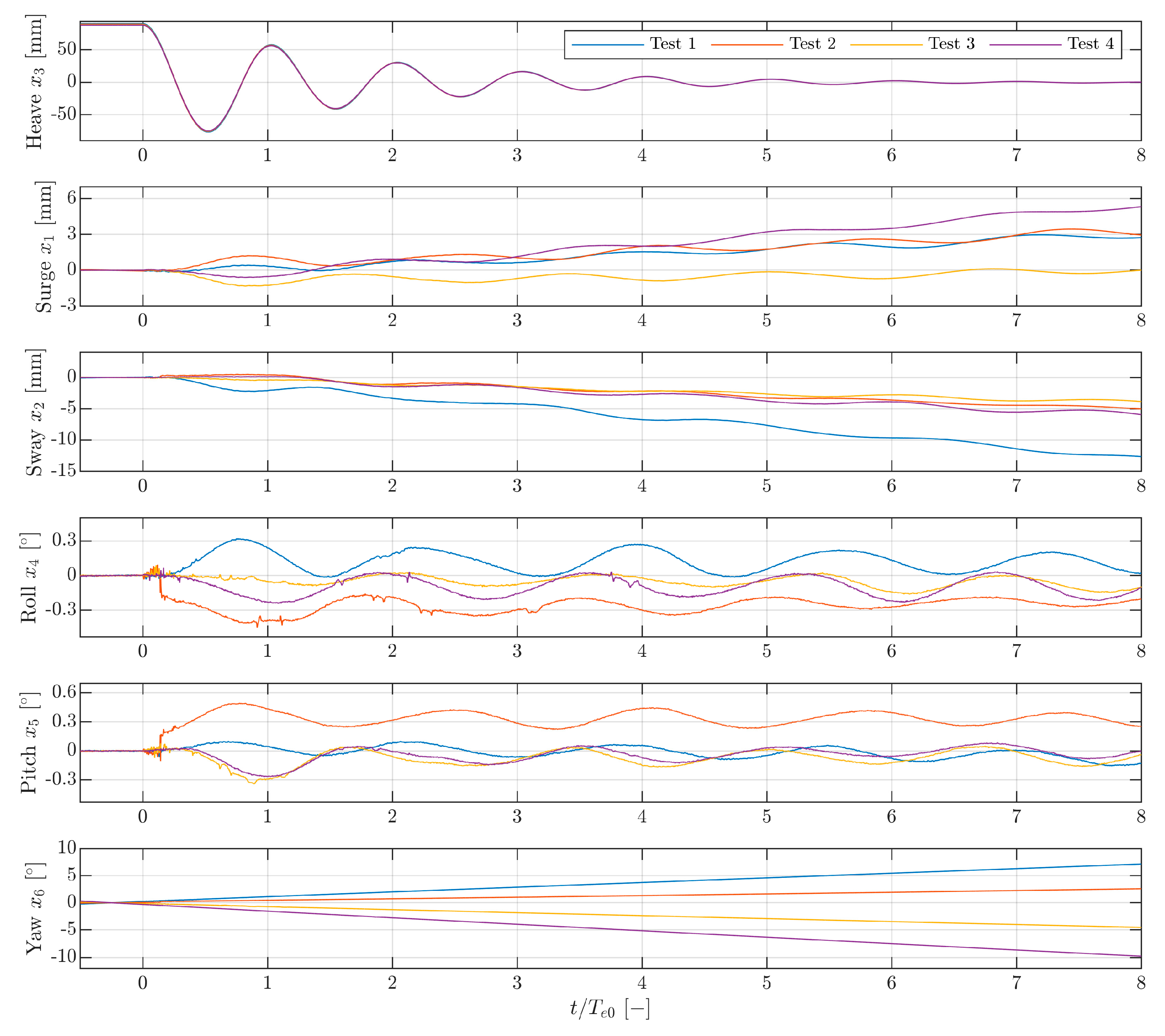
3.2. Six DoF Motions
3.3. Initial Calmness of the Sphere Model
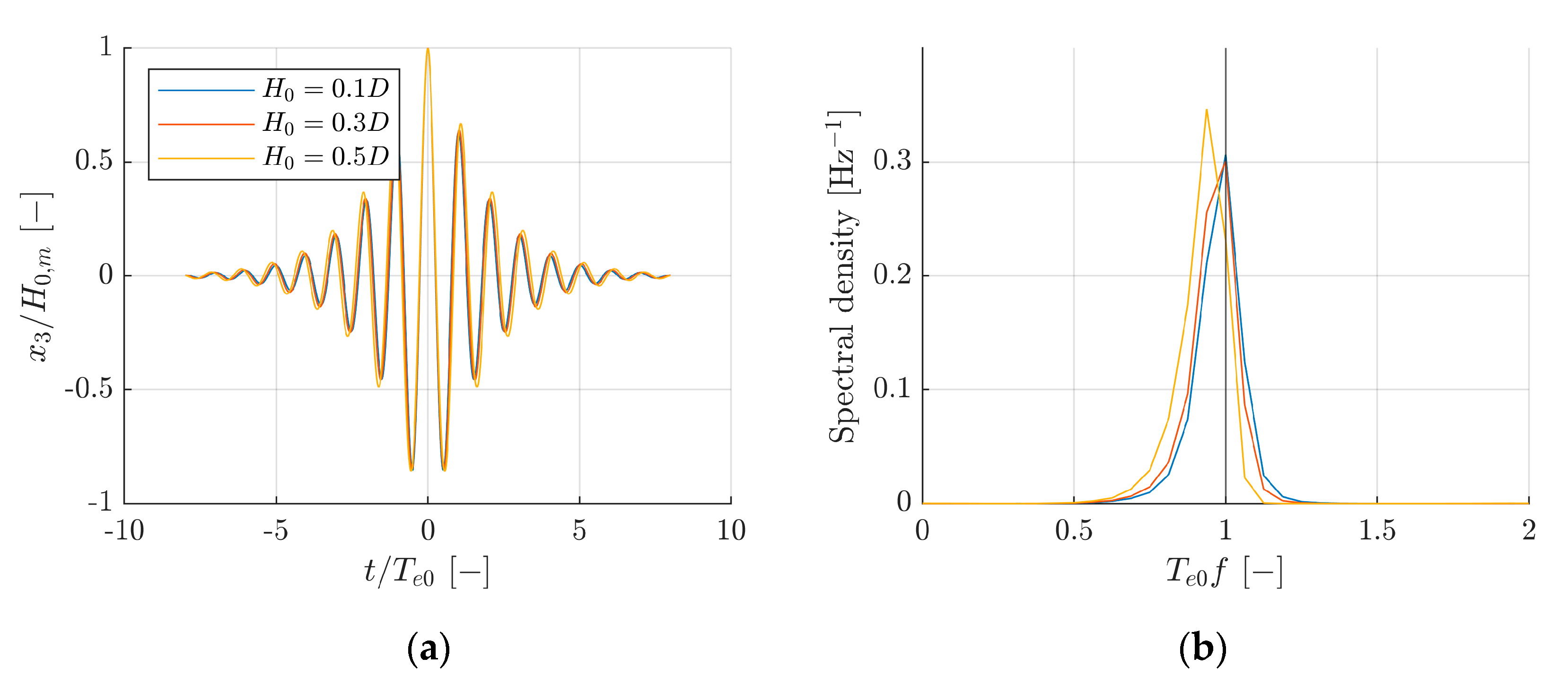
3.4. Frequency Content
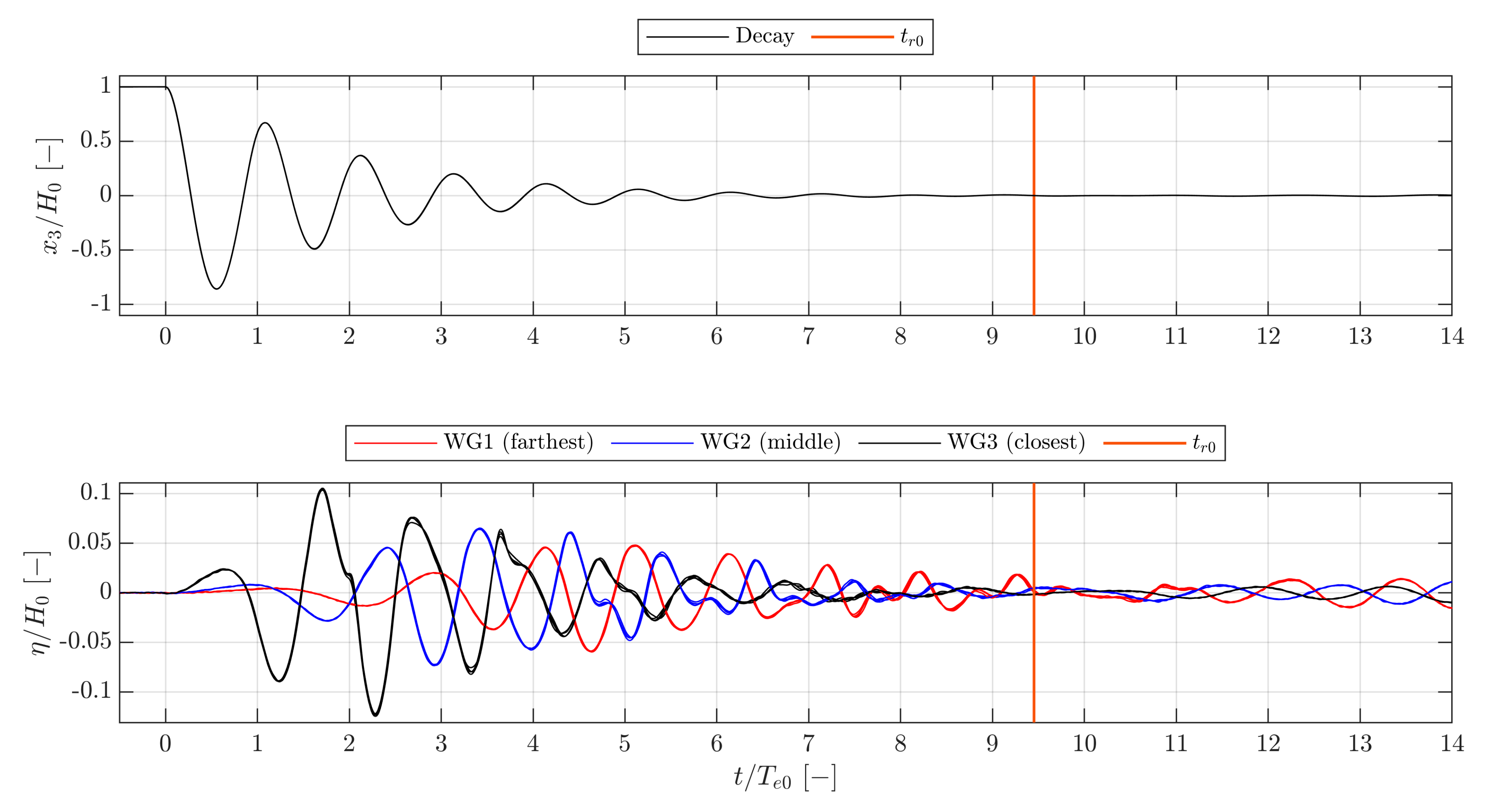
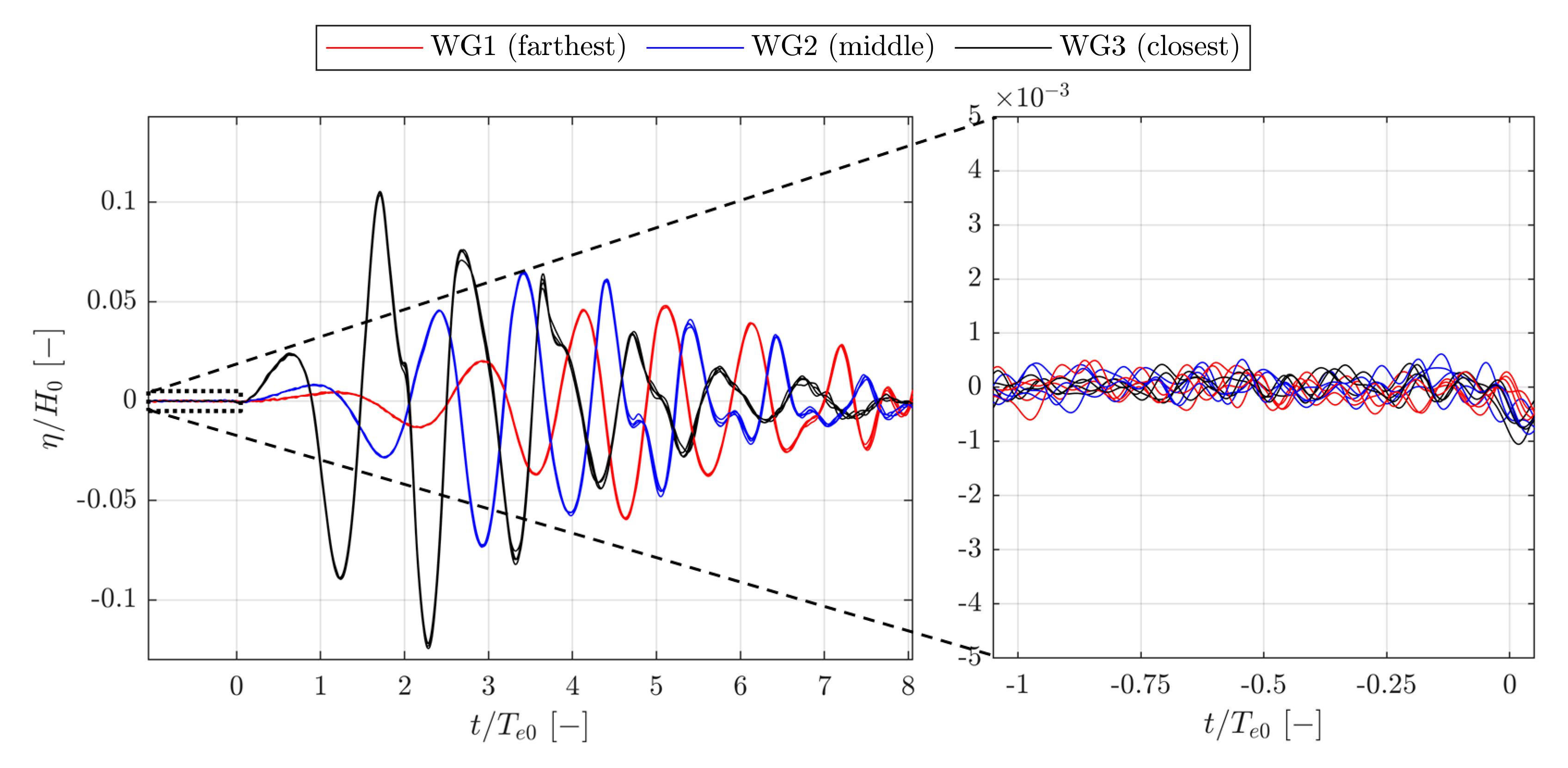
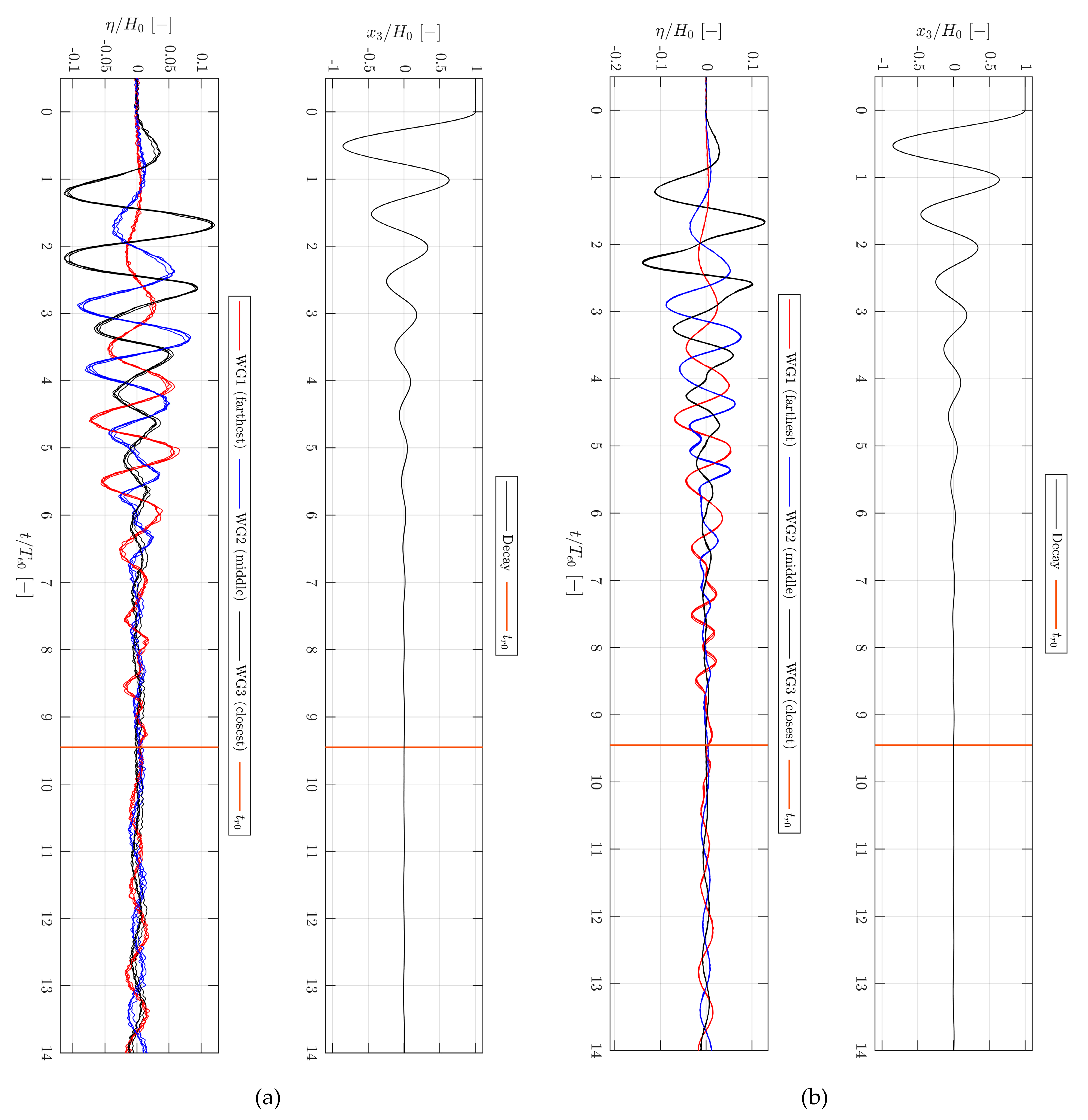
3.5. Reflections and Initial Calmness of the Water Phase
3.6. Uncertainties of Physical Parameters
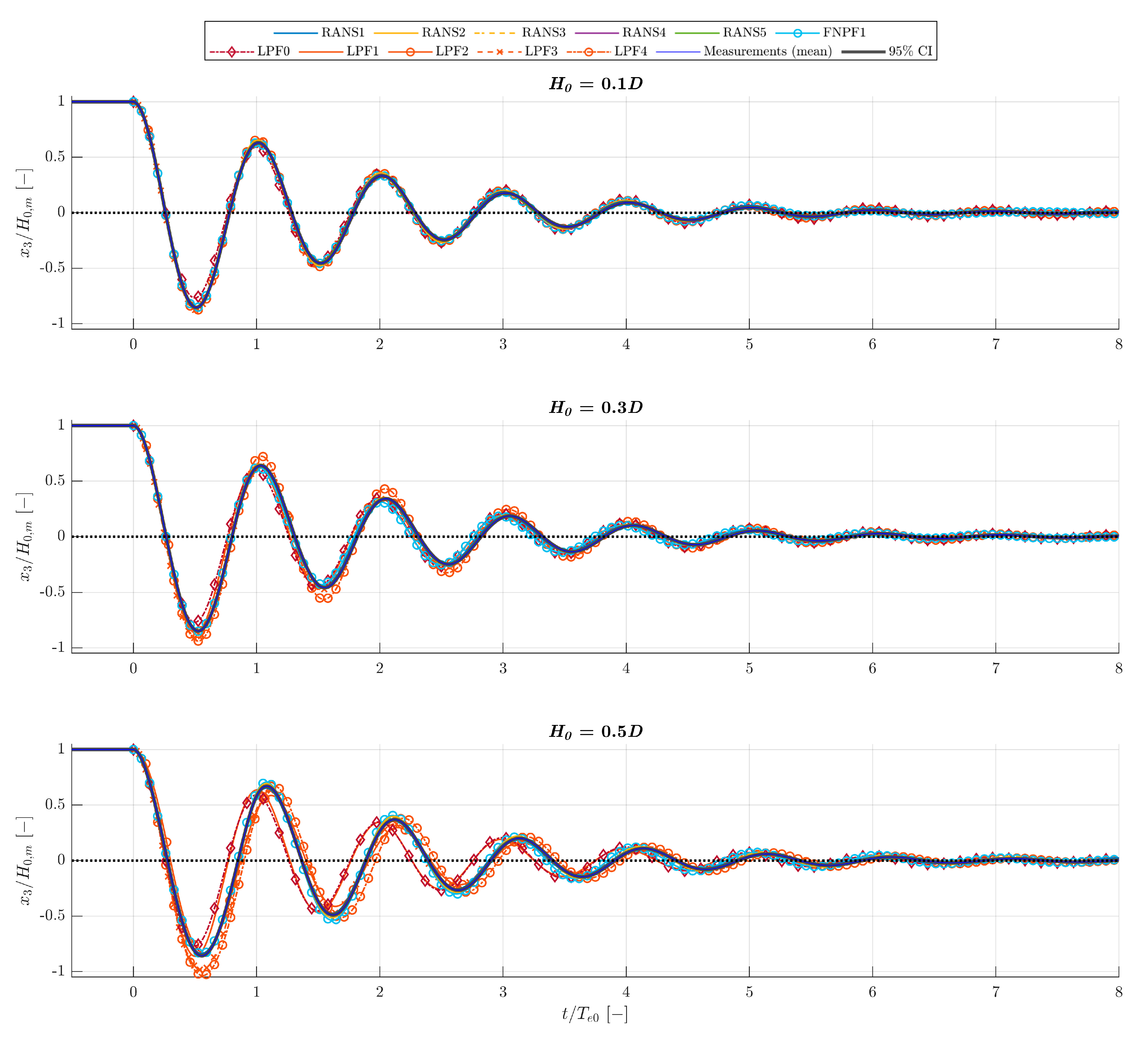
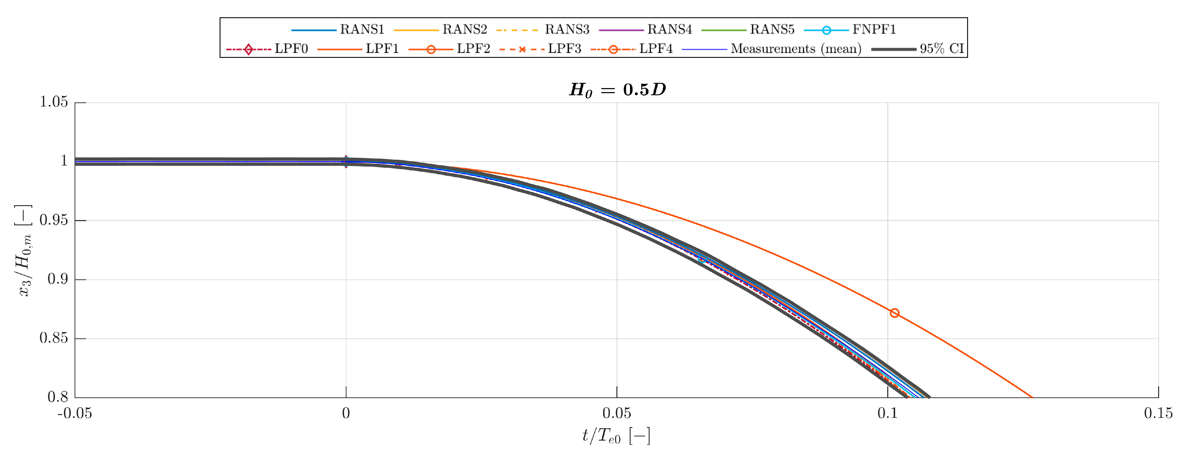
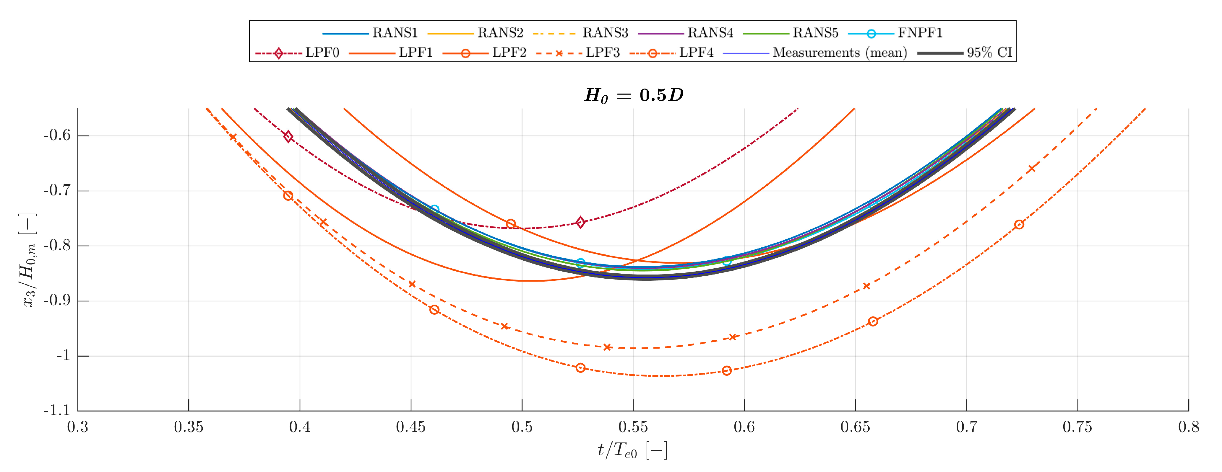
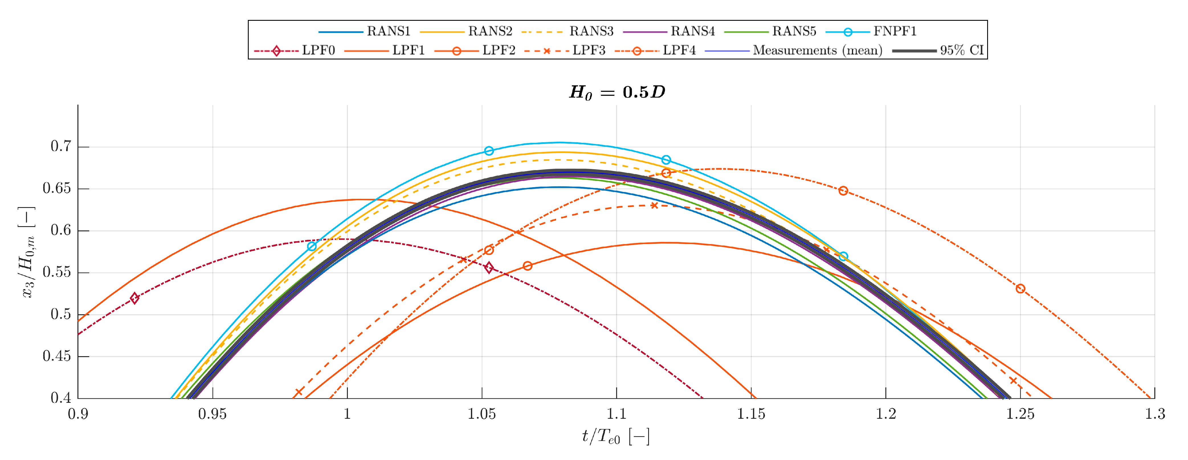
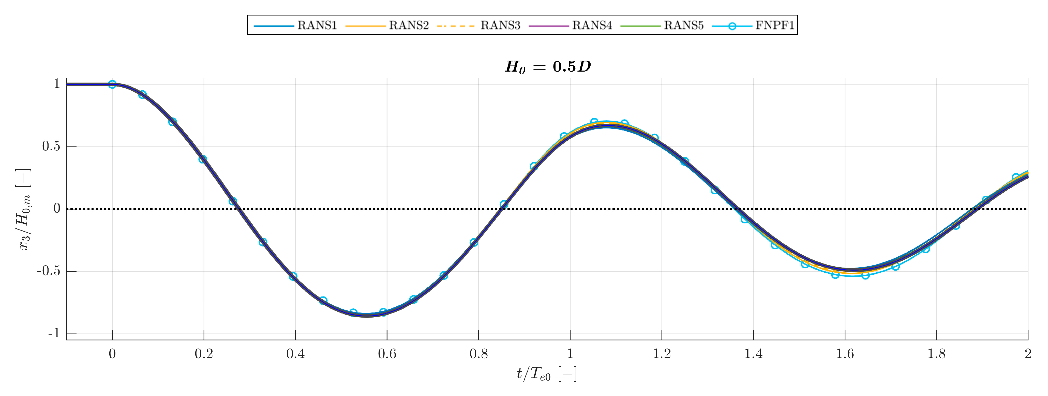
3.7. Comparison of Decay Measurements to Numerical Modelling Blind Tests
4. Discussion
Comparison to Numerical Modelling Blind Tests
5. Conclusions
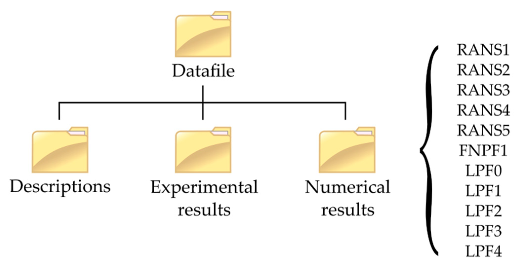
Supplementary Materials
Author Contributions
Funding
Acknowledgments
Conflicts of Interest
Appendix A


Appendix B

| Name | Institution and Authors | Framework | Description | Comp. Effort [CH] * |
|---|---|---|---|---|
| RANS1 | Aalborg University; C.E., J.A. | OpenFOAM-v1912 | 3D URANS model. Incompressible, isothermal. Volume of fluid method. Two vertical symmetry planes. Reflective side walls. Mesh morphing using SLERP method. Cell count of 6-9 M cells. No turbulence model. Second-order accurate in time and space. CFL criterion of 0.5 | ~3000–6500 |
| RANS2 | University of Plymouth; E.R., S.B. | OpenFOAM 5.0 | 3D URANS model. Incompressible, isothermal. Volume of fluid. Two vertical symmetry planes. Reflective side walls. Mesh morphing using SLERP method. Cell count of ~12 M cells. No turbulence model. CFL criterion of 0.5. | ~1000–4200 |
| RANS3 | University of Plymouth; E.R., S.B. | OpenFOAM 5.0 | Same as RANS2 except k-Omega SST turbulence model. Only conducted for H0 = 0.5D. | ~1800 |
| RANS4 | National Renewable Energy Lab.; Y.-H.Y., T.T.T. | STAR-CCM+ 13.06 | 3D URANS model. Incompressible, isothermal. Volume of fluid. Two vertical symmetry planes. Cell count of 6 M cells. Mesh morphing with one DOF. k-Omega SST turbulence model. second-order accurate in time and space. CFL criterion of 0.5. Max. time step of 0.1 ms. | ~1000–2600 |
| RANS5 | Budapest University of Technology and Economics; J.D., C.H. | OpenFOAM 7 | 2D URANS model. Incompressible, isothermal. Volume of fluid method. Axisymmetric wedge geometry. Cell count of approx. 20 K cells. No turbulence model. second-order accurate in time and space. CFL criterion of 0.25. Water depth changed to 1.8 m to allow mesh morphing. | ~0.5–2.5 |
| FNPF1 | Chalmers University of Technology; C.-E.J. | SHIPFLOW-Motions 6 | Fully nonlinear potential flow BEM. 1600 panels were used on the sphere and 4600 panels were used on the free surface. The time step was 0.005 s. | ~6 |
| LPF0 | Aalborg University; M.B.K., J.A. | WAMIT and MatLab | Analytical solution to one-DoF mass-spring-damper system with hydrodynamic coefficients from BEM (for ω = ωe0) | - ** |
| LPF1 | Floating Power Plant; M.B.K. | WAMIT and MatLab/Simulink | Model with linear hydrostatics and linear coefficients from BEM. Time-step: 1 ms, solver: ode4 (Runge-Kutta). | - ** |
| LPF2 | Floating Power Plant; M.B.K. | WAMIT and MatLab/Simulink | Model with nonlinear hydrostatics and linear coefficients from BEM. Time-step: 1 ms, solver: ode4 (Runge-Kutta). | - ** |
| LPF3 | Floating Power Plant; M.B.K. | WAMIT and MatLab/Simulink | Model with nonlinear hydrostatics, linear radiation function from linear BEM but position dependent infinity added mass. Time-step: 1 ms, solver: ode4 (Runge-Kutta). | - ** |
| LPF4 | Floating Power Plant; M.B.K. | WAMIT and MatLab/Simulink | Model with nonlinear hydrostatics and position dependent radiation functions (based on linear coefficients from BEM). Time-step: 1 ms, solver: ode4 (Runge-Kutta). | - ** |
Appendix C
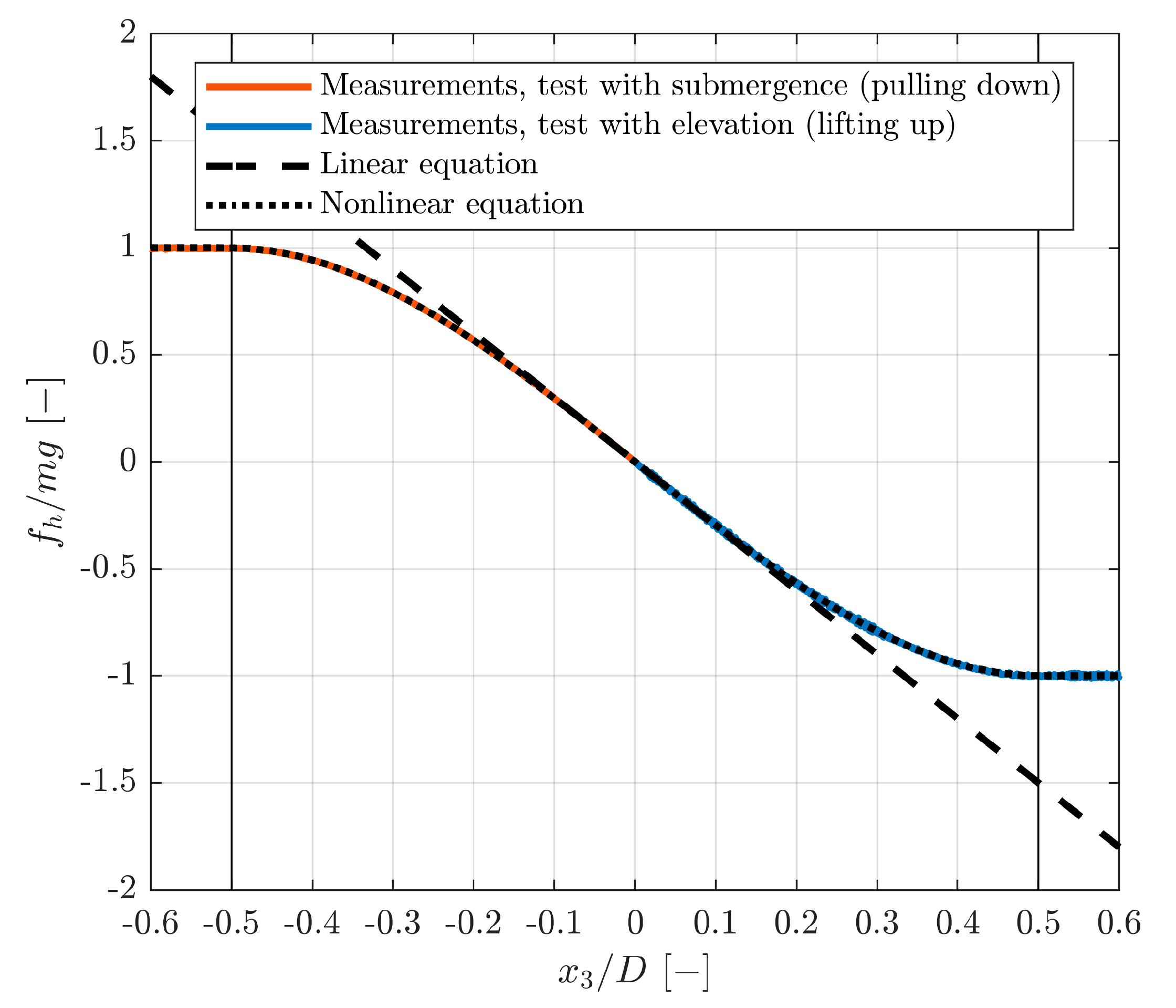
Appendix C.1. Linearization of Hydrostatics
Appendix C.2. The LPF0 Model
| Te0 | ωe0 | δ | A33(ωe0) | B33(ωe0) | C33 | C1 | C2 |
|---|---|---|---|---|---|---|---|
| [s] | [rad/s] | [rad/s] | [kg] | [Ns/m] | [N/m] | [m] | [m] |
| 0.76 | 8.30 | 0.695 | 2.97 | 13.95 | 692.89 | H0 | 0.0839H0 |
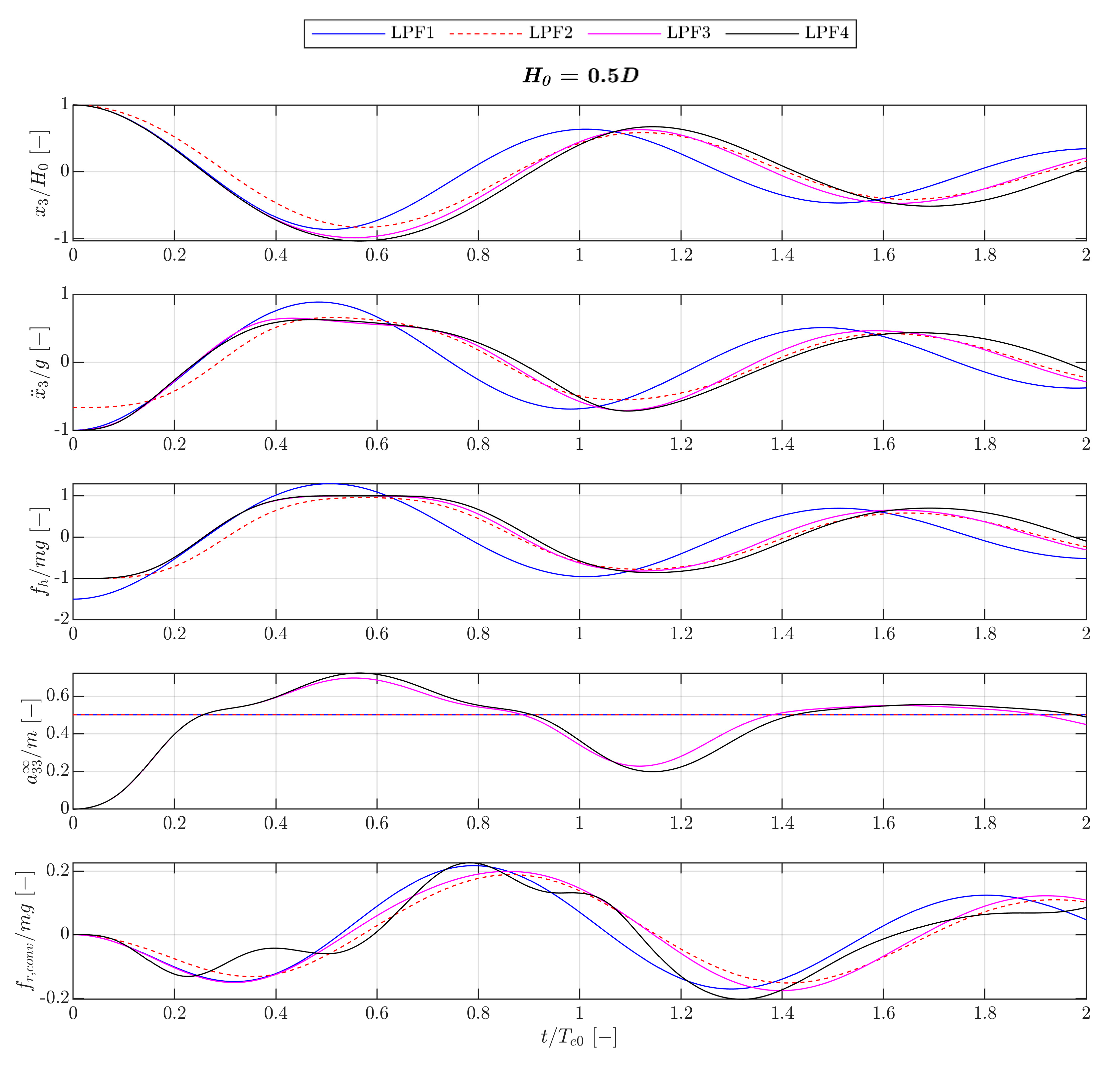
Appendix C.3. The LPF1–4 Models
| Model | Hydrostatics C3 | Radiation Convolution Function K33 | |
|---|---|---|---|
| LPF1 | Constant | Constant | Constant function |
| LPF2 | Draft-dependent | Constant | Constant function |
| LPF3 | Draft-dependent | Draft-dependent | Constant function |
| LPF4 | Draft-dependent | Draft-dependent | Draft-dependent functions |
Appendix C.4. Measured Hydrostatics

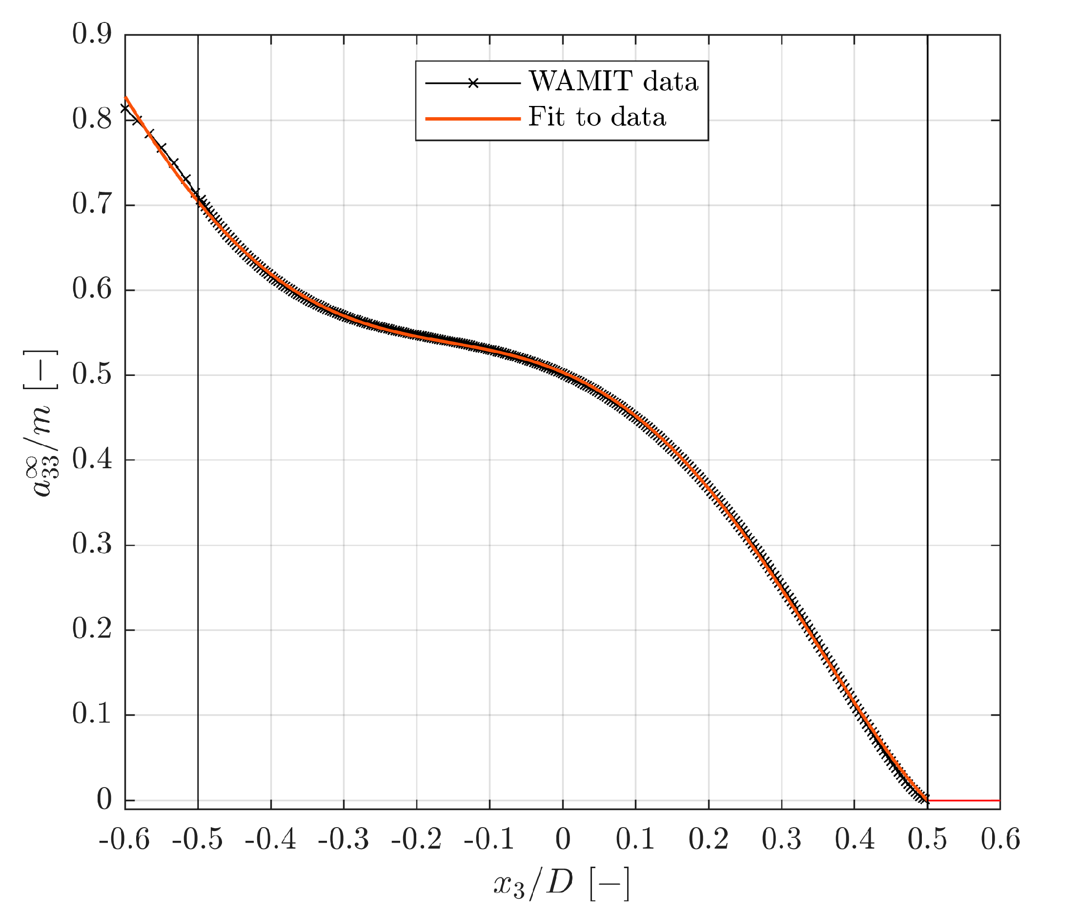
Appendix C.5. Added Mass at Infinite Frequency

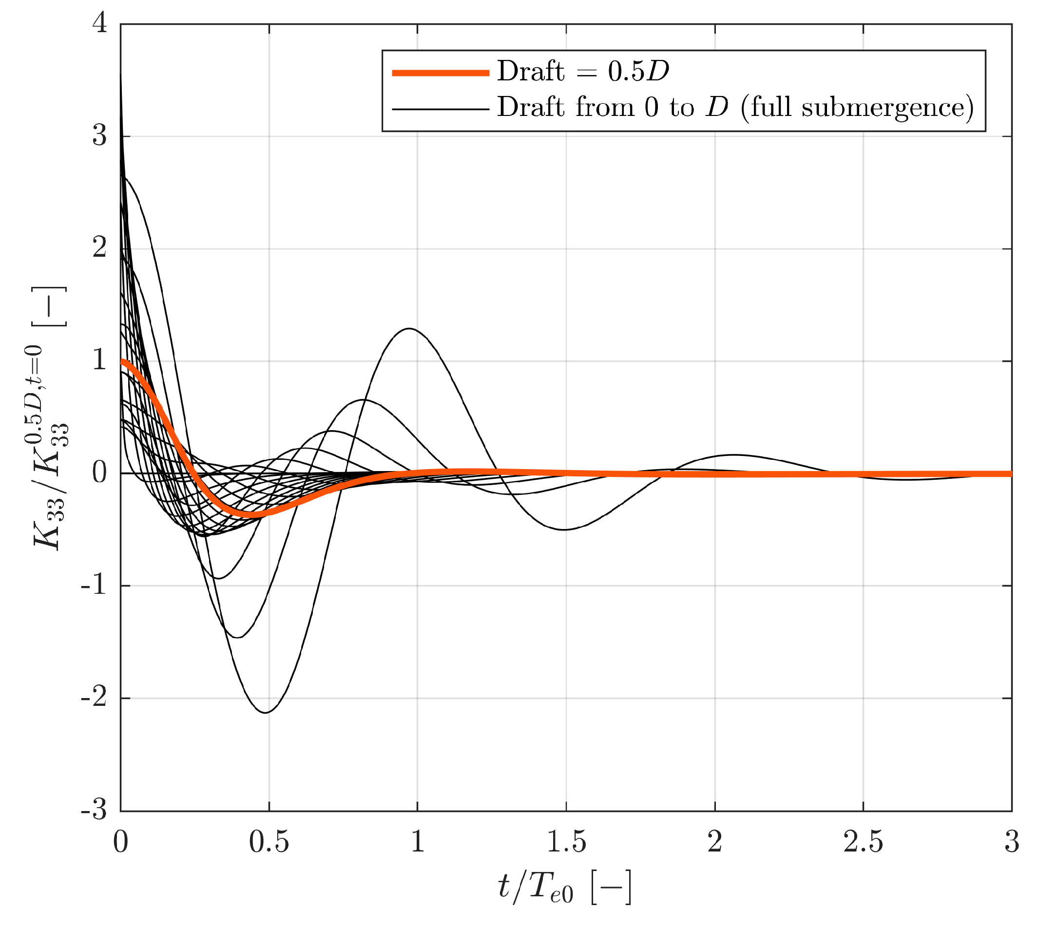
Appendix C.6. Radiation IRF

Appendix C.7. Comparison of the LPF1–4 Models

Appendix D


References
- Devolder, B.; Stratigaki, V.; Troch, P.; Rauwoens, P. CFD Simulations of Floating Point Absorber Wave Energy Converter Arrays Subjected to Regular Waves. Energies 2018, 11, 641. [Google Scholar] [CrossRef]
- Windt, C.; Davidson, J.; Ransley, E.J.; Greaves, D.; Jakobsen, M.; Kramer, M.; Ringwood, J.V. Validation of a CFD-based numerical wave tank model for the power production assessment of the Wavestar ocean energy converter. Renew. Energy 2019, 146, 2499–2516, ISSN 0960-1481. [Google Scholar] [CrossRef]
- Pecher, A.F.S.; Kofoed, J.P. (Eds.) Handbook of Ocean Wave Energy; Ocean Engineering & Oceanography; Springer: Berlin/Heidelberg, Germany, 2017; Volume 7. [Google Scholar] [CrossRef]
- Ransley, E.; Yan, S.; Brown, S.; Hann, M.; Graham, D.; Windt, C.; Schmitt, P.; Davidson, J.; Ringwood, J.; Wang, M.; et al. A blind comparative study of focused wave interactions with floating structures (CCP-WSI Blind Test Series 3). Int. J. Offshore Polar Eng. 2020, 30, 1–10. [Google Scholar] [CrossRef]
- IEA OES Wave Energy Converters Modelling Verification and Validation. Available online: https://www.ocean-energy-systems.org/oes-projects/wave-energy-converters-modelling-verification-and-validation/ (accessed on 22 July 2020).
- Wendt, F.; Nielsen, K.; Yu, Y.-H.; Bingham, H.; Eskilsson, C.; Kramer, M.; Babarit, A.; Bunnik, T.; Costello, R.; Crowley, S.; et al. Ocean Energy Systems Wave Energy Modelling Task: Modelling, Verification and Validation of Wave Energy Converters. J. Mar. Sci. Eng. 2019, 7, 379. [Google Scholar] [CrossRef]
- Nielsen, K.; Wendt, F.; Yu, Y.-H.; Ruehl, K.; Touzon, I.; Nam, B.W.; Kim, J.S.; Kim, K.-H.; Crowley, S.; Wanan, S.; et al. OES Task 10 WEC heaving sphere performance modelling verification. In Advances in Renewable Energies Offshore, Proceedings of the 3rd International Conference on Renewable Energies Offshore (RENEW 2018), Lisbon, Portugal, 8–10 October 2018, 1st ed.; Guedes Soares, C., Ed.; CRC Press: London, UK, 2018; pp. 265–273. [Google Scholar]
- Wendt, F.; Yu, Y.-H.; Nielsen, K.; Ruehl, K.; Bunnik, T.; Touzon, I.; Nam, B.W.; Kim, J.S.; Kim, K.-H.; Janson, C.E.; et al. International Energy Agency Ocean Energy Systems Task 10 Wave Energy Converter Modelling Verification and Validation. In Proceedings of the 12th EWTEC—European Wave and Tidal Energy Conference, Cork, Ireland, 27 August–1 September 2017; Volume 12. [Google Scholar]
- OES Task10 WEC Modelling, Verification & Validation. Available online: https://energiforskning.dk/node/9035 (accessed on 22 July 2020).
- Kramer, M. Highly Accurate Experimental Tests with a Floating Sphere—Kramer Sphere Cases. OES TASK 10 WEC Modelling Workshop 3 on 14 and 15 of November 2019, Amsterdam. Available online: https://www.wecanet.eu/oes-task-10-workshop (accessed on 4 January 2021).
- ASME. ASME PTC 19.1-2018: Test Uncertainty (Performance Test Code); ASME: New York, NY, USA, 2019. [Google Scholar]
- ISO/IEC. Guide 98-3 Uncertainty of Measurement—Part 3: Guide to the Expression of Uncertainty in Measurement (GUM:1995), 1st ed.; ISO/IEC: Geneve, Switzerland, 2008. [Google Scholar]
- Windt, D.; Davidson, J.; Ringwood, J. High-fidelity numerical modelling of ocean wave energy systems: A review of computational fluid dynamics-based numerical wave tanks. Renew. Sustain. Energy Rev. 2018, 93, 610–630. [Google Scholar] [CrossRef]
- Yang, Z. Assessment of unsteady-RANS approach against steady-RANS approach for predicting twin impinging jets in a cross-flow. Cogent Eng. 2014, 1, 1. [Google Scholar] [CrossRef]
- Weller, H.; Taber, G.; Jasak, H.; Fureby, C. A tensorial approach to computational continuum mechanics using object-oriented techniques. Comput. Phys. 1998, 12, 620–631. [Google Scholar] [CrossRef]
- STAR-CCM+, Siemens Digital Industries Software. Available online: https://www.plm.automation.siemens.com/global/en/products/simcenter/STAR-CCM.html (accessed on 31 August 2020).
- Deshpande, S.; Anumolu, L.; Trujillo, M.F. Evaluating the performance of the two-phase flow solver interFoam. Comput. Sci. Discov. 2012, 5, 014016. [Google Scholar] [CrossRef]
- Davidson, J.; Costello, R. Efficient Nonlinear Hydrodynamic Models for Wave Energy Converter Design—A Scoping Study. J. Mar. Sci. Eng. 2020, 8, 35. [Google Scholar] [CrossRef]
- Grilli, S. Fully Nonlinear Potential Flow Models Used for Long Wave Runup Prediction. 1996. Available online: https://personal.egr.uri.edu/grilli/long-97.pdf (accessed on 27 August 2020).
- SHIPFLOW Motions, FLOWTECH International AB. Available online: https://www.flowtech.se/products/shipflow-motions (accessed on 31 August 2020).
- Longuet-Higgins, M.S.; Cokelet, E.D. The deformation of steep surface waves—I. A numerical method of computation. Proc. R. Soc. Lond. 1976, 350, 1–26. [Google Scholar] [CrossRef]
- Janson, C.-E.; Shiri, A.; Jansson, J.; Moragues, M.; Castanon, D.; Saavedra, L.; Degirmenci, C.; Leoni, M. Nonlinear computations of heave motions for a generic Wave Energy Converter. In Proceedings of the NAV 2018, 19th International Conference on Ships and Maritime Research, Trieste, Italy, 20–22 June 2018; Marinò, A., Bucci, V., Eds.; IOS Press BV: Amsterdam, The Netherlands, 2018. [Google Scholar]
- Ferrandis, J.D.Á.; Bonfiglio, L.; Rodríguez, R.Z.; Chryssostomidis, C.; Faltinsen, O.M.; Triantafyllou, M. Influence of Viscosity and Nonlinearities in Predicting Motions of a Wind Energy Offshore Platform in Regular Waves. J. Offshore Mech. Arct. Eng. 2020, 142, 062003. [Google Scholar] [CrossRef]
- Wehausen, J.V.; Laitone, E.V. Surface Waves in Fluid Dynamics III. In Handbuch der Physik 9; Flugge, S., Truesdell, C., Eds.; Springer: Berlin, Germany, 1960; pp. 446–778. [Google Scholar]
- Newman, J. Marine Hydrodynamics; MIT Press: Cambridge, MA, USA, 1977; ISBN 9780262140263. [Google Scholar]
- Faltinsen, O. Sea Loads on Ships and Offshore Structures; Cambridge University Press: Cambridge, UK, 1990; ISBN 0521458706. [Google Scholar]
- Cummins, W.E. The Impulse Response Function and Ship Motions. Schiffstechnik 1962, 9, 101–109. [Google Scholar]
- Falnes, J. Ocean. Waves and Oscillating Systems—Linear Interactions Including Wave-Energy Extraction; Cambridge University Press: Cambridge, UK, 2002; ISBN 9780511754630. [Google Scholar]
- Lee, C.H.; Newman, J.N. WAMIT User Manual Version 7.3; WAMIT, Inc.: Chestnut Hill, MA, USA, 2019. [Google Scholar]
- Ayyub, B.M.; McCuen, R.H. Probability, Statistics, and Reliability for Engineers and Scientists, 2nd ed.; Chapman & Hall/CRC: Boca Raton, FL, USA, 2003; ISBN 1-58488-286-7. [Google Scholar]
- Brorsen, M.; Larsen, T. Lærebog i Hydraulik (Danish), 2nd ed.; Aalborg Universitetsforlag: Aalborg, Denmark, 2009; ISBN 978-87-7307-978-2. [Google Scholar]
- Carter, S.; Gutierrez, G.; Batavia, M. The Reliability of Qualisys’ Oqus System. In Proceedings of the APTA NEXT 2015 Conference and Exposition, National Harbor, MD, USA, 3–6 June 2015. [Google Scholar]


| Parameter | D | m | CoG | g | H0 | ρw | d |
|---|---|---|---|---|---|---|---|
| Unit | mm | kg | mm | m/s2 | mm | kg/m3 | mm |
| Value | 300 | 7.056 | (0, 0, −34.8) | 9.82 | {30 90 150} | 998.2 | 900 |
| Parameter | M | CoG | Ixx | Iyy | Izz | Ixz | Ixy, Iyz |
|---|---|---|---|---|---|---|---|
| Unit | g | mm | gmm2 | gmm2 | gmm2 | gmm2 | gmm2 |
| Value | 7056 | (0, 0, −34.8) | 98251·103 | 98254·103 | 73052·103 | 0·103 | 10·103 |
| Systematic Error Source k | ISO Types | |
|---|---|---|
| Calibration of motion capture system (Oqus7+) | 0.01 | A |
| Vibrations of bridge (reference frame) | 0.01 | B |
| Vibration of support rods for reflective markers (for ascending H0) | 0.02, 0.06, 0.10 | B |
| Influence on heave measurements from roll and pitch | Time-dependent, <0.02 | A |
| Parameter | Value | Standard Uncertainty | Unit | ISO Type | |
|---|---|---|---|---|---|
| Test case values | Diameter of sphere | 300 | 0.1 | mm | B |
| Mass of sphere | 7056 | 1 | g | B | |
| Centre of gravity | (0.0, 0.0, −34.8) | (0.1, 0.1, 0.1) | mm | B | |
| Acceleration due to gravity | 9.82 | 0.003 | m/s2 | B | |
| Drop heights (mean); H0 = {0.1D,0.3D,0.5D} | {29.16, 89.18, 150.06} | {0.8, 0.5, 0.3} | mm | A | |
| Density of water [31] | 998.2 | 0.4 | kg/m3 | B | |
| Water depth | 900 | 1 | mm | B | |
| Initial velocity in heave | 0.0000 | 0.0004 | m/s | A | |
| Initial acceleration in heave | −0.0002 | 0.0097 | m/s2 | A | |
| Additional values (Recommended for high-fidelity models) | Temperature of air and water | 20 | 2 | °C | B |
| Kinematic viscosity of water [31] | 1.0·10−6 | 0.1·10−6 | m2/s | B | |
| Density of air [31] | 1.20 | 0.012 | kg/m3 | B | |
| Kinematic viscosity of air [31] | 15.1·10−6 | 0.2·10−6 | m2/s | B | |
| Surface tension water-air [31] | 0.07 | 0.004 | N/m | B | |
| Moments of inertia of the sphere model; I = {Ixx,Iyy,Izz,Ixy,Ixz,Iyz} | {98251, 98254, 73052, 0, 10, 0}·103 | {37, 37, 1, 0, −77, 96}·103 | gmm2 | B | |
| Initial surface elevation | 0.0 | 0.01 | mm | A |
Publisher’s Note: MDPI stays neutral with regard to jurisdictional claims in published maps and institutional affiliations. |
© 2021 by the authors. Licensee MDPI, Basel, Switzerland. This article is an open access article distributed under the terms and conditions of the Creative Commons Attribution (CC BY) license (http://creativecommons.org/licenses/by/4.0/).
Share and Cite
Kramer, M.B.; Andersen, J.; Thomas, S.; Bendixen, F.B.; Bingham, H.; Read, R.; Holk, N.; Ransley, E.; Brown, S.; Yu, Y.-H.; et al. Highly Accurate Experimental Heave Decay Tests with a Floating Sphere: A Public Benchmark Dataset for Model Validation of Fluid–Structure Interaction. Energies 2021, 14, 269. https://doi.org/10.3390/en14020269
Kramer MB, Andersen J, Thomas S, Bendixen FB, Bingham H, Read R, Holk N, Ransley E, Brown S, Yu Y-H, et al. Highly Accurate Experimental Heave Decay Tests with a Floating Sphere: A Public Benchmark Dataset for Model Validation of Fluid–Structure Interaction. Energies. 2021; 14(2):269. https://doi.org/10.3390/en14020269
Chicago/Turabian StyleKramer, Morten Bech, Jacob Andersen, Sarah Thomas, Flemming Buus Bendixen, Harry Bingham, Robert Read, Nikolaj Holk, Edward Ransley, Scott Brown, Yi-Hsiang Yu, and et al. 2021. "Highly Accurate Experimental Heave Decay Tests with a Floating Sphere: A Public Benchmark Dataset for Model Validation of Fluid–Structure Interaction" Energies 14, no. 2: 269. https://doi.org/10.3390/en14020269
APA StyleKramer, M. B., Andersen, J., Thomas, S., Bendixen, F. B., Bingham, H., Read, R., Holk, N., Ransley, E., Brown, S., Yu, Y.-H., Tran, T. T., Davidson, J., Horvath, C., Janson, C.-E., Nielsen, K., & Eskilsson, C. (2021). Highly Accurate Experimental Heave Decay Tests with a Floating Sphere: A Public Benchmark Dataset for Model Validation of Fluid–Structure Interaction. Energies, 14(2), 269. https://doi.org/10.3390/en14020269