Design of a Neural Super-Twisting Controller to Emulate a Flywheel Energy Storage System

Abstract

In this work, a neural super-twisting algorithm is applied to the design of a controller for a flywheel energy storage system (FESS) emulator. Emulation of the FESS is achieved through driving a Permanent Magnet Synchronous Machine (PMSM) coupled to a shaft to shaft DC-motor. The emulation of the FESS is carried out by controlling the velocity of the PMSM in the energy storage stag and then by controlling the DC-motor velocity in the energy feedback stage, where the plant’s states of both electrical machines are identified via a neural network. For the neural identification, a Recurrent Wavelet First-Order Neural Network (RWFONN) is proposed. For the design of the velocity controller, a super-twisting algorithm is applied by using a sliding surface as the argument; the latter is designed based on the states of the RWFONN, in combination with the block control linearization technique to the control of the angular velocity from both machines in their respective operation stage. The RWFONN is trained online using the filtered error algorithm. Closed-loop stability analysis is included when assuming boundedness of the synaptic weights. The results obtained from Matlab/Simulink validate the performance of the proposal in the control of an FESS.

1. Introduction

For many years, flywheels made of stone or other primitive materials have been used for the operation of different mechanisms. Currently, there are mechanisms built from metal flywheels, powered by electric motors, which can work in both motor and generator mode and whose main function is to store energy in the flywheel; because of this property, these mechanisms are known as Flywheel Energy Storage Systems (FESSs) [1]. Induction motors and synchronous motors are some types of electrical machines used in the application of FESSs. For the proper functioning of the electrical grid, it is essential to have a balance between consumption and supply of electrical energy. Due to its rapid response of operation, an FESS has the ability to reduce some of the problems caused by power variations. The control and comparison between different electrical machines used in FESSs are shown in [2]. The FESSs have been studied by different authors showing the performance from different control strategies. Furthermore, in several published works, a complete FESS has been emulated through the use of electric motors where the main operation of the flywheel is the storage of mechanical energy in a rotating flywheel, which can then be converted to electrical energy using an electrical machine with power inverters [3]. An FESS has several advantages in contrast with other energy storage systems, including long useful life, and an FESS has multiple applications such as in wind generators, electric vehicles, etc. [4]. In [5], a vector control strategy was presented to emulate a FESS using a DC permanent magnet machine, where the machine was coupled to a PMSM to control the angular velocity of the flywheel in the charging and discharging stages. In [6], an integral sliding mode controller with a super-twisting algorithm was presented. In that work, the rotor side converter in the doubly-fed induction generator is used for controlling a wind generator, where the sliding surfaces are generated such that these are compatible with the errors in the stator active and reactive powers. In [7], emulation of an FESS using reconfigurable hardware test-bed of power converters was presented, where the emulation was carried out to the acceleration, deceleration and standby modes. The flywheel’s model is described in the $dq$ domain with relations among voltage, current and rotating speed. In [8], an adaptive control for high-speed FESSs was proposed where the controller has the task of controlling the DC-link voltage for the FESS and controlling the active power exchange between the FESS and the grid, whose advantage of inertia emulation is that the inertia and damping can be altered in real-time. In [9], under the assumption that all the states are measurable, a sliding mode control system for a 4-quadrant DC–DC converter was designed. Furthermore, a low voltage prototype for a flywheel application was constructed.

Recently, a control scheme applied to an FESS for the improvement of the dynamic performance of the utility grid, based on a PMSM incorporated into a multi-machine system, was presented in [10]. In that work, the speed and voltages generated were monitored by the FESS in order to generate the real and reactive power. Such control strategy was designed against three-phase faults.

On the one hand, considering that the fundamental parts of an energy storage system are the electric motors, the PMSM is a kind of synchronous motor that features low inertia, low noise, high power density and high efficiency, simple structure, and easy control. PMSMs have been used for the control of robotic movements, electric and aerospace propulsions, etc. [11]. The nonlinear mathematical model of a PMSM is strongly coupled. In addition, its parameters are not fixed but are kept within an operating range depending on the work environment. Angular velocity and torque can fluctuate in some parameter regions [12]. Recently, a feedback technique of dynamic surface control for a chaotic PMSM, based on nonlinear mappings using neural networks (NNs) to approximate the system dynamics as well as to estimate the unknown parameters, has been proposed in [13]. In [14], NNs were implemented in a PMSM for the detection of damage or failure in motor bearings by analyzing mechanical vibrations, comparing different types of NNs and the effectiveness of failure detection.

On the other hand, DC machines are generators that convert mechanical energy into DC electrical energy and motors that convert DC electrical energy into mechanical energy. Most DC machines are similar to alternating current machines in that they have AC voltages and currents inside them. DC machines have a DC output only because there is a mechanism that converts internal AC voltages into DC voltages at their terminals; since this mechanism is called a commutator, DC machinery is also known as a commutator or commutator machinery [15].

Implementation of the sliding-mode control to DC motors has been studied by different authors. In [16], an adaptive neural controller in discrete-time was proposed, where a NN was used to identify the plant model, using the Kalman extended filter training algorithm, when applying the block control in sliding mode for angular velocity control. A speed control scheme for a DC motor, based on state observers of sliding modes, was presented in [17]. In that work, the state observers estimate the angular velocity and the load torque; thus, in this way, it was possible to apply the controller, designed from the application of the exact linearization technique in combination with the super- twisting control.

The application of super-twisting control has been recently studied in [18], introducing the control to roll suppression of marine vessels subjected to harmonic wave excitations, where some of the main control objectives were to reduce the phenomenon of vibration over dynamic behaviors such as chaos, due to parametric variation.

The main contribution of this work is the proposal of a methodology to emulate a flywheel energy storage system by driving a motor-generator group formed by two machines, namely, a PMSM coupled with a DC-motor. The state variables of the system are identified via recurrent wavelet NNs of first-order trained online by the filtered error algorithm. By using these NNs, it is possible to involve unmodeled dynamics and parameter variations, avoiding uncertainty in the machine parameters. The PMSM velocity controller is designed to emulate the stored kinetic energy of the flywheel, while the DC-motor velocity controller is used to emulate the energy that is discharged towards the utility grid. Both controllers are synthesized based on the proposed NN model transformed into the block controllable form to define a sliding surface that is steered to the origin in finite time by the action of the super-twisting control algorithm.

This paper is organized as follows. In Section 2, the mathematical background is presented, which is related to the kinetic energy storage, identification of the nonlinear system via recurrent wavelet first order neural network (RWFONN) using the filtered error training algorithm, and the super-twisting control algorithm; Section 3 presents the proposed methodology, where the procedures of charge/discharge are explained in detail; in Section 4, the simulation results are shown, from which the proposed methodology is validated; some important discussions are presented in Section 5; conclusion and some remarks about the application of the Neural Super-Twisting Control (NSTC) are drawn in Section 6. Furthermore, in Appendix A and Appendix B, the boundedness of the identification error and the complete closed-loop stability analysis are shown, respectively.

2. Mathematical Background

This section describes the energy storage in an FESS, the nonlinear mathematical representation of a permanent magnet synchronous motor and a DC-motor, the mathematical model of the dynamic behavior for an RWFONN and summarizes the filtered error algorithm, the block control linearization technique, and the super-twisting control algorithm.

2.1. FESS

The main function of FESSs is to store rotational kinetic energy, which can then be converted into electrical energy by means of an electric machine. In order to generate rotational kinetic energy, the flywheel must be driven by an electric machine that meets the requirement of operating in both motor and generator mode, allowing to convert rotational kinetic energy into electric energy and vice versa [4]. The main components from an FESS are the steering wheel, a vacuum containment to avoid loss by air friction, magnetic or metallic bearings, an electric machine capable of operating in both operation modes, i.e., motor and generator mode, and a three-phase converter to connect the FESS with the utility-grid [1]. The kinetic energy stored in the flywheel can be approximated by the following equation [19]

$$\begin{array}{c}\hfill E_k=\frac{1}{2}{J}_m{\omega }_m^2,\end{array}$$

(1)

where $E_k$ is the stored kinetic energy in J, $J_m$ is the inertial moment in N·m·s${}^2$, and ${\omega }_m$ is the rated angular velocity in rad/s. In order to emulate the FESS deceleration, it is considered the next equation

$$\begin{array}{c}\hfill \frac{d}{dt}{\omega }_m=\frac{-B_m{\omega }_m}{J_m},\end{array}$$

(2)

which defines the mechanical behavior of the flywheel when the energy is delivered to the utility grid [20], with $B_m$ the frictional coefficient in N·m·s.

2.2. Nonlinear Systems

A class of nonlinear multi-input/multi-output system given in the general form

$$\dot{\chi }=\mathbf{f}(\chi ,t)+\mathbf{B}(\chi ,t)\mathbf{u}+\mathbf{g}(\chi ,t)$$

(3)

where $\chi \in \mathbf{X}\subset {\mathbb{R}}^n$ is the state vector of the system, $\mathbf{f}(\chi ,t)$ is the nonlinear system function vector; $\mathbf{u}\in \mathbf{U}\subset {\mathbb{R}}^m$ is the control input vector, $\mathbf{B}(\chi ,t)$ is a non-singular matrix that characterizes the system, and $\mathbf{g}(\chi ,t)$ is a smooth function vector that represents external disturbances and parametric variations. It must be noticed that in the present work, both PMSM and DC-motor mathematical models match with that given in the general form (3). It is important to mention that due to the purpose of this work, these mathematical models are not shown here.

2.3. RWFONN

First-order NNs are used for system identification as well as to design neural controllers for some electrical, mechanical or electromechanical systems. A novel neural identification scheme, namely a Recurrent Morlet Wavelet Neural Network (RMWNN) also known as RWFONN, based on a recurrent high-order neural network (RHONN) structure was proposed in [21]. In the NN propose in this work, the classical sigmoid activation function has been replaced by a Morlet wavelet function. The general structure from an RWFONN is given by [22]

$${\dot{x}}_j^i=-a_j^i{x}_j^i+{\left(w_{jk}^i\right)}^{\top }{\psi }_{jk}^i$$

(4)

where $x_j^i$ is the state of the i-th neuron, $a_j^i>0$ for $i=1,2,\dots ,n$ is part of the underlying network architecture and it is fixed during the training process, $w_{jk}^i$ is the k-th adjustable synaptic weight connecting the j-th state to the i-th neuron, and ${\psi }_{jk}^i$ is a Morlet wavelet activation function. The dynamic behavior of the whole neural network can be described by expressing Equation (4) in the vector notation

$$\begin{array}{cc}\hfill \dot{\mathbf{x}}=& \mathbf{A}\mathbf{x}+{\mathbf{w}}^{\top }\psi ,\hfill \end{array}$$

(5)

where $\mathbf{x}={\left[x_j^1{x}_j^2\dots x_j^n\right]}^{\top }\in {\mathbb{R}}^n$ is the state vector of the NN, $\mathbf{w}={\left[w_j^1{w}_j^2\dots w_j^n\right]}^{\top }$$\in {\mathbb{R}}^{L\times n}$ is the synaptic weights vector, with L representing the total number of weights used to identify the plant behavior, $\mathbf{A}=\mathrm{diag}\left[-a_j^1-a_j^2\dots -a_j^n\right]\in {\mathbb{R}}^{n\times n}$ is the parameter (Hurwitz) matrix, and $\psi$ is the regressor vector. In this work, $\psi \left(\chi \right)=e^{(-{\chi }^2/\beta )}\cos \left(\lambda \chi \right)$ is the Morlet wavelet function used here as the activation function where $\chi$ is the state from the plant (Equation (3)) and the parameters $\beta$, $\lambda$ are the expansion and dilation terms [22], respectively. Thus, the nonlinear system (3) is identified online by using an RWFONN (Equation (5)), where the synaptic weights vector $\mathbf{w}$ is adjusted via a filtered error algorithm.

2.4. Filtered Error Training Algorithm

For the application of the filtered error algorithm, this study begins under the assumption of an unknown system (3), which can be modeled (identified) by using an RWFONN structure (5). The synaptic weights are adjusted according to the following update law [23,24]

$$\begin{array}{c}\hfill {\dot{w}}_{jk}^i=-{\Gamma }_{jk}^i{\psi }_{jk}^i{\xi }_{jk}^i,\end{array}$$

(6)

where $\Gamma \in {\mathbb{R}}^{L\times L}$ is a definite positive gain matrix, $\psi$ is the Morlet wavelet activation function, and $\xi$ is the identification error, i.e., the difference between the states from the RWFONN (Equation (5)) and those from the plant (3), namely, ${\xi }_j^i=x_j^i-{\chi }_j^i$. The update law (Equation (6)) corresponds to the filtered error training algorithm [23]. Since the RWFONN is given in a generalized way from the structure for a RHONN, the following theorem establishes that identification and parametric errors for the RWFONN are bounded.

Theorem 1.

Consider the RWFONN model whose weights are adjustable according to Equation (6) for each $i=1,2,\dots ,n$;

1

${\xi }_j^i$, ${\mathbf{w}}_j^i$∈${\mathcal{L}}_{\infty }$ ($i.e.,{\xi }_j^i$ and $w_j^i$ are uniformly bounded);

2

${lim}_{t\to \infty }{\xi }_i\left(t\right)=0$.

Proof 

See [24,25]. □

Appendix A presents the boundedness of the identification error ${\xi }_j^i$ given by the synaptic weights $w_j^i$.

2.5. Nonlinear Block Controllable Form

One of the main characteristics of the block control linearization technique is to transform a nonlinear system into an equivalent form expressed by first-order subsystems consisting of r blocks, which can be solved independently one from each other. Such equivalent form is commonly known as the block controlled form whose representation is described by [26]

$$\begin{array}{cc}\hfill {\dot{\mathbf{x}}}_1=& {\mathbf{f}}_1({\mathbf{x}}_1,t)+{\mathbf{B}}_1({\mathbf{x}}_1,t)x_2+{\mathbf{g}}_1({\mathbf{x}}_1,t),\hfill \\ \hfill {\dot{\mathbf{x}}}_{\widehat{i}}=& {\mathbf{f}}_{\widehat{i}}({\overline{\mathbf{x}}}_{\widehat{i}},t)+{\mathbf{B}}_{\widehat{i}}({\overline{\mathbf{x}}}_{\widehat{i}},t){\mathbf{x}}_{\widehat{i}+1}+{\mathbf{g}}_{\widehat{i}}({\overline{\mathbf{x}}}_{\widehat{i}},t),\widehat{i}=2,\dots ,r-1,\hfill \\ \hfill {\dot{\mathbf{x}}}_r=& {\mathbf{f}}_r({\overline{\mathbf{x}}}_r,t)+{\mathbf{B}}_r({\overline{\mathbf{x}}}_r,t)\mathbf{u}+{\mathbf{g}}_r({\overline{\mathbf{x}}}_r,t),\hfill \end{array}$$

(7)

where $\mathbf{f}(\mathbf{x},t)$ is a smooth and bounded mapping, $\mathbf{x}={\left[x_1{x}_2\dots x_r\right]}^{\top }$ is the state vector decomposed, ${\overline{\mathbf{x}}}_{\widehat{i}}={\left[x_1\dots x_{\widehat{i}}\right]}^{\top }$, for $\widehat{i}=2,\dots ,r$, ${\mathbf{x}}_{\widehat{i}}$ is a $n_{\widehat{i}}\times 1$ vector, and the subscripts $(n_1,n_2,\dots ,n_r)$ define the structure of the system. The matrix ${\mathbf{B}}_{\widehat{i}}$, since the fictitious ${\mathbf{x}}_{\widehat{i}+1}$ for each $\widehat{i}$-th block has full rank, rank$\left({\mathbf{B}}_{\widehat{i}}\right)=n_{\widehat{i}}$, $\forall x\in X\subset {\mathbb{R}}^n$ and $t\in [0,\infty ]$, $\widehat{i}=1,\dots ,r$. Therefore, in this work, the block control technique is applied to the NN structure (5) to define a sliding surface, which is the argument of the super-twisting controller.

2.6. Super-Twisting Control Algorithm

The first-order sliding mode has long been used as a robust control technique to cancel nonlinear terms and uncertainties due to external disturbances in a system, but its main disadvantage is the presence of the chattering effect, which induces vibrations in the controlled system. In order to reduce the chattering effect, high-order sliding modes have been used. A particular case is the super-twisting algorithm (STA), which has been playing a very important role in sliding mode controllers. The super-twisting control (STC) algorithm of second-order can be applied to systems where the control appears in the first derivative of the sliding surface. The application of the STC allows to cancel perturbations and nonlinearities, forcing the sliding surface toward zero in finite time. Furthermore, the states that define the sliding surface are directed to zero with asymptotic motion. The dynamics of the sliding surface are known as sliding mode movement, and it is characterized by being a reduced-order system [27,28].

The sliding surface for the NSTC is defined from the nonlinear system once the latter resembles the block controllable form (7) for the variable on which the control input of the system appears. Therefore, the sliding surface is [29]

$$\begin{array}{cc}\hfill \mathbf{s}=& {\mathbf{x}}_r,\hfill \end{array}$$

(8)

where the dynamics of the sliding surface (Equation (8)), involving the STC algorithm and the system (7), take the form

$$\begin{array}{cc}\hfill \dot{\mathbf{s}}=& {\mathbf{f}}_r({\overline{\mathbf{x}}}_r,t)-{\mathbf{B}}_r({\overline{\mathbf{x}}}_r,t)({\lambda }_s{\left|\mathbf{s}\right|}^{\frac{1}{2}}\mathrm{sign}\left(\mathbf{s}\right)+{\mathbf{u}}_s)+{\mathbf{g}}_r({\overline{\mathbf{x}}}_r,t),\hfill \\ \hfill {\dot{\mathbf{u}}}_s=& {\alpha }_s\mathrm{sign}\left(\mathbf{s}\right),\hfill \end{array}$$

(9)

with ${\lambda }_s=\left[\begin{array}{cc}{\lambda }_{s11}& 0\\ 0& {\lambda }_{s22}\end{array}\right]$ and ${\alpha }_s=\left[\begin{array}{cc}{\alpha }_{s11}& 0\\ 0& {\alpha }_{s22}\end{array}\right]$ diagonal matrices. Then, the super-twisting control law provides finite-time convergence to zero, simultaneously $\mathbf{s}$ and $\dot{\mathbf{s}}$, where the term ${\lambda }_s{\left|\mathbf{s}\right|}^{\frac{1}{2}}\mathrm{sign}\left(\mathbf{s}\right)$ commutes its gain at high frequency for giving robustness to annul the nonlinearities ${\mathbf{f}}_r({\overline{\mathbf{x}}}_r,t)$, and to cancel the external disturbances ${\mathbf{g}}_r({\overline{\mathbf{x}}}_r,t)$, while the term ${\mathbf{u}}_s$ reduces the chattering effect and the steady state error [28].

In order to ensure the stability of the system with the super-twisting control law (Equation (9)), the control matrix gains $\lambda$ and $\alpha$ are holding to the following restrictions:

$$k_i>2{\delta }_i,k_i>\frac{1}{2}\frac{k_i^2({\delta }_i-k_i)}{k_i-2{\delta }_i}$$

(10)

where the disturbance norm is defined as $|{\mathbf{f}}_r({\overline{\mathbf{x}}}_r,t)+{\mathbf{g}}_r({\overline{\mathbf{x}}}_r{,t\left)\right|=\delta \left|s\right|}^{1/2}$, for $\delta >0$. The inequalities in Equation (10) are defined in the stability analysis presented in Appendix B.

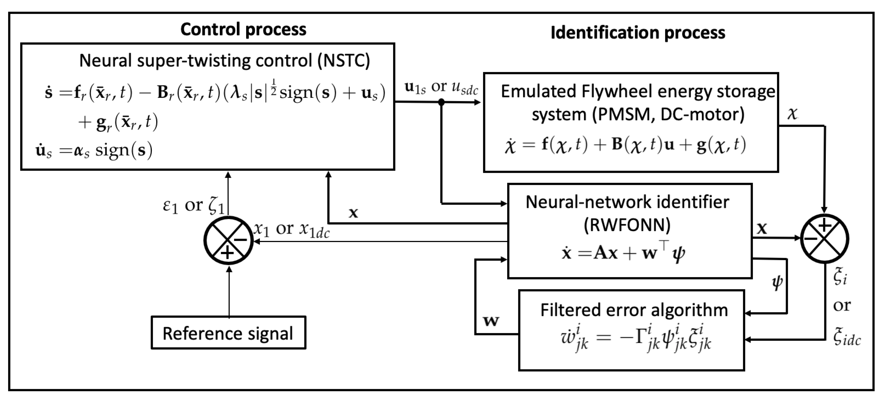
3. Proposed Methodology

This section describes the procedure for emulating the FESS through a group motor-generator formed by two electrical machines mechanically coupled. The angular velocity of the PMSM, when it is working in motor mode, is controlled in order to emulate the storing of energy, whereas the velocity for the DC-machine is controlled emulating the discharge of the flywheel where the PMSM is now working in generator mode. The FESS’s emulator scheme is shown in Figure 1. The procedure followed to the emulation of the FESS is explained next:

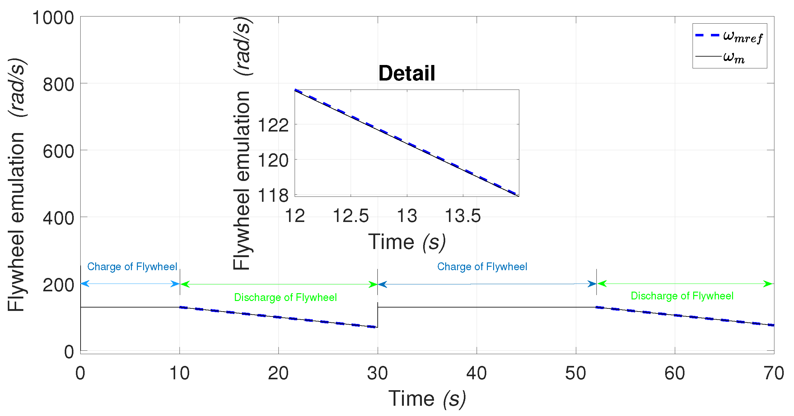
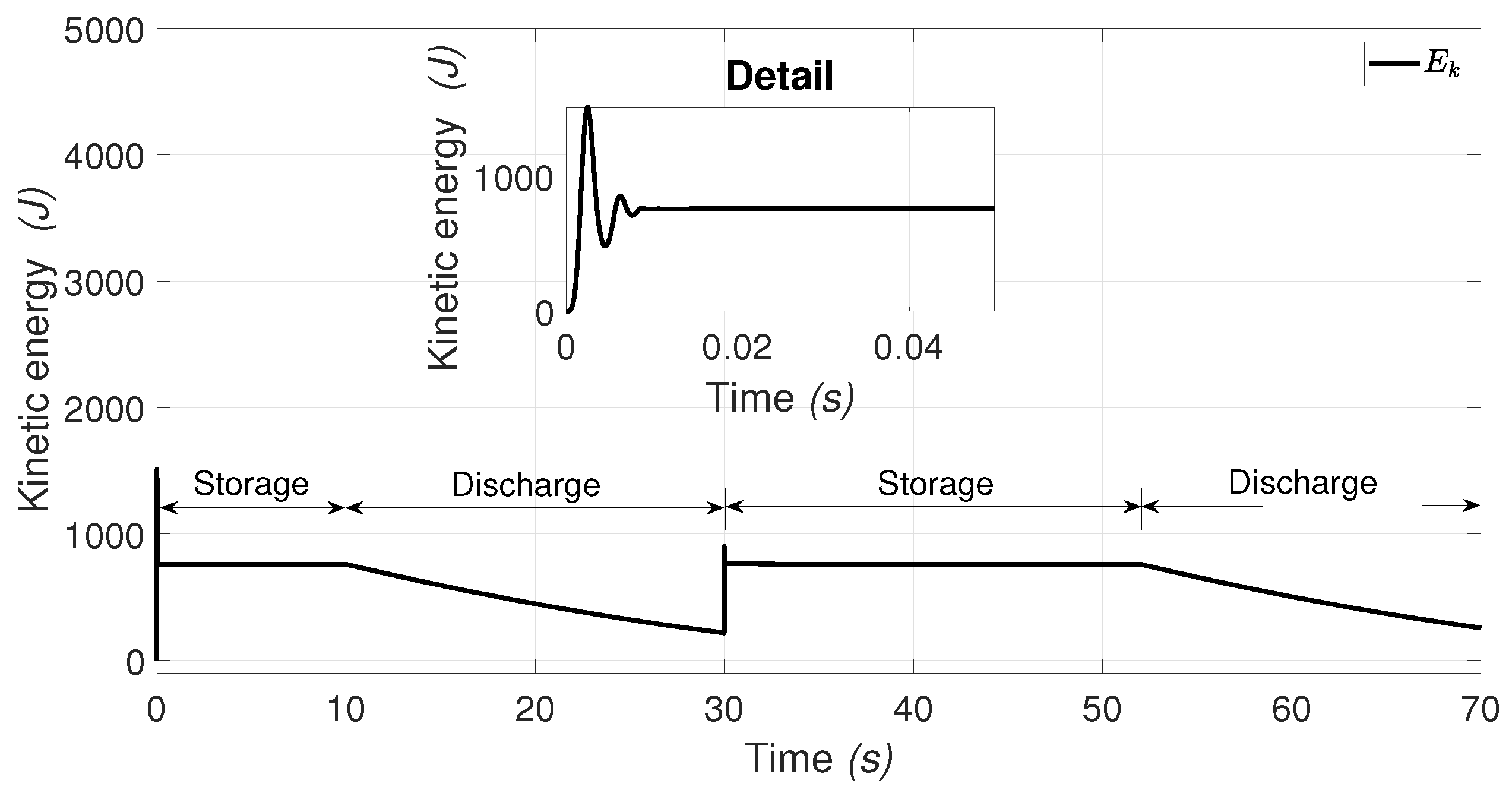
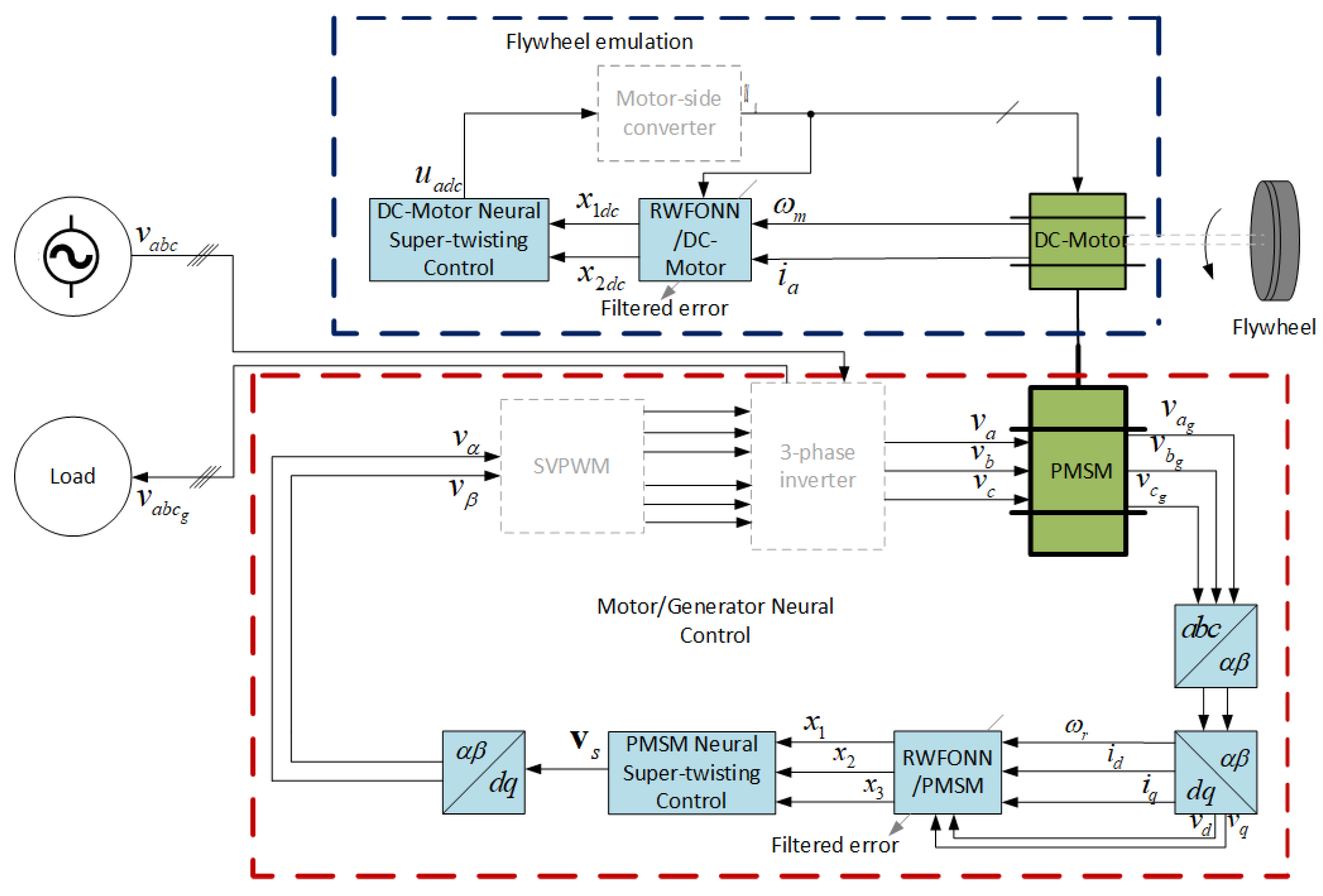
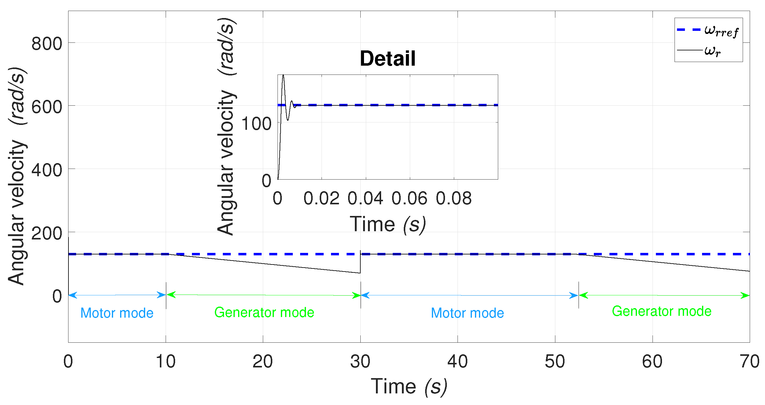
• The charging procedure (storing kinetic energy in the flywheel). This procedure consists of the PMSM in the $dq$ coordinate frame [30] working in motor mode to the control the angular velocity through the RWFONN using the block control linearization technique. In this scenario, the kinetic energy is stored in the flywheel (dotted red block in Figure 1);
• Discharging procedure (releasing energy). In this stage, the stored energy is now transferred to the PMSM working in generator mode. This scenario is considered in the case when there exists an electrical failure in the utility grid or when the flywheel is required to compensate with active power to the utility grid to solve a problem of the power management office, and the velocity controller for the DC-motor emulates the deceleration of the flywheel through the use of Equation (2). The flywheel energy discharge is emulated by the DC-machine (dotted blue block in Figure 1).

In this work, the sliding surface defined in Equation (8) is designed through the transformation of the RWFONN to the block controllable form involving the dynamics of the tracking error, such that this transformation resembles the structure described in Equation (7). By applying the super-twisting algorithm to the system (7) and using the RWFONN (Equation (5)), trained with the filtered error halgorithm (6), the result is the NSTC system, which is uniformly ultimately bounded (UUB). The stability proof is carried out in Appendix B.

Note that from Figure 1, the dotted blue block contains the motor-side converter gray block, where such block represents a future real-time implementation, while the dotted red block contains the gray blocks of the SVPWM and 3-phase inverter, which also represent a future real-time implementation.

Additionally, Figure 2 shows a general flowchart of the proposed algorithm applied to the control of both electrical machines, namely, the PMSM and the DC-motor. Both identification and control processes are indicated separately. Note that in this figure, there are particular notations for the PMSM (${\xi }_i$, $x_1$, ${\mathbf{u}}_{1s}$, and ${\epsilon }_1$) and for the DC-motor (${\xi }_{idc}$, $x_{1dc}$, $u_{sdc}$, and ${\zeta }_1$). The particular notations and the processes of identification and control will be explained in the following subsections.

3.1. Flywheel Storage System

In this section, the mathematical analysis of the stored kinetic energy from the flywheel, emulated by the DC-motor, is developed. Under the assumption that the mass is uniformly distributed and the axis of rotation passes through the mass center, the mass moment of inertia for a solid disk is given by [31]

$$\begin{array}{c}\hfill J_m=\frac{1}{2}m{r}^2,\end{array}$$

(11)

where $J_m$ is the mass moment of inertia and m, r are the mass and radius of the disk, respectively. Then, for the numerical calculation of the mass moment of inertia of the disk, when considering $m=2$ kg and $r=0.3$ m, Equation (11) yields

$$\begin{array}{c}\hfill J_m=0.09\mathrm{kg}·{\mathrm{m}}^2.\end{array}$$

(12)

Now, the kinetic energy storage equation is calculated when substituting Equation (12) into (1). Therefore, considering the angular velocity as ${\omega }_m=130$ rad/s, the energy stored in the flywheel results

$$E_k=760.5J$$

(13)

when considering that the deceleration caused by the kinetic energy stored in the flywheel is emulated by the DC-motor and its drive. To calculate the deceleration of the emulated flywheel, from the knowledge of the mass moment of inertia in Equation (12), replacing $J_m$ in Equation (2), it is then possible to calculate the reference angular velocity ${\omega }_{mref}$ for the DC-motor and, consequently, to be able to apply the NSTC.

3.2. Nonlinear Identification and NSTC Applied to PMSM

To convert the electrical energy applied to the PMSM into kinetic energy, the PMSM is activated in motor mode with the inputs $v_d$ and $v_q$. In the following subsections, the neural identification and the NSTC applied to the PMSM in motor mode are presented.

3.2.1. PMSM Neural Identification

In this work, the mathematical model of the PMSM is taken from [30], which consists of a third order nonlinear system given in the general form (3), which is modeled in a $dq$ coordinated frame rotating at the rotor velocity. Then, the RWFONN with structure (5), proposed to identify the dynamic system of the PMSM mathematical model, is defined as

$$\begin{array}{cc}\hfill {\dot{x}}_1=& -a_1{x}_1+b_1{w}_1{\psi }_1\left({\chi }_1\right)+x_2+x_3,\hfill \\ \hfill {\dot{x}}_2=& -a_2{x}_2+b_2{w}_2{\psi }_2\left({\chi }_2\right)+v_d,\hfill \\ \hfill {\dot{x}}_3=& -a_3{x}_3+b_3{w}_3{\psi }_3\left({\chi }_3\right)+v_q,\hfill \end{array}$$

(14)

where the RWFONN’s states $x_1$, $x_2$, and $x_3$ identify the states ${\omega }_r={\chi }_1$ (angular velocity), $i_d={\chi }_2$ (d-current), and $i_q={\chi }_3$ (q-current) from the PMSM, respectively. $a_1$, $a_2$, $a_3$, $b_1$, $b_2$, and $b_3$ are positive fixed parameters; $w_1$, $w_2$, $w_3$ are the synaptic weights; ${\psi }_1\left({\chi }_1\right)=e^{(-{\chi }_1^2/{\beta }_1)}\cos \left({\lambda }_1{\chi }_1\right)$, ${\psi }_2\left({\chi }_2\right)=e^{(-{\chi }_2^2/{\beta }_2)}\cos \left({\lambda }_2{\chi }_2\right)$, and ${\psi }_3\left({\chi }_3\right)=e^{(-{\chi }_3^2/{\beta }_3)}\cos \left({\lambda }_3{\chi }_3\right)$ are Morlet wavelet activation functions. The RWFONN’s inputs are the same as PMSM, $v_d$ and $v_q$. The filtered error algorithm used for training the RWFONN (Equation (14)) is performed as $w_1={\gamma }_1{\psi }_1\left({\chi }_1\right){\xi }_1$, $w_2={\gamma }_2{\psi }_2\left({\chi }_2\right){\xi }_2$ and $w_3={\gamma }_3{\psi }_3\left({\chi }_3\right){\xi }_3$, with ${\gamma }_1$, ${\gamma }_2$, ${\gamma }_3$ adjustable parameters, where ${\xi }_1=x_1-{\chi }_1$, ${\xi }_2=x_2-{\chi }_2$ and ${\xi }_3=x_3-{\chi }_3$ are the respective identification errors. According to Equation (5), $i=j=k=1,2,3$.

It should be noticed that the proposed structure (14) has only one neuron for each state, which represents a low computational burden in contrast with that from structures for high-order neural networks (HONNs). The parameters from the PMSM mathematical model are mentioned in [30], and the values are shown in

Table 1. Values and parameters of PMSM [32] and DC-motor [33].

PMSM Parameters	Value
Stator Resistance R	$1.4$$\Omega$
Inductance $L_d$	$6.6$ mH
Inductance $L_q$	$5.8$ mH
Inertial Moment J	$0.00176$ kg·m${}^2$
Damping Coefficient B	$0.00038818$ N·m ·s/rad
Flux Linkage ${\lambda }_{af}$	$0.1546$ V·s/rad
Pair Poles P	3
DC-motor Nameplate Data and Parameters	Value
Field Voltage	120 V
Field Current	$0.5$ A
Armature Voltage	120 V
Armature Current	$3.0$ A
Rotor Velocity	1750 rpm
Armature Resistance $R_a$	$12.5$$\Omega$
Armature Inductance $L_a$	$0.075$ H
Motor Constant $K_m$	$2.602$
Inertial Moment $J_m$	$0.0036$ N·m·s${}^2$
Frictional Coefficient $B_m$	$0.002$ N·m·s

[32].

3.2.2. NSTC Application to PMSM

In order to control the angular velocity ${\omega }_r$ of the PMSM, a first step toward that goal consists of transforming the RWFONN (Equation (14)) into the form (7) by using a recursive transformation of the tracking error ${\epsilon }_i$ [29]. For this, the structure of the system (14) is rewritten in the vector form

$$\begin{array}{cc}\hfill {\dot{x}}_1=& -a_1{x}_1+b_1{w}_1{\psi }_1\left({\chi }_1\right)+{\mathbf{a}}_1{\mathbf{x}}_2,\hfill \\ \hfill {\dot{\mathbf{x}}}_2=& {\mathbf{A}}_2{\mathbf{x}}_2+{\mathbf{A}}_3{\mathbf{b}}_1+{\mathbf{B}}_2\mathbf{v},\hfill \end{array}$$

(15)

with ${\mathbf{a}}_1=\left[\begin{array}{cc}1& 1\end{array}\right]$, ${\mathbf{A}}_2=\left[\begin{array}{cc}-a_2& 0\\ 0& -a_3\end{array}\right]$, ${\mathbf{A}}_3=\left[\begin{array}{cc}{b}_2{w}_2{\psi }_2\left({\chi }_2\right)& 0\\ 0& b_3{w}_3{\psi }_3\left({\chi }_3\right)\end{array}\right]$, ${\mathbf{b}}_1={\left[\begin{array}{cc}1& 1\end{array}\right]}^{\top }$, ${\mathbf{B}}_2=\left[\begin{array}{cc}1& 0\\ 0& 1\end{array}\right]$, ${\mathbf{x}}_2={\left[\begin{array}{cc}{x}_2& x_3\end{array}\right]}^{\top }$, and $\mathbf{v}={\left[\begin{array}{cc}{v}_d& v_q\end{array}\right]}^{\top }$. Now, by applying the recursive transformation to the structure (15) to resemble it into the block control form, the tracking error ${\epsilon }_1$ is defined by

$$\begin{array}{cc}\hfill {\epsilon }_1=& {\omega }_{rref}-x_1,\hfill \end{array}$$

(16)

where ${\omega }_{rref}$ is the reference angular velocity to the PMSM, and $x_1$ represents the state of the neural network (15). Therefore, the tracking error dynamics are given as

$$\begin{array}{cc}\hfill {\dot{\epsilon }}_1=& {\dot{\omega }}_{rref}-{\dot{x}}_1.\hfill \end{array}$$

(17)

Substituting ${\dot{x}}_1$ Equation (15) into (17), and assigning the desired dynamics $k_1{\epsilon }_1$, it yields

$$\begin{array}{cc}\hfill {\dot{\epsilon }}_1=& {\dot{\omega }}_{rref}-(-a_1{x}_1+b_1{w}_1{\psi }_1\left({\chi }_1\right)+{\mathbf{a}}_1{\mathbf{x}}_2)=-k_1{\epsilon }_1,\hfill \end{array}$$

(18)

where $k_1$ is adjusted to vanish the tracking error. In this way, it is possible to synthesize a control law through the vector state ${\mathbf{x}}_2$, where the reference vector is defined as

$$\begin{array}{c}\hfill {\mathbf{x}}_{2ref}={\mathbf{a}}_1^{\mathrm{pinv}}[{\dot{\omega }}_{rref}+a_1{\omega }_{rref}-a_1{\epsilon }_1-b_1{w}_1{\psi }_1\left({\chi }_1\right)+k_1{\epsilon }_1],\end{array}$$

(19)

where the superscript “pinv” denotes the pseudo-inverse. Furthermore, the second error in vector form is defined as

$$\begin{array}{c}\hfill {\epsilon }_2={\mathbf{x}}_{2ref}-{\mathbf{x}}_2\end{array}$$

(20)

with dynamics

$$\begin{array}{cc}\hfill {\dot{\epsilon }}_2=& {\dot{\mathbf{x}}}_{2ref}-{\dot{\mathbf{x}}}_2.\hfill \end{array}$$

(21)

Substituting Equation (15) into (21) yields

$$\begin{array}{cc}\hfill {\dot{\epsilon }}_2=& {\dot{\mathbf{x}}}_{2ref}-{\mathbf{A}}_2{\mathbf{x}}_{2ref}+{\mathbf{A}}_2{\epsilon }_2-{\mathbf{A}}_3{\mathbf{b}}_1-{\mathbf{B}}_2\mathbf{v}.\hfill \end{array}$$

(22)

Moreover, using Equations (18) and (22), the representation in the block control form from Equation (15), in terms of the tracking error ${\epsilon }_i$, is obtained as

$$\begin{array}{cc}\hfill {\dot{\epsilon }}_1=& -k_1{\epsilon }_1+{\mathbf{a}}_1{\epsilon }_2,\hfill \\ \hfill {\dot{\epsilon }}_2=& {\mathbf{a}}_1^{\mathrm{pinv}}[{\ddot{\omega }}_{rref}+a_1{\dot{\omega }}_{rref}-b_1{w}_1{\psi }_1\left({\chi }_1\right)]\hfill \\ & -{\mathbf{A}}_2\left({\mathbf{a}}_1^{\mathrm{pinv}}[{\ddot{\omega }}_{rref}+a_1{\dot{\omega }}_{rref}-b_1{w}_1{\psi }_1\left({\chi }_1\right)]\right)\hfill \\ & +0.5\left[\begin{array}{c}{a}_1{k}_1-k_1^2+a_1{a}_2{k}_1-a_2{k}_1^2\\ a_1{k}_1-k_1^2+a_1{a}_3{k}_1-a_3{k}_1^2\end{array}\right]{\epsilon }_1+{\mathbf{A}}_2{\epsilon }_2-{\mathbf{A}}_3{\mathbf{b}}_1-{\mathbf{B}}_2\mathbf{v},\hfill \end{array}$$

(23)

Furthermore, defining the sliding surface $s={\epsilon }_2$, with the relative degree from Equation (23) equals to 1, and applying the NSTC Equation (9) in (23) results

$$\begin{array}{cc}\hfill {\dot{\epsilon }}_1=& -k_1{\epsilon }_1+{\mathbf{a}}_1{\epsilon }_2,\hfill \\ \hfill {\dot{\epsilon }}_2=& {\mathbf{a}}_1^{\mathrm{pinv}}[{\ddot{\omega }}_{rref}+a_1{\dot{\omega }}_{rref}-b_1{w}_1{\psi }_1\left({\chi }_1\right)]\hfill \\ & -{\mathbf{A}}_2\left({\mathbf{a}}_1^{\mathrm{pinv}}[{\ddot{\omega }}_{rref}+a_1{\dot{\omega }}_{rref}-b_1{w}_1{\psi }_1\left({\chi }_1\right)]\right)\hfill \\ & +0.5\left[\begin{array}{c}{a}_1{k}_1-k_1^2+a_1{a}_2{k}_1-a_2{k}_1^2\\ a_1{k}_1-k_1^2+a_1{a}_3{k}_1-a_3{k}_1^2\end{array}\right]{\epsilon }_1+{\mathbf{A}}_2{\epsilon }_2-{\mathbf{A}}_3{\mathbf{b}}_1-{\mathbf{B}}_2({\lambda }_s{\left|\mathbf{s}\right|}^{\frac{1}{2}}\mathrm{sign}\left(\mathbf{s}\right)+{\mathbf{u}}_{1s}),\hfill \end{array}$$

(24)

where ${\mathbf{u}}_{1s}$ represents the control vector. Note that in Equation (23), the control input vector $\mathbf{v}={\left[v_d{v}_q\right]}^{\top }$ is replaced by the STC resulting Equation (24) under the fact that the tracking error variables ${\epsilon }_1$ and ${\epsilon }_2$ are decoupled. This latter will guarantee that the tracking errors be steered to zero in finite time. From Equation (24), selecting the sliding surface $\mathbf{s}=x_2$ arises the system given by [29]

$$\begin{array}{cc}\hfill \dot{\mathbf{s}}=& {\mathbf{a}}_1^{\mathrm{pinv}}[{\ddot{\omega }}_{rref}+a_1{\dot{\omega }}_{rref}-b_1{w}_1{\psi }_1\left({\chi }_1\right)]\hfill \\ & -{\mathbf{A}}_2\left({\mathbf{a}}_1^{\mathrm{pinv}}[{\ddot{\omega }}_{rref}+a_1{\dot{\omega }}_{rref}-b_1{w}_1{\psi }_1\left({\chi }_1\right)]\right)\hfill \\ & +0.5\left[\begin{array}{c}{a}_1{k}_1-k_1^2+a_1{a}_2{k}_1-a_2{k}_1^2\\ a_1{k}_1-k_1^2+a_1{a}_3{k}_1-a_3{k}_1^2\end{array}\right]{\epsilon }_1+{\mathbf{A}}_2{\epsilon }_2-{\mathbf{A}}_3{\mathbf{b}}_1-{\mathbf{B}}_2({\lambda }_s{\left|\mathbf{s}\right|}^{\frac{1}{2}}\mathrm{sign}\left(\mathbf{s}\right)+{\mathbf{u}}_{1s}),\hfill \\ \hfill {\dot{\mathbf{u}}}_{1s}=& {\alpha }_s\mathrm{sign}\left(\mathbf{s}\right).\hfill \end{array}$$

(25)

where Equation (25) is the NSTC applied to the PMSM through the RWFONN structure.

3.3. Nonlinear Identification and NSTC Applied to DC-Motor

In order to convert the kinetic energy stored by the flywheel into electrical energy, the PMSM must be operated in generator mode. The discharge of the kinetic energy is controlled by the angular velocity of the DC-motor, this can be achieved by decelerating the angular velocity taking into account the reference velocity generated by Equation (2).

3.3.1. DC-Motor Neural Identification

The mathematical model of the DC-motor is taken from [16], which consists of a three state nonlinear system with structure (3). Note that due to the linearity between the effective field current and its constant magnetizing flux, the mathematical model of the DC-motor becomes a linear system of two differential equations. Therefore, the RWFONN here proposed, following the structure (5), to identify the dynamics of the DC-motor mathematical model is defined as

$$\begin{array}{cc}\hfill {\dot{x}}_{1dc}=& -a_{1dc}{x}_{1dc}+b_{1dc}{w}_{1dc}{\psi }_{1dc}\left({\chi }_{1dc}\right)+x_{2dc},\hfill \\ \hfill {\dot{x}}_{2dc}=& -a_{2dc}{x}_{2dc}+b_{2dc}{w}_{2dc}{\psi }_{2dc}\left({\chi }_{2dc}\right)+u_{adc},\hfill \end{array}$$

(26)

where the RWFONN’s states $x_{1dc}$ and $x_{2dc}$ identify the states ${\omega }_m={\chi }_{1dc}$ (angular velocity) and $i_a={\chi }_{2dc}$ (armature current) from the DC-motor, respectively. $a_{1dc}$, $a_{2dc}$, $b_{1dc}$, and $b_{2dc}$ are positive constant parameters; $w_{1dc}$ and $w_{2dc}$ are the synaptic weights; ${\psi }_{1dc}\left({\chi }_{1dc}\right)=e^{(-{\chi }_{1dc}^2/{\beta }_{1dc})}\cos \left({\lambda }_{1dc}{\chi }_{1dc}\right)$ and ${\psi }_{2dc}\left({\chi }_{2dc}\right)=e^{(-{\chi }_{2dc}^2/{\beta }_{2dc})}\cos \left({\lambda }_{2dc}{\chi }_{2dc}\right)$ are Morlet wavelet activation functions. The RWFONN’s input $u_{adc}$ is the same as $u_a$ (armature voltage) to the DC-motor. The filtered error algorithm used for training the RWFONN (Equation (26)) is performed through $w_{1dc}={\gamma }_{1dc}{\psi }_{1dc}\left({\chi }_{1dc}\right){\xi }_{1dc}$ and $w_{2dc}={\gamma }_{2dc}{\psi }_{2dc}\left({\chi }_{2dc}\right){\xi }_{2dc}$ with ${\gamma }_{1dc}$, ${\gamma }_{2dc}$ adjustable parameters, and ${\xi }_{1dc}=x_{1dc}-{\chi }_{1dc}$, ${\xi }_{2dc}=x_{2dc}-{\chi }_{2dc}$ are the respective identification errors. From Equation (5), $i=j=k=1,2$.

It must be noticed that the proposed RWFONN (Equation (26)) has only one neuron for each state, in a similar way as in Equation (14), which represents a low computational burden in contrast with HONN. The parameters of the DC-motor mathematical model are mentioned in [16], whose values are shown in Table 1.

3.3.2. NSTC Application to DC-Motor

By following the methodology as that in Section 3.2.2, the recursive transformation is now applied to the structure (26), where the generation of the tracking error ${\zeta }_1$ is defined by

$$\begin{array}{c}\hfill {\zeta }_1={\omega }_{mref}-x_{1dc}\end{array}$$

(27)

where ${\omega }_{mref}$ represents the reference angular velocity of the DC-motor and $x_{1dc}$ is the state variable from Equation (26). The dynamics of the tracking error ${\zeta }_1$ is given by

$$\begin{array}{c}\hfill {\dot{\zeta }}_1={\dot{\omega }}_{mref}-{\dot{x}}_{1dc}.\end{array}$$

(28)

By substituting Equation (26) into (28) yields

$$\begin{array}{cc}\hfill {\dot{\zeta }}_1=& {\dot{\omega }}_{mref}-(-a_{1dc}{x}_{1dc}+b_{1dc}{w}_{1dc}{\psi }_{1dc}\left({\chi }_{1dc}\right)+x_{2dc})=-k_{1dc}{\zeta }_1,\hfill \end{array}$$

(29)

where $k_{1dc}{\zeta }_1$ constitutes the desired dynamics to vanish the tracking error. In this way, it is possible to synthesize a control law through the state $x_{2dc}$, so, to such an end consider

$$\begin{array}{cc}\hfill x_{2dcref}=& {\dot{\omega }}_{mref}+a_{1dc}{\omega }_{mref}-a_{1dc}{\zeta }_1-b_{1dc}{w}_{1dc}{\psi }_{1dc}\left({\chi }_{1dc}\right)+k_{1dc}{\zeta }_1.\hfill \end{array}$$

(30)

Furthermore, the second error is defined as

$$\begin{array}{c}\hfill {\zeta }_2=x_{2dcref}-x_{2dc},\end{array}$$

(31)

with error dynamics

$$\begin{array}{c}\hfill {\dot{\zeta }}_2={\dot{x}}_{2dcref}-{\dot{x}}_{2dc}.\end{array}$$

(32)

By substituting Equation (26) in (32) it yields

$$\begin{array}{c}\hfill {\dot{\zeta }}_2={\dot{x}}_{2dcref}-(-a_{2dc}{x}_{2dc}+b_{2dc}{w}_{2dc}{\psi }_{2dc}\left({\chi }_{2dc}\right)+u_{adc}).\end{array}$$

(33)

Moreover, using Equations (29) and (33), the block control form for Equation (26) is defined as

$$\begin{array}{cc}\hfill {\dot{\zeta }}_1=& -k_{1dc}{\zeta }_1+{\zeta }_2,\hfill \\ \hfill {\dot{\zeta }}_2=& {\dot{x}}_{2dcref}+a_{2dc}{x}_{2dc}-b_{2dc}{w}_{2dc}{\psi }_{2dc}\left({\chi }_{2dc}\right)-u_{adc}.\hfill \end{array}$$

(34)

Thus, based on the error dynamics ${\zeta }_i$, the Equation (34) represents the block control transformation with structure (26). Furthermore, from the system (26) with relative degree equals to 1, the NSTC is given by

$$\begin{array}{cc}\hfill {\dot{\zeta }}_1=& -k_{1dc}{\zeta }_1+{\zeta }_2,\hfill \\ \hfill \dot{{\zeta }_2}=& {\ddot{\omega }}_{mref}+(-a_{1dc}+a_{2dc}){\dot{\omega }}_{mref}+\left(a_{1dc}{a}_{2dc}\right){\omega }_{mref}\hfill \\ & -(a_{1dc}{k}_{1dc}+k_1^2+a_{1dc}{a}_{2dc}-a_{2dc}{k}_{1dc}){\zeta }_1-a_{2dc}{\zeta }_2-a_{2dc}{b}_{1dc}{w}_{1dc}{\psi }_{1dc}\left({\chi }_{1dc}\right)-\hfill \\ & b_{2dc}{w}_{2dc}{\psi }_{2dc}\left({\chi }_{2dc}\right)-({\lambda }_{sdc}|s_{dc}{|}^{\frac{1}{2}}\mathrm{sign}\left(s_{dc}\right)+u_{sdc})\hfill \end{array}$$

(35)

It should be noticed from Equation (35), regarding the tracking error variables ${\zeta }_1$ and ${\zeta }_2$, that the control input $u_{sdc}=u_{adc}$ guarantees that these errors will be steered to zero in finite time.

4. Simulation Results

This work presents the simulation results of the NSTC for controlling the angular velocity of a PMSM and a DC-motor to emulate an FESS. The angular velocity of the PMSM is controlled to store kinetic energy in the flywheel, meanwhile the angular velocity of the DC-machine is controlled to emulate the deceleration of the flywheel by transferring kinetic energy to the PMSM working in generator mode, where it is converted into electrical energy and delivered to the utility grid. The used parameters of the motors are shown in Table 1. The simulation was performed using Matlab/Simulink ($Matla{b}^{TM}$) with a Runge–Kutta solver and a step size of 100 μs.

4.1. Neural Identification

This subsection presents the simulation results of the neural identification of the PMSM state variables, as well as the DC-motor state variables using the RWFONN structure.

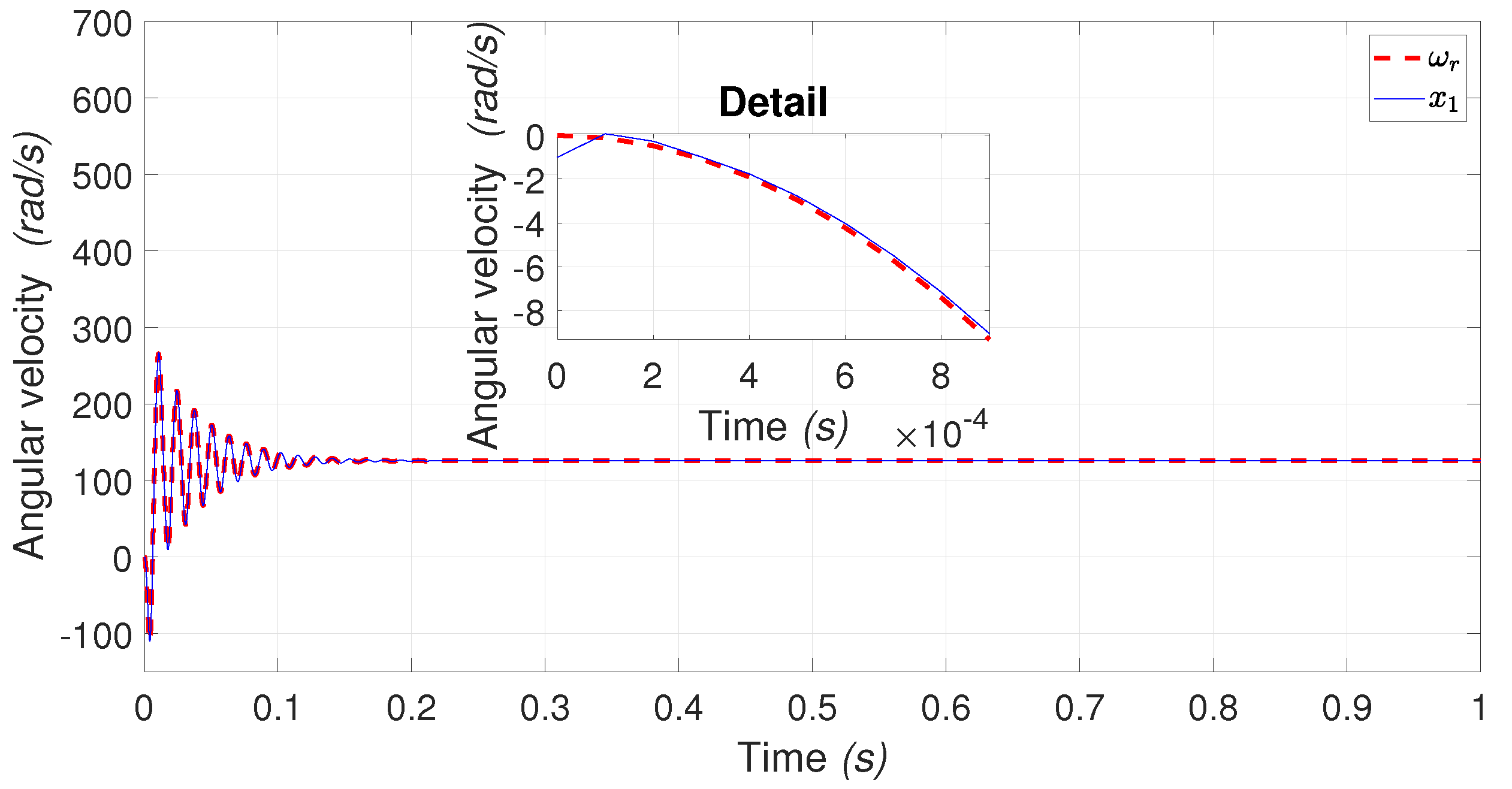
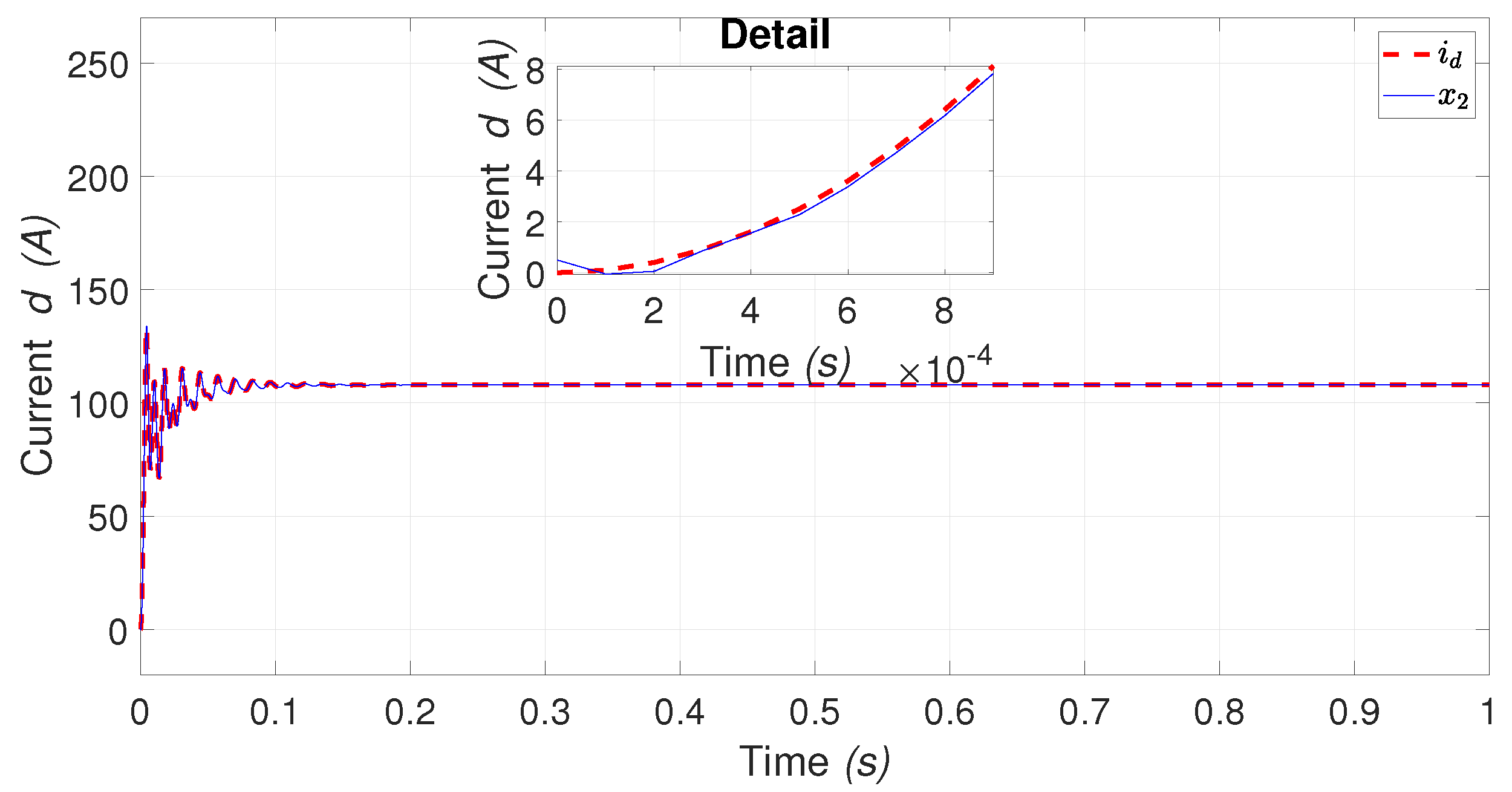
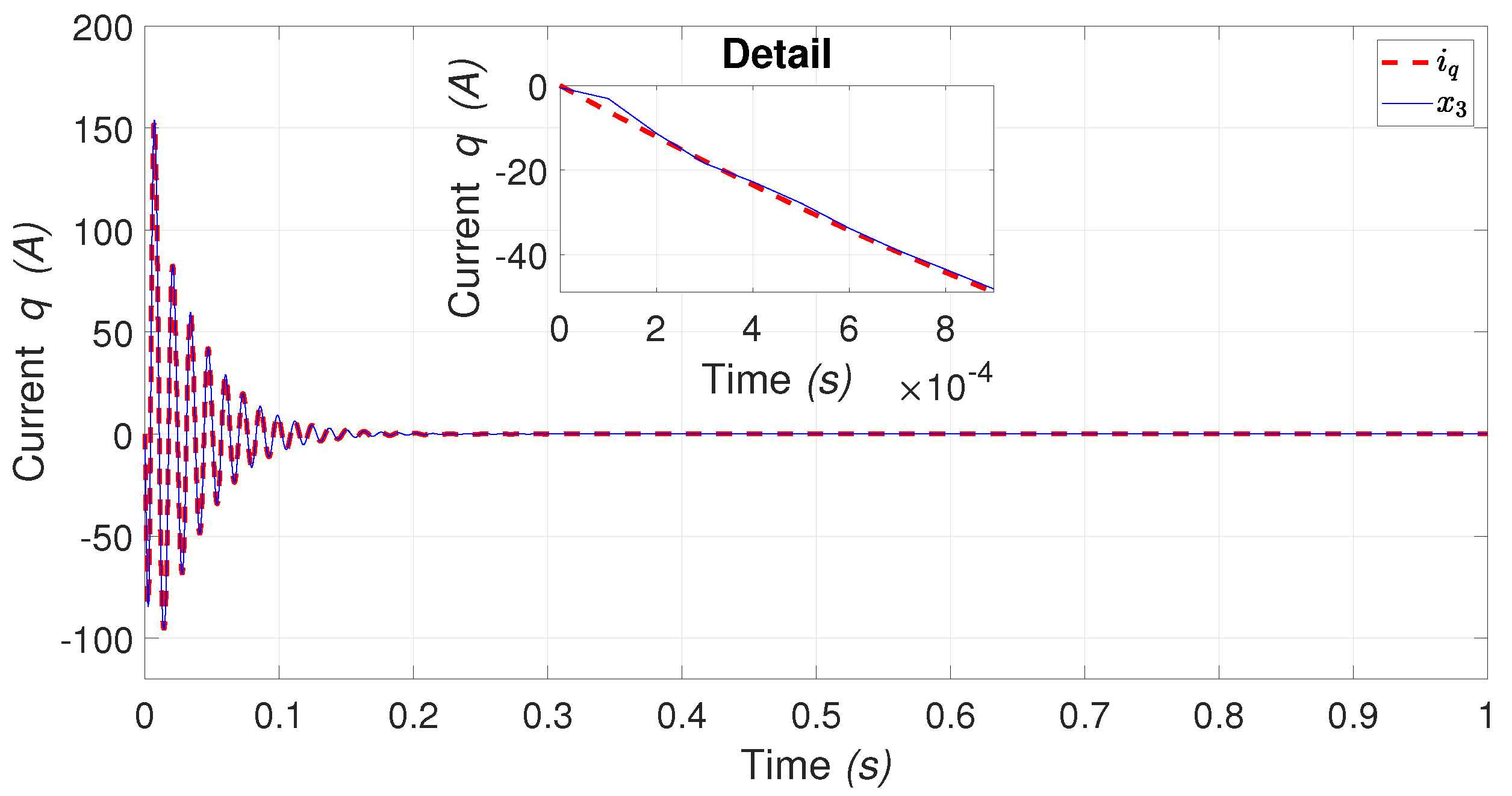
4.1.1. PMSM States Identification

For the neural identification of the PMSM states, the parameter values are: $a_1=6000$, $a_2=a_3=4000$ and $b_1=6000$, $b_2=b_3=4000$; the parameters for the Morlet Wavelet activation functions are: ${\beta }_1=75\times {10}^3$, ${\beta }_2=22\times {10}^3$, ${\beta }_3=35\times {10}^3$, ${\lambda }_1={\lambda }_2={\lambda }_3=0.001$; the parameters of the filtered error are: ${\gamma }_1={\gamma }_2={\gamma }_3=855\times {10}^2$. In Figure 3, Figure 4 and Figure 5, the neuronal identification of the PMSM states is shown, where, in Figure 3 the identification of the angular velocity is the red dashed line that represents the angular velocity of the PMSM (${\omega }_r$) and the blue continuous line represents the state of RWFONN ($x_1$). In order to show the convergence of these results, the initial conditions are given as: ${\omega }_r=0$ and $x_1=-1$. Note that in the detail of the figure, the identification convergence is given in $0.0002$ s, approximately. The transient is shown when the PMSM is started in the energy storage, where the velocity response has a settling time of 0.15 s, approximately.

The identification of current $i_d$ is presented in Figure 4, where the red dashed line represents the current of the PMSM ($i_d$) and the blue continuous line represents the state of RWFONN ($x_2$); the initial conditions are given as: $i_d=0$ and $x_2=0.5$. The identification convergence is given in $0.0003$ s approximately, as is shown in the detail of the Figure 4. In the transient response, the inrush current $i_d$ achieves a maximum value of the 132 A with an oscillation frequency of 0.0014 Hz. As it is shown, the identification process is effectively realized.

In Figure 5 the identification of current q is shown, where the red dashed line represents the current $i_q$ of the PMSM, and the blue continuous line represents the state of the RWFONN ($x_3$), and where the initial conditions are given as: $i_q=0$ and $x_3=-0.5$. The identification convergence is given in $0.0003$ s, approximately. Figure 5 shows the transient when the PMSM is started, and in the process of energy storage, the inrush current $i_q$ achieves a maximum value of the 153 A with an oscillation frequency of 0.0489 Hz. In the transient, the identification procedure is more demanding and is effectively realized.

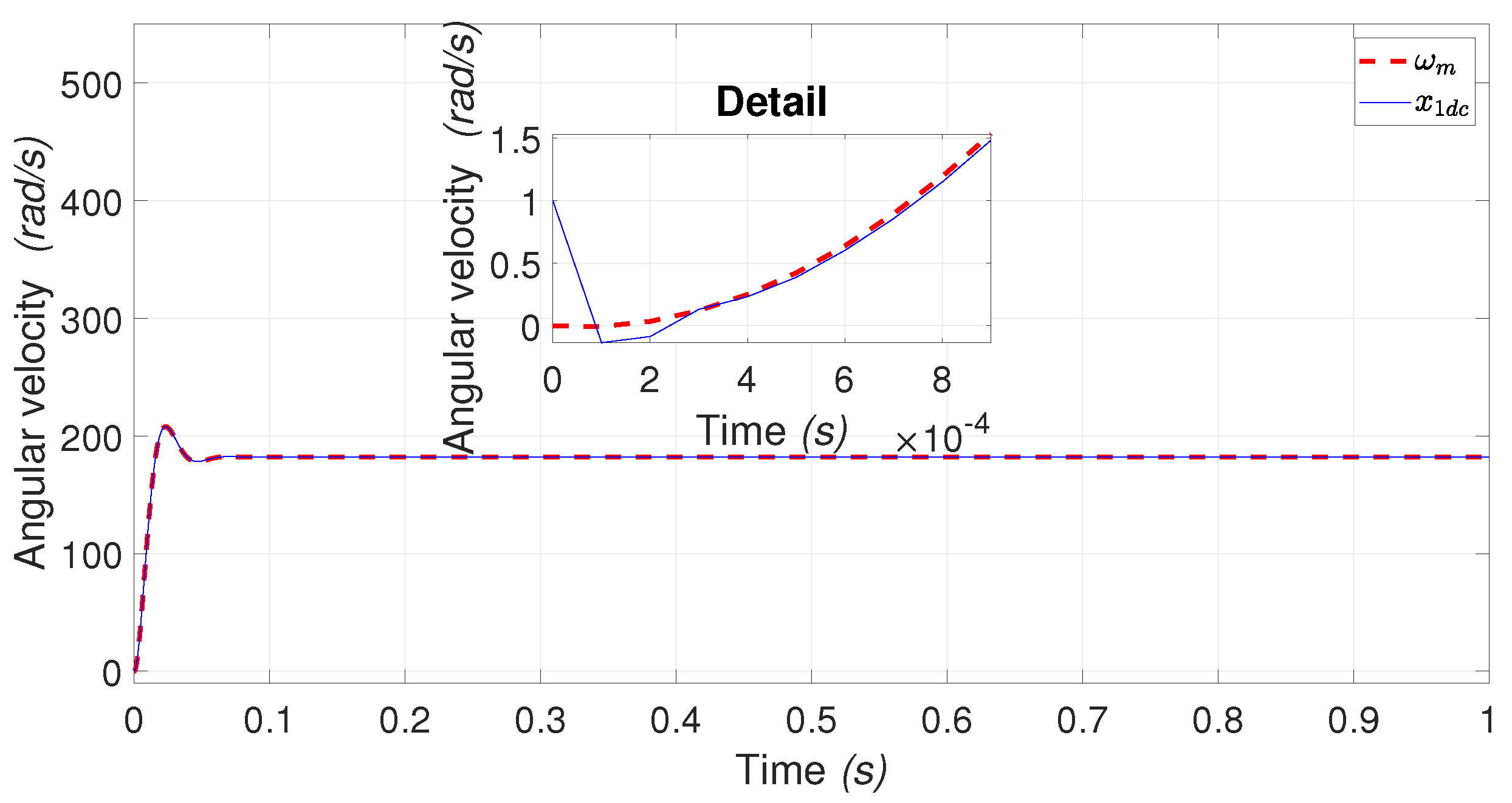
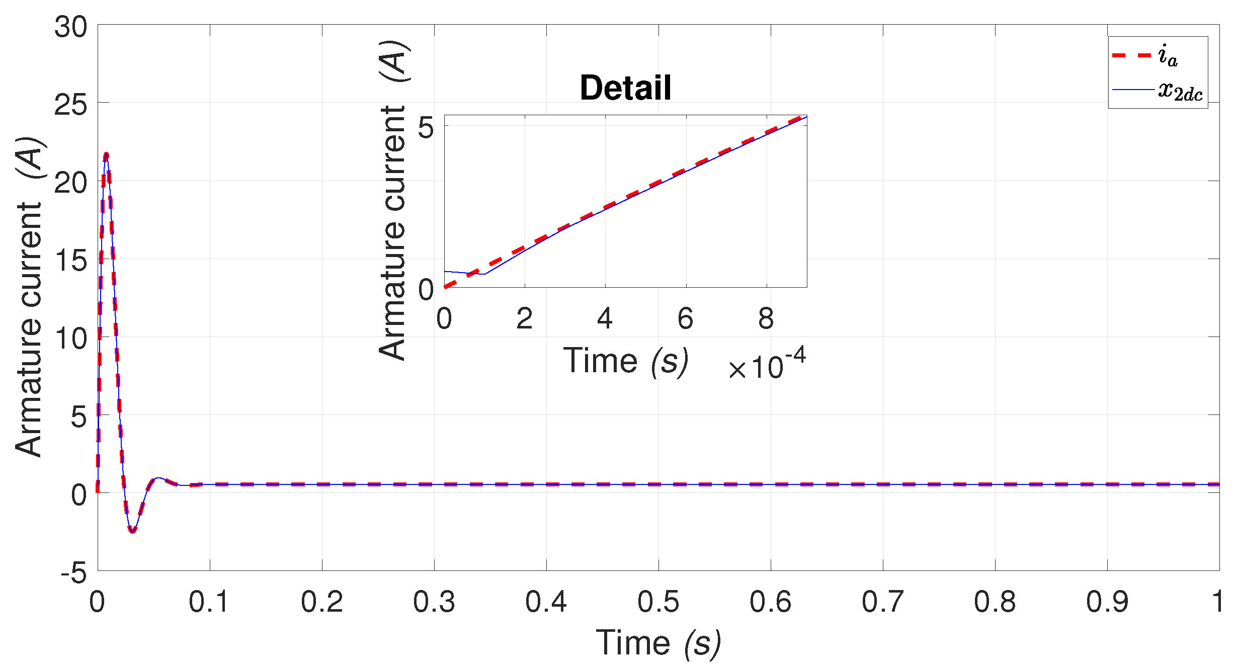
4.1.2. DC-motor States Identification

In this section, the neuronal identification of the DC-motor states is carried out, where the values of the parameters used in the RWFONN are defined as follows: $a_{1dc}=a_{2dc}=6000$ and $b_{1dc}=b_{2dc}=6000$; the parameters for the Morlet Wavelet activation functions are: ${\beta }_{1dc}=85\times {10}^3$, ${\beta }_{2dc}=75\times {10}^3$, ${\lambda }_{1dc}=0.001$, ${\lambda }_{2dc}=0.01$; the parameters of the filtered error are: ${\gamma }_{1dc}={\gamma }_{2dc}=855\times {10}^2$.

In Figure 6, the neural identification of the angular velocity of the DC-motor is shown. In this figure, ${\omega }_m$ is a state variable of the motor, and $x_{1dc}$ is a state variable of the NN. As it can be seen in the detail of the figure, the NN identifies the state of the motor with a convergence time of $0.0003$ s. The initial conditions are: ${\omega }_m=0$ and $x_{1dc}=1$. The figure shows the transient when the DC-motor is starting. The velocity response in the transient has an overshoot of $1.13\%$ and a settling time of 0.05 s.

Figure 7 shows the neural identification of the armature current of DC-motor, where $i_a$ is the current of the motor and $x_{2dc}$ is the state of the network; the initial conditions are: $i_a=0$ and $x_{2dc}=0.5$, and obtaining the neural identification with a time of convergence $0.0004$ s, approximately. In this figure, the transient presents the typical inrush current of a DC-motor when it is fed with nominal voltage. The current has a maximum value of 21.7 A and achieves the steady-state value of 0.53 A at 0.08 s.

In order to make a comparison of the performance of the RWFONN used in this work, numerical simulation results about the identification process from both Recurrent Sigmoid First-Order Neural Network (RSFONN) and RHONN have been obtained. This comparison consists of using the RHONN and RSFONN structures, instead of that for the RWFONN, to the dynamics identification of the plant, training them via a filtered error algorithm. Then, from the data obtained by the identification process, the root mean square (RMS) error is computed, which represents the difference between the actual state and the estimated state when using approaches with different NNs. The comparison is made by estimating the states from both PMSM and DC-motor, where

Table 2. RMS error for PMSM.

Neural Network Structure	${\mathit{\omega }}_{\mathit{r}}$	${\mathit{i}}_{\mathit{d}}$	${\mathit{i}}_{\mathit{q}}$
RWFONN	0.1496	0.0311	0.0263
RSFONN	0.0105	0.0015	0.0286
RHONN	0.0386	0.0032	0.0128

and

Table 3. RMS error for DC-motor.

Neural Network Structure	${\mathit{\omega }}_{\mathit{m}}$	${\mathit{i}}_{\mathit{a}}$
RWFONN	0.0018	0.00004
RSFONN	0.0004	0.00005
RHONN	0.0206	0.0009

show the RMS for each state from both motors, respectively. It can be seen in Table 2 that the lowest RMS values (bold values) are for ${\omega }_r$ and $i_d$ from the RSFONN and for $i_q$ from the RHONN. In Table 3, the results show that the lowest RMS values (bold values) are for ${\omega }_m$ from the RSFONN and for $i_a$ from the RWFONN.

Even when different NNs obtain the lowest RMS in the identification process, there are different reasons to consider when choosing the NN structure. Such is the case with the RWFONN, having a very single structure, for which it is easy to apply the STA, contrary to the case with the RHONN or even the RSFONN. Another important thing is that the computational burden is lower for simple structures such as the RWFONN but not for the RHONN or when increasing the high-order terms of the latter.

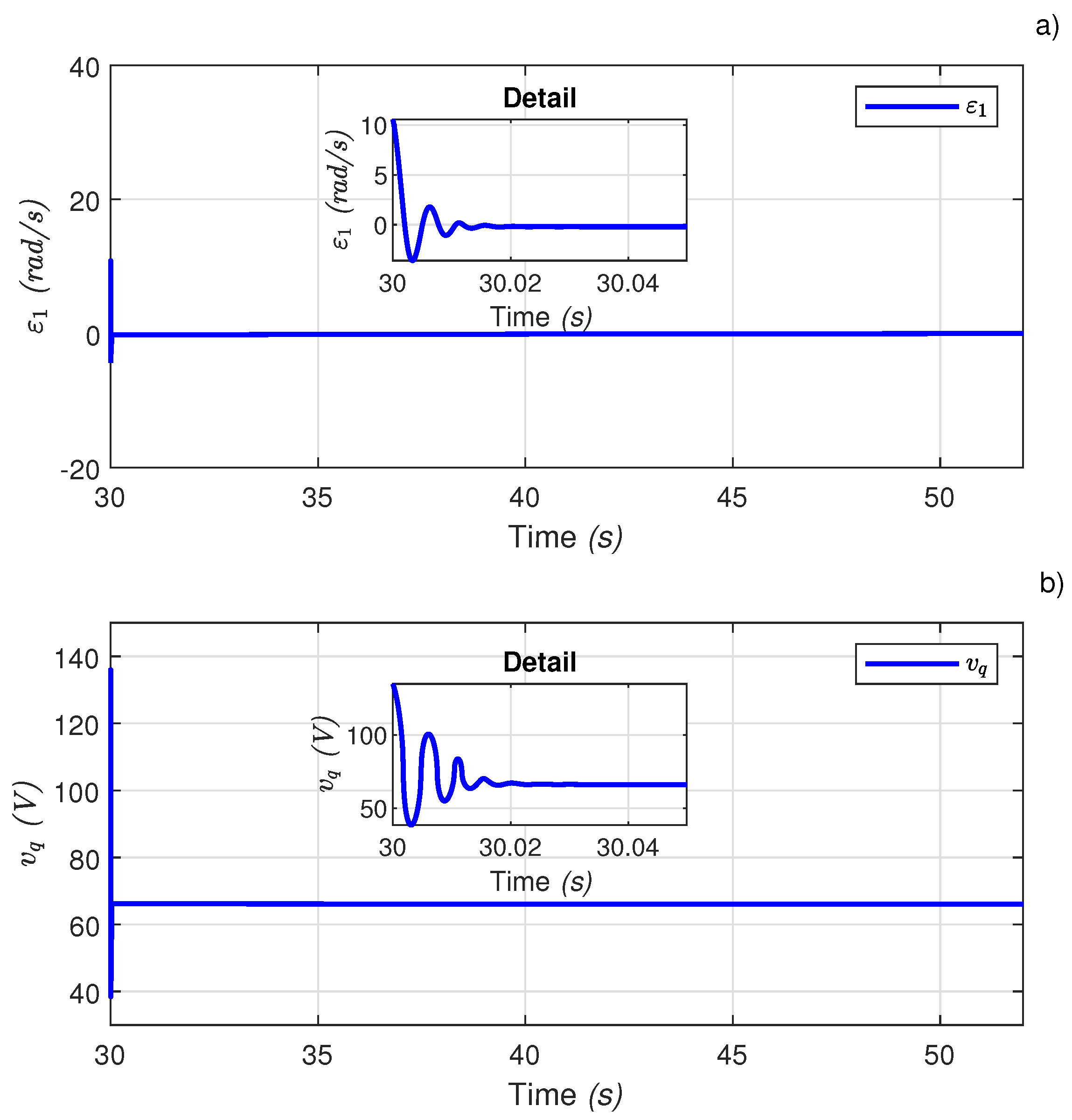
4.2. PMSM and DC-motor Controller-Emulation of Flywheel

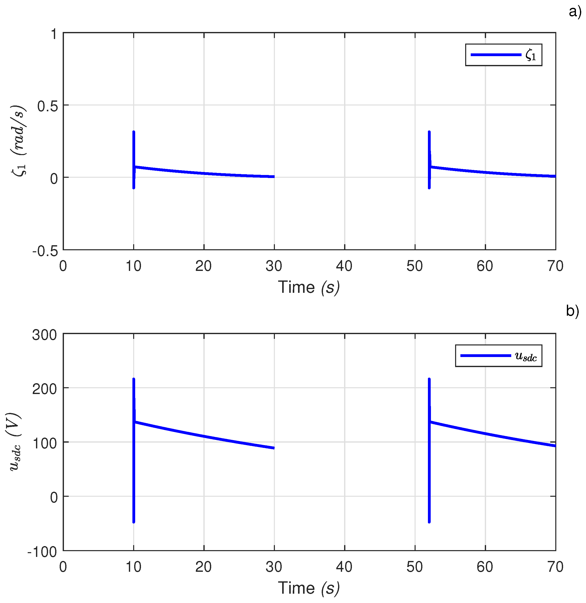
In this subsection, the NSTC for PMSM and a DC-motor controller for emulating the complete system of the flywheel are presented. For the case of the PMSM, the controller is designed to control the angular velocity (${\omega }_m$) indirectly through the states of the NN, where the parameters and gains for the NSTC of PMSM are defined as: $k_1=8000$, ${\lambda }_{1s}=0.1$, ${\lambda }_{2s}=2.5$, and ${\alpha }_{1s}=0.1$, ${\alpha }_{2s}=2.5$.

In Figure 8, the behavior of the PMSM in motor and generator modes is shown. In the case of motor mode, the velocity tracking performances from 0 to 10 and from 30 to 52 s are shown, where the blue dashed line represents ${\omega }_{rref}$, and black continuous line is ${\omega }_m$. In this time, the tracking is to ${\omega }_{rref}=130$ rad/s, and there is kinetic energy storage during this operation mode. A detail of the transient is shown where a fast convergence can be seen. Due to consideration of a grid failure, the case of PMSM as a generator mode is plotted during the period of time from 10 to 30 and from 52 to 70 s. In this time, the deceleration of the flywheel is emulated by controlling the angular velocity of the DC-motor (see Figure 9 on the sign named Discharge of flywheel) and in this figure, the velocity reference ${\omega }_{mref}$ (blue dashed line) is described by Equation (2) and meanwhile, ${\omega }_m$ is the gray continuous line; a detail is shown in the middle of the figure where the very good results of the tracking can be noted. To ensure the NSTC of the DC-motor, the parameters and gains are defined as: $k_{1dc}=8000$, ${\lambda }_{sdc}=3$ and ${\alpha }_{sdc}=3$.

Figure 10 shows the PMSM velocity controller performance, where tracking velocity error ${\epsilon }_1$ (Figure 10a) is steered to zero effectively by the super-twisting control law $v_q$ (Figure 10a). Note that the transient response at 30 s corresponds to the change from the generator to motor mode. The error diminishes to zero in 0.015 s, as can be seen in the detail of Figure 10a.

Figure 11 shows the DC-motor velocity controller performance. Figure 11a displays the tracking error signal in the intervals (10–30 s) and (52–70 s), which is steered to zero in finite time by the action of the super-twisting control law shown in Figure 11b. When the tracking error is zero, then the velocity control of the DC-motor is achieved, and the control goal is fulfilled, which consists of emulating the deceleration of the flywheel.

4.3. Power Delivery

In Figure 12, the kinetic energy stored in the flywheel is shown from 0 to 10 s and from 30 to 52 s due to the fact that PMSM is in motor mode, generating 760.5 J in steady-state. From 10 to 30 s and from 52 to 70 s, the PMSM is in generator mode, and it shows the discharge of the energy when considering a fault in the utility grid or when the flywheel is required to compensate for the utility grid with active power to solve a problem of the electrical office.

5. Discussion

There exists a variety of three-phase electrical machines that can be implemented in an FESS, such as wound squirrel cage [34] and doubly-fed asynchronous machines [35]. In this work, we used the PMSM to emulate a flywheel storage system because, based on the literature, the small and medium capacity applications of the flywheels make it more convenient to use the PMSM since it is more efficient and less difficult to control. The doubly-fed induction generator is used more in large capacities because the control is carried out by the rotor circuit, where the power flow is proportional to the slip of the machine. Consequently, the electronic power drive is of lower capacity, near 30% of the flywheel capacity, which allows a considerable economic saving in the converter.

This proposal can be extended to other applications in energy storage systems such as power compensators in wind generators as well as wind diesel power systems, electric vehicles, direct electrical grid applications, i.e., applications where it is possible to involve charge/discharge cycles.

Regarding the advantages, this work can be used as a general methodology where it is possible to work as a motor/generator, such as wound squirrel cage, doubly fed asynchronous machines, and of course the PMSM. It is clear that this is possible by making the corresponding changes for the mathematical model of the machine to be used, which all depends on the range of speeds that it is going to operate at, and taking advantage of the benefits offered by the material with which the machine is built (low-speed FESS, or high-speed FESS [35]), and the particular features (electrical, mechanical) of the three-phase machine, etc. It is possible to control nonlinear and linear systems using the NSTC based on RWFONNs trained via a filtered error algorithm. These plants to be controlled are considered unknown regarding the parameters, and only the state-space variables are measured. This work can be extended to other three-phase machines, such as doubly fed asynchronous machines or wound squirrel cage motors.

The main limitation is that this work is an emulated system in simulation, and even when different real scenarios are considered, a real system will always show all the benefits of the proposal. Furthermore, this work is limited by the structure of the RWFONN, as even when the obtained numerical results are good, the computational process can be degraded.

The following interpretation of the results are made: the identification (Figure 3, Figure 4, Figure 5, Figure 6 and Figure 7) results offer a good approximation of the plants by the RWFONN, and the filtered error algorithm that causes the tracking results in Figure 8 and Figure 9 is good, including the tracking error maintained at zero for ${\epsilon }_1$ and ${\zeta }_1$, Figure 10 and Figure 11, respectively. This demonstrates that the proposed methodology is viable for use in the applications already mentioned. It is clear that they are considered ideal switching processes when the grid failure is presented and there is the change from motor to generator in the PMSM also in the DC-motor, such as in the case in Figure 8 and Figure 9, from which a good tracking is noted when there is a change in the storage–discharge modes.

The perspective of this work is obtaining results when considering more real scenarios in order to have a better approximation of a real-system. This will contribute to making real-time experiments with this proposal considering different structures of NN with the same or even other control algorithms.

6. Conclusions

Simulation results from this work show the emulation of the FESS through identification and control of the states from the models for two different electrical machines, namely, the PMSM and the DC-motor. This is achieved through the use of a RWFONN, the block control linearization technique, and the NSTC, by controlling the velocity of the PMSM in the energy storage stage and controlling the velocity of the DC-motor in the energy feedback stage. The stability analysis demonstrates the convergence of the whole system in a closed-loop using the boundedness of the identification error. It is worth mentioning that the authors intend to continue with the study of this work in real-time until laboratories can be accessed and tests can be performed.

References

1. Bolund, B.; Bernhoff, H.; Leijon, M. Flywheel energy and power storage systems. Renew. Sustain. Energy Rev. 2005, 11, 235–258. [Google Scholar] [CrossRef]
2. Soomro, A.; Amiryar, M.E.; Pullen, K.R.; Nankoo, D. Comparison of Performance and Controlling Schemes of Synchronous and Induction Machines Used in Flywheel Energy Storage Systems. Energy Procedia 2018, 151, 100–110. [Google Scholar] [CrossRef]
3. Ghanaatian, M.; Lotfifard, S. Control of Flywheel Energy Storage Systems in the Presence of Uncertainties. IEEE Trans. Sustain. Energy 2019, 10, 36–45. [Google Scholar] [CrossRef]
4. Sebastián, R.; Peña-Alzola, R. Control and simulation of a flywheel energy storage for a wind diesel power system. Electr. Power Energy Syst. 2014, 64, 1049–1056. [Google Scholar] [CrossRef]
5. Vafakhah, B.; Masiala, M.; Salmon, J.; Knight, A. Emulation of Flywheel Energy Storage Systems With a PMDC Machine. In Proceedings of the 2008 International Conference on Electrical Machines, Vilamoura, Portugal, 6–9 September 2009. [Google Scholar]
6. Tria, F.; Srairi, K.; Benchouia, M.; Benbouzid, M.E.H. An integral sliding mode controller with super-twisting algorithm for direct power control of wind generator based on a doubly fed induction generator. Int. J. Syst. Assur. Eng. Manag. 2017, 8, 762–769. [Google Scholar] [CrossRef]
7. Wang, J.; Yang, L.; Blalock, C.; Tolbert, L.M. Flywheel Energy Storage Emulation Using Reconfigurable Hardware Test-Bed of Power Converters; Energy Storage Applicatations and Technologies: San Diego, CA, USA, 2013. [Google Scholar]
8. Karrari, S.; Baghaee, H.R.; De Carne, G.; Noe, M.; Geisbuesch, J. Adaptive inertia emulation control for high-speed flywheel energy storage systems. IET Gener. Transm. Distrib. 2020, 14, 5047–5059. [Google Scholar] [CrossRef]
9. Hedlund, M.; Oliveira, J.G.; Bernhoff, H. Sliding mode 4-quadrant DCDC converter for a flywheel application. Control Eng. Pract. 2013, 21, 473–482. [Google Scholar] [CrossRef]
10. Ahsan, H.; Mufti, M.-U.-D. Dynamic performance improvement of a hybrid multimachine system using a flywheel energy storage system. Wind Eng. 2019, 44, 239–252. [Google Scholar] [CrossRef]
11. Bowen, C.; Jihua, Z.; Zhang, R. Modeling and Simulation of Permanent Magnet Synchronous Motor Drives. In Proceedings of the Fifth International Conference on Electrical Machines and Systems (ICEMS’2001), Bali, Indonesia, 4–7 August 2001. [Google Scholar]
12. He, R.; Han, Q. Dynamics and Stability of Permanent-Magnet Synchronous Motor. Math. Probl. Eng. 2017, 2017, 4923987. [Google Scholar] [CrossRef] [Green Version]
13. Gao, S.; Dong, H.; Ning, B.; Tang, T.; Li, Y. Nonlinear mapping-based feedback technique of dynamic surface control for the chaotic PMSM using neural approximation and parameter identification. IET Control Theory Appl. 2018, 12, 819–827. [Google Scholar] [CrossRef]
14. Ewert, P.; Orlowska-Kowalska, T.; Jankowska, K. Effectiveness Analysis of PMSM Motor Rolling Bearing Fault Detectors Based on Vibration Analysis and Shallow Neural Networks. Energies 2021, 14, 712. [Google Scholar] [CrossRef]
15. Chapman, S.J. Electric Machines; Mc Graw Hill: New York, NY, USA, 2000. [Google Scholar]
16. Castaneda, C.E.; Loukianov, A.G.; Sanchez, E.N.; Castillo-Toledo, B. Discrete-Time Neural Sliding-Mode Block Control for a DC Motor with Controlled Flux. IEEE Trans. Ind. Electron. 2012, 59, 1194–1207. [Google Scholar] [CrossRef]
17. Valenzuela, F.A.; Ramírez, R.; Martínez, R.; Morfín, O.A.; Castañeda, C.E. Super-Twisting Algorithm Applied to Velocity Control of DC Motor without Mechanical Sensors Dependence. Energies 2020, 13, 6041. [Google Scholar] [CrossRef]
18. Lee, S.-D.; Phuc, B.D.H.; Xu, X.; You, S.S. Roll suppression of marine vessels using adaptive super-twisting sliding mode control synthesis. Ocean Eng. 2019, 195, 106724. [Google Scholar] [CrossRef]
19. Amiryar, M.E.; Pullen, K.R. A Review of Flywheel Energy Storage System Technologies and Their Applications. Appl. Sci. 2017, 7, 286. [Google Scholar] [CrossRef] [Green Version]
20. Morfín, O.A.; Castañeda, C.E.; Ruiz-Cruz, R.; Valenzuela, F.A.; Murillo, M.A.; Quezada, A.E.; Padilla, N. The Squirrel-Cage Induction Motor Model and Its Parameter Identification Via Steady and Dynamic Tests. Electr. Power Compon. Syst. 2018, 46, 302–315. [Google Scholar] [CrossRef]
21. Vázqquez, L.S.; Jurado, F. Continuous-Time Decentralized Wavelet Neural Control for a 2 DOF Robot Manimulator. In Proceedings of the 2014 11th International Conference on Electrical Engineering, Computing Science and Automatic Control (CCE), Ciudad del Carmen, Mexico, 29 September–3 October 2014. [Google Scholar]
22. Jurado, F.; Lopez, S. A wavelet neural control scheme for a quadrotor unmanned aerial vehicle. Philos. Trans. R. Soc. A Math. Phys. Eng. Sci. 2018, 376, 20170248. [Google Scholar] [CrossRef] [PubMed] [Green Version]
23. Magallon, D.A.; Castaneda, C.E.; Jurado, F.; Morfin, O.A. Design of a Morlet wavelet control algorithm using super—Twisting sliding modes applied to an induction machine. In Proceedings of the International Joint Conference on Neural Networks (IJCNN), Glasgow, UK, 19–24 July 2020. [Google Scholar]
24. Vázquez, L.A.; Jurado, F.; Alanis, A.Y. Decentralized Identification and Control in Real-Time of a Robot Manipulator via Recurrent Wavelet First-Order Neural Network. Math. Probl. Eng. 2015, 2015, 451049. [Google Scholar] [CrossRef]
25. Kosmatopoulos, E.B.; Polycarpou, M.M.; Christodoulou, M.A.; Ioannou, P.A. High-order neural network structures for identication of dynamical systems. IEEE Trans. Neural Netw. 1995, 6, 422–431. [Google Scholar] [CrossRef] [PubMed]
26. Loukianov, A.G. Robust Block Decomposition Sliding Mode Control Design. Math. Probl. Eng. 2002, 8, 346–365. [Google Scholar] [CrossRef] [Green Version]
27. Utkin, V.; Guldner, J.; Shi, J. Slidin Modes Control in Electromechanical Systems; Taylor & Francis: Abingdon, UK, 1999. [Google Scholar]
28. Chalanga, A.; Kamal, S.; Fridman, L.; Bandyopadhyay, B.; Moreno, J.A. Implementation of Super-Twisting Control: Super-Twisting and Higher Order Sliding-Mode Observer-Based Approaches. IEEE Trans. Ind. Electron. 2016, 63, 3677–3685. [Google Scholar] [CrossRef]
29. Morfin, O.A.; Valenzuela, F.A.; Betancour, R.R.; Castaneda, C.E.; Ruiz-Cruz, R.; Valderrabano-Gonzalez, A. Real-Time SOSM Super-Twisting Combined with Block Control for Regulating Induction Motor Velocity. IEEE Access 2018, 6, 25898–25907. [Google Scholar] [CrossRef]
30. Han, Q.; Ham, C.; Phillips, R. PMSM nonlinear robust control for temperature compensation. In Proceedings of the Thirty-Sixth Southeastern Symposium on System Theory, Atlanta, GA, USA, 16 March 2014. [Google Scholar]
31. Elbouchikhi, E.; Amirat, Y.; Feld, G.; Benbouzid, M.; Zhou, Z. A Lab-scale Flywheel Energy Storage System: Control Strategy and Domestic Applications. Energies 2020, 13, 653. [Google Scholar] [CrossRef] [Green Version]
32. Pillay, P.; Krishnan, R. Modeling, Simulation, and Analysis of Permanent-Magnet Motor Drives, Part I: The Permanent-Magnet Synchronous Motor Drive. IEEE Trans. Ind. Appl. 1989, 25, 265–273. [Google Scholar] [CrossRef]
33. Morfin, O.; Ruiz-Cruz, R.; Hernández, J.; Castañeda, C.; Ramírez-Betancour, R.; Valenzuela-Murillo, F. Real-Time Sensorless Robust Velocity Controller Applied to a DC-motor for Emulating a Wind Turbine. Energies 2021, 14, 868. [Google Scholar] [CrossRef]
34. Kim, Y.H.; Lee, K.H.; Cho, Y.H.; Hong, Y.K. Comparison of harmonic compensation based on wound/squirrel-cage rotor type induction motors with flywheel. In Proceedings of the Third International Power Electronics and Motion Control Conference (IPEMC 2000), Beijing, China, 15–18 August 2000; Volume 2, pp. 531–536. [Google Scholar] [CrossRef]
35. Sebastian, R.; Alzola, R.P. Flywheel energy storage systems: Review and simulation for an isolated wind power system. Renew. Sustain. Energy Rev. 2012, 16, 6803–6813. [Google Scholar] [CrossRef]
36. Hale, J.K. Ordinary Differential Equations; Wiley InterScience: Hoboken, NJ, USA, 1969. [Google Scholar]
37. Rovithakis, G.A.; Christodoulou, M.A. Adaptive Control with Recurrent High-Order Neural Networks, Theory and Industrial Applications; Springer: London, UK, 2000. [Google Scholar]
38. Dávila, A.; Moreno, J.A.; Fridman, L. Optimal Lyapunov function selection for reaching time estimation of Super Twisting Algorithm. In Proceedings of the 48h IEEE Conference on Decision and Control (CDC) held jointly with 2009 28th Chinese Control Conference, Shanghai, China, 15–18 December 2009. [Google Scholar]
Figure 1. FESS’s emulator scheme.
Energies 14 06416 g001
Figure 2. General flowchart of the proposed control algorithm.
Energies 14 06416 g002
Figure 3. Angular velocity and neural identification behavior: ω r and x 1 .
Energies 14 06416 g003
Figure 4. Current and neural identification behavior: i d and x 2 .
Energies 14 06416 g004
Figure 5. Current and neural identification behavior: i q and x 3 .
Energies 14 06416 g005
Figure 6. Angular velocity and neural identification behavior: ω m and x 1 d c .
Energies 14 06416 g006
Figure 7. Armature current and neural identification behavior: i a and x 2 d c .
Energies 14 06416 g007
Figure 8. PMSM velocity tracking to emulate the energy storage.
Energies 14 06416 g008
Figure 9. DC-motor velocity tracking to emulate the flywheel deceleration.
Energies 14 06416 g009
Figure 10. PMSM velocity controller performance: (a) velocity error ε 1 , (b) control signal v q .
Energies 14 06416 g010
Figure 11. DC-motor velocity tracking performance: (a) velocity error ζ 1 . (b) control signal u s d c (10–30 and 52–70 s).
Energies 14 06416 g011
Figure 12. Storage and discharge kinetic energy.
Energies 14 06416 g012