Reduction of the Environmental Impact of Electric Field Generated by High Voltage Power Transmission Lines

Abstract

The growing interest in the negative environmental impact of overhead power lines of high and extra-high voltage stems from the increasing ecological awareness of societies. Consequently, a number of respective legal restrictions have been issued and actions have been undertaken to reduce this impact, especially in the electric field of the power frequency. The aim of this paper is to analyze the possibilities of reducing the width of electric field influence zones by changing the design parameters of power lines and defining the spatial distribution of its conductors. This analysis was carried out using the developed and experimentally verified models for determining the electric field and audible noise in the power line environment. The computational models were used to analyze the width of the electric field influence zones of 400 kV lines and the noise levels at the borders of these zones. The research focused on single and double circuit 400 kV power lines. It was revealed that a reduction in electric field emissions is accompanied by an increase in noise emission. However, the analyses confirmed that the width of the electric field influence zones can be significantly reduced if the most important design and construction parameters of the line are properly selected. The obtained conclusions are valid not only for 400 kV lines, but also set directions to follow when changing the parameters of high voltage transmission lines of other rated voltages (above 100 kV).

1. Introduction

Limiting the negative environmental impact of high and extra-high voltage overhead power lines is a multi-aspect issue. In practice, activities aimed at reducing these impacts have been carried out since the moment electricity started to be transmitted and distributed—only the directions and priorities are changing in compliance with the current technical, legal, economic and environmental demands. Among the most important ones are the infrastructure corridors, legally distinguished areas on which the power lines can be localized. One of the elements of such a corridor is the power line influence zone, i.e., an area of the property where the property rights are impaired due to restrictions on land use and the need to ensure the safety of people and property.

The basic factor determining the width of the power line influence zone is the emission of the electromagnetic field to the environment. The growing ecological awareness causes that society continues to be more and more interested in the negative environmental impact of high and extra-high voltage overhead power lines. Respective legal restrictions are operational, especially when the electric component and magnetic component of an electromagnetic field with power frequency of 50 Hz or 60 Hz is involved. The parameters characterizing these elements are electric field strength (kV/m) and magnetic induction (µT). In 1998, the International Commission on Non-Ionizing Radiation Protection (ICNIRP) issued guidelines [1], which set the limit values for these components at E = 5 kV/m and B = 100 µT. These values have been adopted in most countries and are also recommended by the European Union, as stated in the respective document of 1999 [2]. In spite of this, some countries have local regulations [3] in which the permissible values of electric and magnetic fields can be both higher/lower than values specified in the international documents. The requirements imposed by countries listed in

Table 1. Selected reference levels or exposure limits for the general public for electromagnetic fields in inhabited areas (prepared on the basis [3]).

Country	50 Hz
	Electric Field Strength (kV/m)	Magnetic Flux Density (µT)
China	4	100
Croatia	2	40
Czech Republic	2	200
Japan	3	200
Poland	1	75
Russia	0.5	5
Slovenia	0.5	10
United Kingdom	9	360

exemplify this trend. It should be also mentioned that in 2010, ICNIRP published new guidelines [4] in which the permissible value of magnetic field induction was increased from 100 µT to 160 µT.

The magnitude of electromagnetic field emission is affected by many factors, among which rated voltage and line current load are of primary importance. The second, equally important factor, is the spatial distribution of phase wires and earth wires. This factor is conditioned by the shape of the applied supporting structures and insulator chains. The range of the electromagnetic impact zone results from the spatial distribution of the electric field and magnetic field and is limited by the location for which the assumed permissible values were obtained. 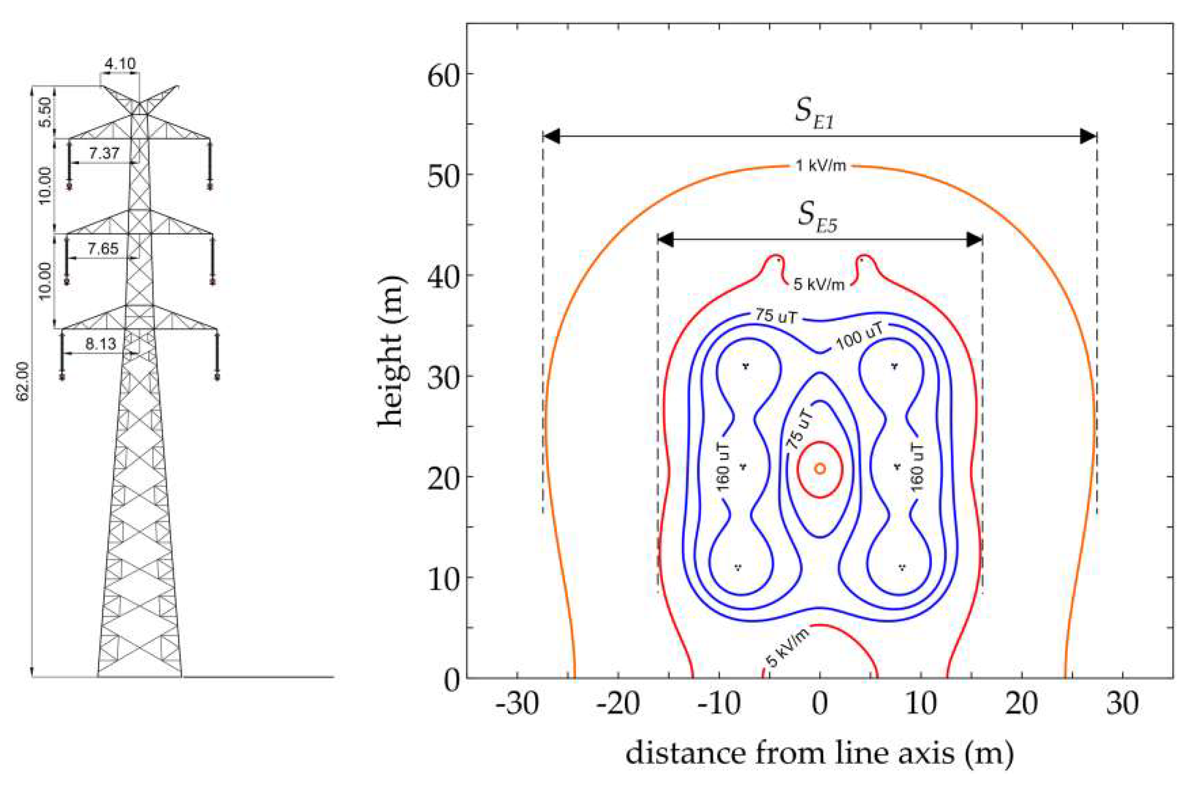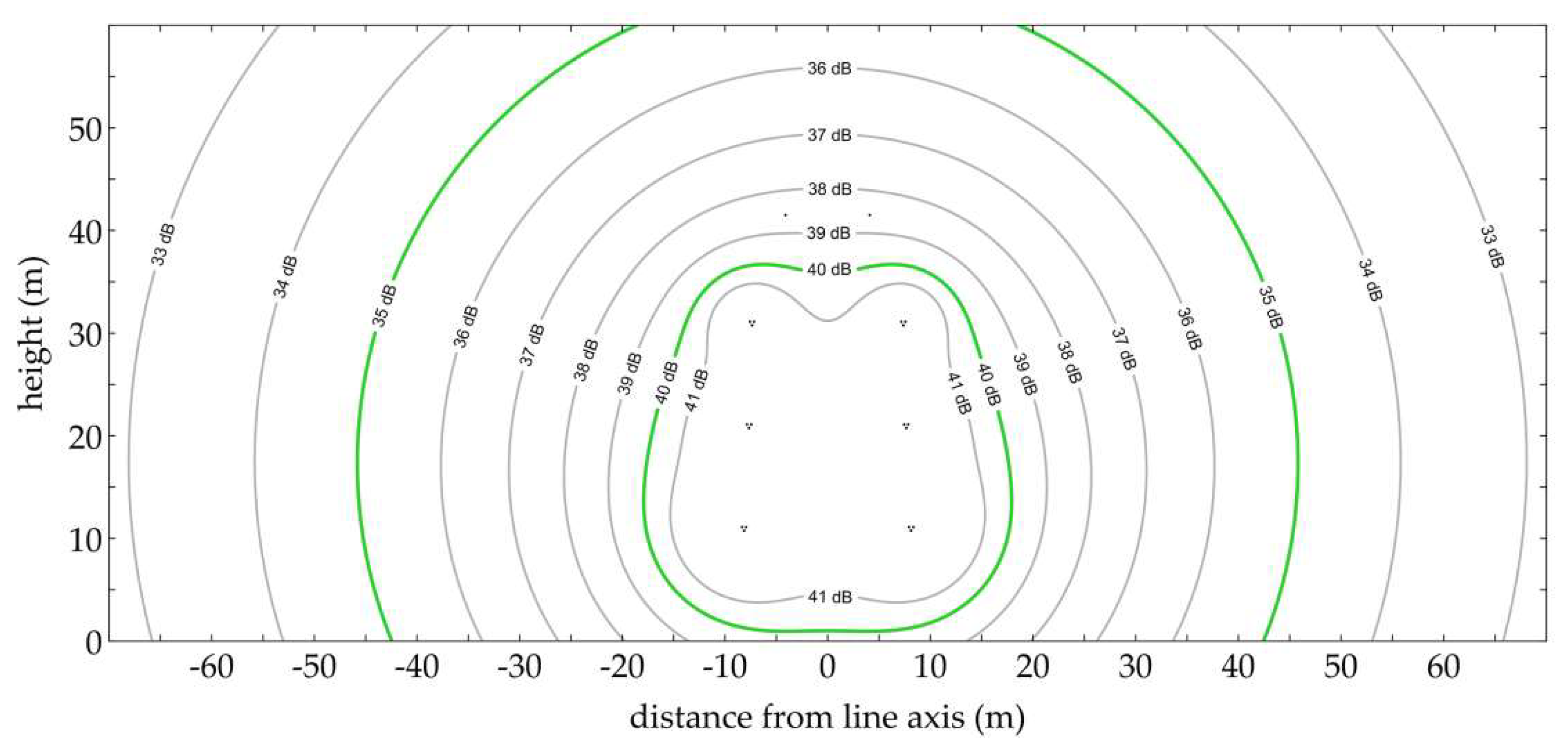Figure 1 presents an example of the electric field and magnetic field in the cross-section of a 400 kV double circuit line. In the example, the assumption of phase voltage symmetry was made, which is complied with in high and extra-high voltage networks. In addition, the load phase symmetry of each circuit was assumed.

These images visualize isolines for reference electric field strengths of 5 kV/m and 1 kV/m, and magnetic field isolines for reference magnetic induction values: 160 µT, 100 µT and 75 µT. These isolines were determined for the highest operating voltage of a 420 kV line, the highest power line current-carrying capacity of the line of 2500 A and the shortest distance of the phase wires from the ground of 11.0 m. The reference values of magnetic induction B = 75 ÷ 160 µT are contained in the space where the electric field strength E > 5 kV/m, as shown in Figure 1. For this reason, the width of the electromagnetic influence zone of a power line is determined by the electric component of the electromagnetic field-widths S_E5 and S_E1 in Figure 1. This statement is true not only for the images shown here, but can be generalized for other overhead power line structures as well.

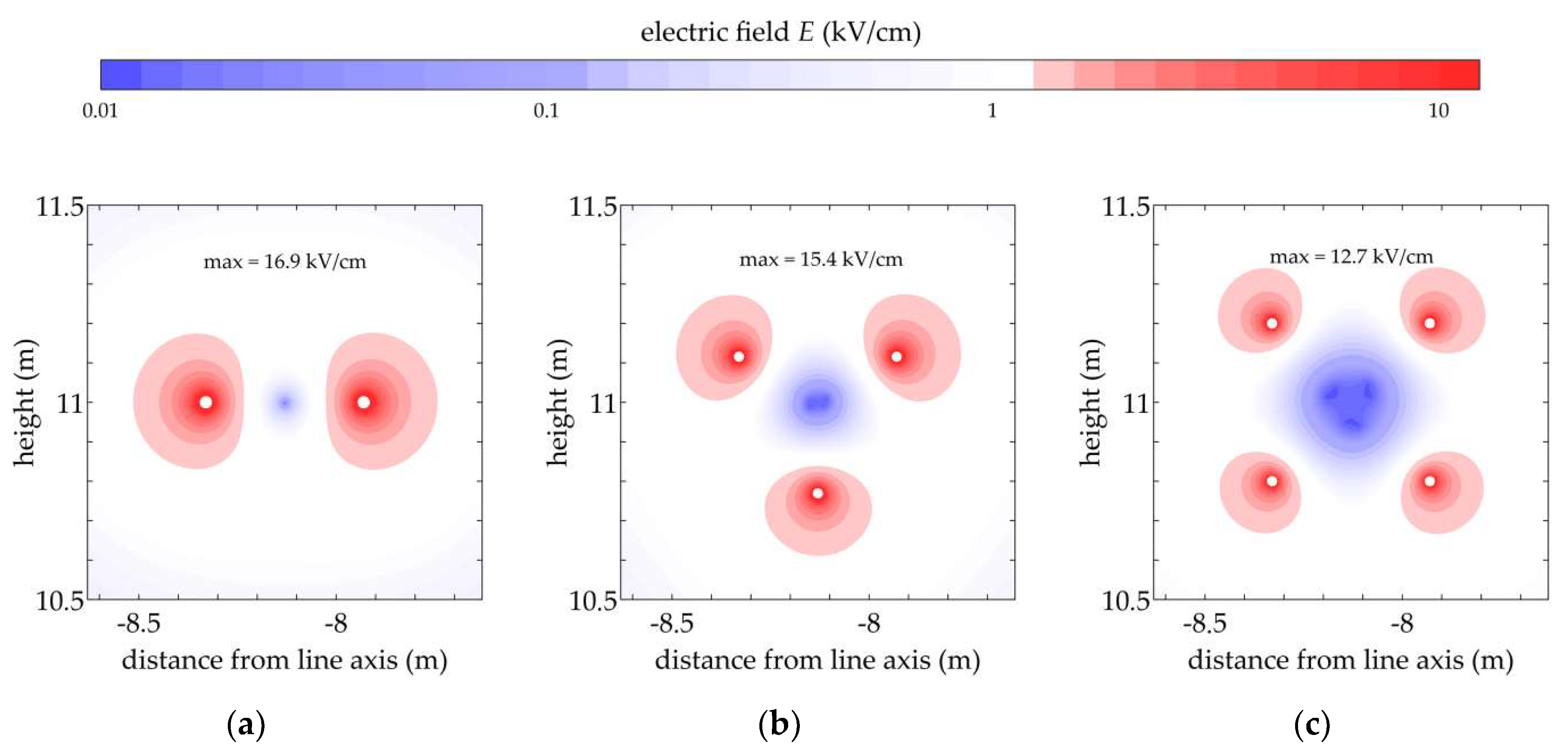
The electric field of overhead power lines is strongly non-uniform, with the highest values occurring at the wire surface. If these values exceed the air ionization onset voltage gradient, the phenomenon of the corona effect will occur in the vicinity of wires. One of the main factors determining corona formation and its intensity is the design of phase wires.

Reduction of the electric field strength on the surface of the phase wires is achieved by using wire conductor bundles (Figure 2). The bundle usually consists of 2 to 4 subconductors.

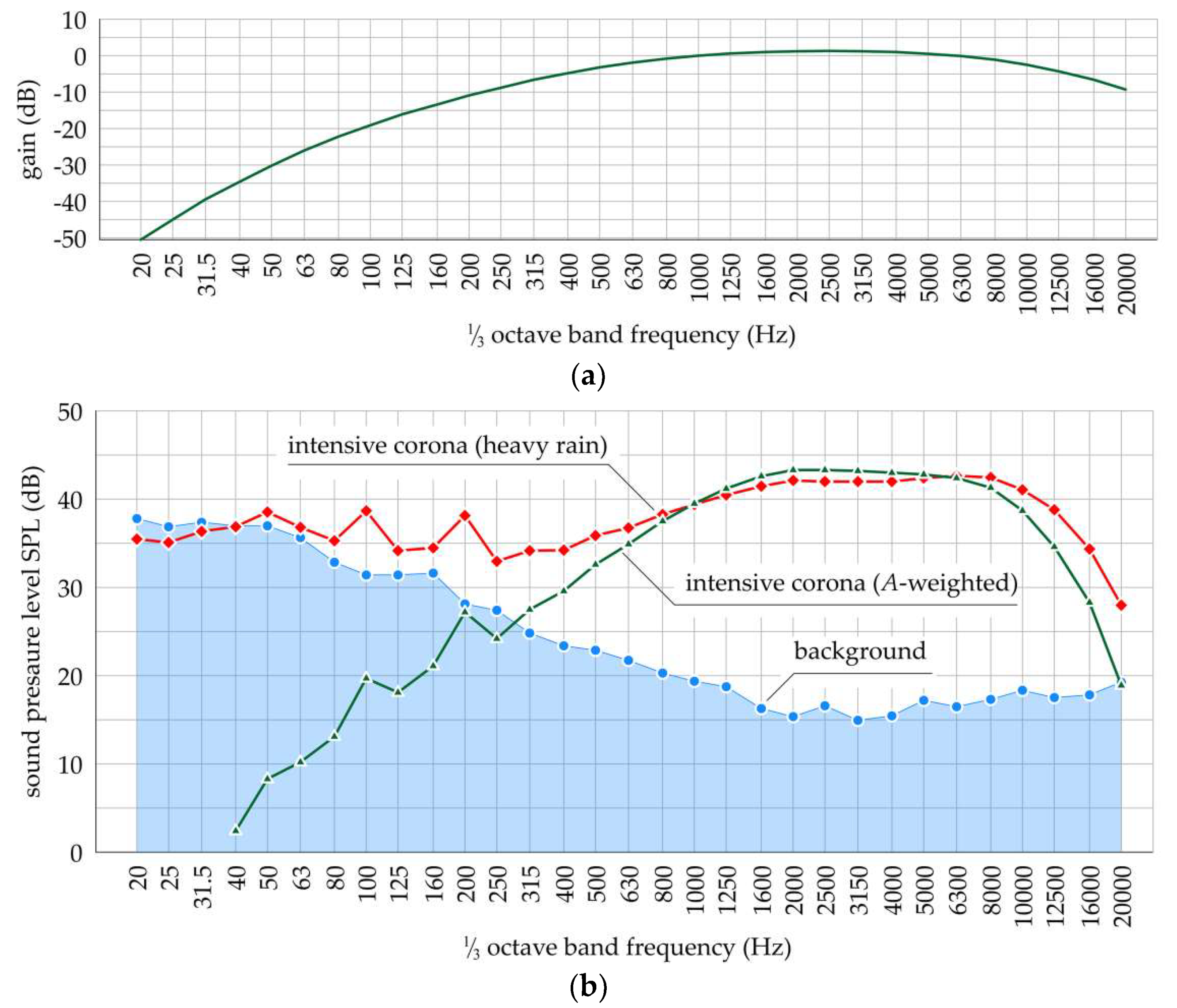
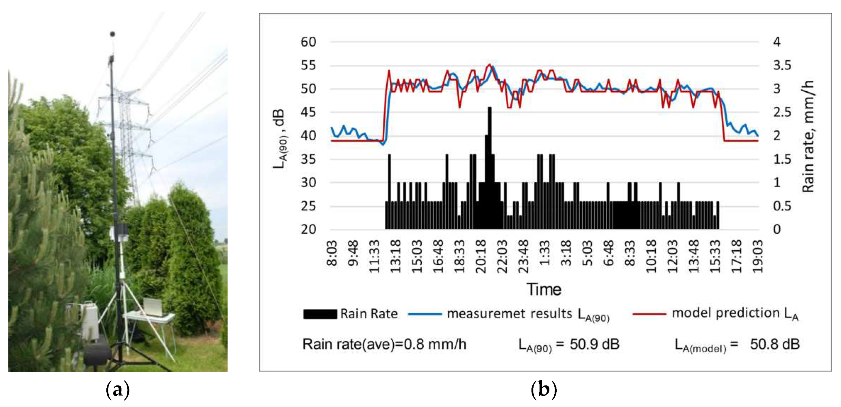
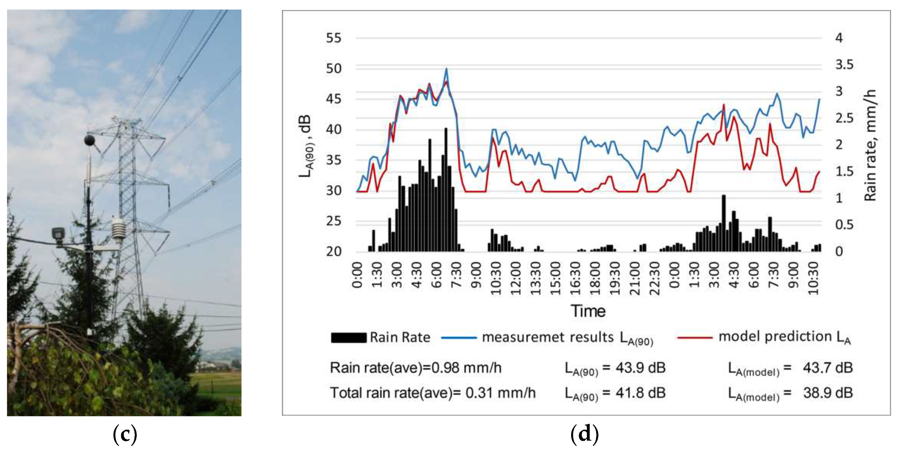
One of the negative corona effects is the audible noise. It significantly differs from the noise generated by other sources, e.g., transportation or industrial sources, because it strongly depends on such random causes as weather conditions or the surface condition of the line wires. The intensity of corona A-weighted audible noise level (Figure 3) in fair weather at a distance of 30 m from the lateral conductor, is about 30 ÷ 40 dB, while on rainy and humid days it may reach up to 55 dB.

International documents [5,6] on the negative environmental impact of noise do not mention power lines as a source. Therefore, general criteria specified in document [7] have been adopted for assessing the environmental effect of noise generated by power lines. In practice, the following impact assessment indicators are used: general indicator of annoyance day-evening-night L_den and detailed indicator of noise annoyance (sleep disturbances) at night L_night. The values of these indicators have been determined 4 m above the ground level.

Document [6] provides recommendations for the highest values of these indicators, and which, depending on the source of noise, are: L_den from 54 dB to 45 dB and L_night from 45 dB to 40 dB. Similar recommendations are included in document [5], in which L_Aeq of 50 ÷ 55 dB during the day, and 5 ÷ 10 dB lower values for the night were assumed as annoying noise values. It should be noted, however, that predicting power line noise and relating the obtained values to the quoted limits is often problematic due to the strong impact of weather conditions on the level of generated noise [8,9].

Authors of this paper study the impact of power line design parameters determining the spatial arrangement of its wires on the width of electric field impact zones S_E5 and S_E1. It should be highlighted the originality of the authors’ research based on the complementary consideration of the electric field and the acoustic emission in the vicinity of the line. Such an approach has not been presented in the subject literature till now. In addition, it should be noted that the analysis was performed using developed programs, and experimentally verified authors models presented in Section 2. These models was used to determine the electric field in the vicinity of the line and on the conductor surfaces, as well as the noise generated by the line. The objects and scope of the study and the construction parameters of single and double circuit lines are described and specified in Section 3. The range of possible changes in the values, resulting from the applied standards and technical feasibility, was determined for these parameters. Section 4 presents the results of investigations of impact of the considered parameters on the widths of zones S_E5 and S_E1 of selected single and double circuit 400 kV lines, as well as the impact on noise levels L_A5 and L_A1 at the border of zones S_E5 and S_E1. The results presented in the article can be used as a basis for selecting the best design solution for the line in terms of minimizing the negative environmental impact. They also suggest possible directions of design changes for lines of other voltages. The results of the analysis presented in the article have allowed us to identify the crucial construction parameters of the line, which is important for the width of the electric field exposure zones. The research has shown that in some cases, it is possible to reduce the width of the zones by up to 50%.

2. Models for the Analysis of Electric Field and Noise Emission of High-Voltage Power Lines

2.1. Electric Field Model

The space in the vicinity of high voltage overhead power lines is the electromagnetic field area. At the network frequency f = 50 Hz, the electric component of this field can be considered independently of the magnetic one. Another simplification is the application of the electrostatic laws to the analysis of the electric field [10]. In general, the basis for calculations are the equations relating the electric field strength E with the electric charges Q accumulated on the elements of the considered system and with their spatial distribution. When writing these equations for the electric field in the vicinity of overhead power lines, the charge simulation method is of particular importance [11,12,13,14,15]. In this method, the actual distribution of charges on the wire surfaces with known potential values are replaced by a set of fictitious charges, so that the electric field induced by these charges is identical with the real one. The simulation charges are assumed to be the geometrically simplest elements, including, but not limited to, line charges, uniformly distributed along a straight line section. Besides the simulated charge method, the finite element method is also used to calculate the field distribution around overhead lines [12,16].

Line models for electric field calculations can be created in both 2-D and 3-D spaces [17]. Figure 4 shows how the wires of an example span (Figure 4a) and the support structure of a double circuit 400 kV line (Figure 4b) are modelled by authors in a 3-D space.

The presented line is equipped with six phase wires in the form of three-conductor bundles (18 conductors in total) and two earth wires. The shape of the catenary curve of each of the wires of the line was approximated by 13 rectilinear sections. The supporting structure was approximated by a set of 352 sections representing profiles making up the lattice tower body. The potentials of sections approximating the phase wires are equal to the phase voltages of the line whereas the potentials of sections approximating earth wires and the support structure are equal to zero.

The calculations are performed with the mirror image method and the potential superposition principle. It was assumed that the earth is a perfectly conducting smooth surface, however, in the literature there are also presented models for the complex terrains under power lines [18]. Based on the above assumptions the following equations can be written for a set of n charges distributed uniformly on the approximating sections (Figure 4):

$$v_i(t)=\sqrt{2}{U}_i\sin \left(2\mathsf{\pi }ft+{\mathsf{\phi }}_i\right)={\displaystyle \sum _{j=1}^n\left({\mathsf{\alpha }}_{ij}-{\mathsf{\beta }}_{ij}\right)}{q}_j\left(t\right),i=1,\dots ,n,$$

(1)

where: v_i(t)—instantaneous potential of the i-th approximating section, U_i—rms value of phase voltage of the i-th approximating section, f—voltage frequency, φ_i—voltage phase, q_j(t)—charge of the j-th approximating section, α_ij—potential coefficient between the i-th and j-th sections, β_ij—potential coefficient between the i-th section and the mirror image of the j-th section.

In Equation (1), the potentials v_i(t) of the approximating sections are known, whereas the potential coefficients α_ij and β_ij are calculated from the geometry of these sections in the assumed coordinate system based on the following relations:

$${\mathsf{\alpha }}_{ij}\mathrm{or}{\mathsf{\beta }}_{ij}=\frac{1}{4\mathsf{\pi }{\mathsf{\epsilon }}_0{l}_i{l}_j}\underset{l_i}{\int }\underset{l_j}{\int }\frac{d{l}_i·d{l}_j}{r}\mathrm{,}$$

(2)

where: r—distance between elements dl_i and dl_j of wires which are l_i and l_j long. Unknown charges q(t) are determined by solving Equation (1). Charges q_i(t)—linear combinations of harmonic functions with the same frequency ω, are harmonic functions defined as:

$$q_i\left(t\right)=Q_i\sin \left(\mathsf{\omega }t+{\mathsf{\Theta }}_i\right),i=1,\dots ,n,$$

(3)

Electric field potential v_B at point B(x,y,z) in the vicinity of a power line can be determined based on section charges (3) and potential superposition principle:

$$v_B(x,y,z,t)={\displaystyle \sum _{i=1}^n\left[{\mathsf{\alpha }}_{Bi}\left(x,y,z\right)-{\mathsf{\beta }}_{Bi}\left(x,y,z\right)\right]\cdot q_i\left(t\right)},$$

(4)

where α_Bi (β_Bi) is a potential coefficient between point B and the i-th section (mirror image of the section). This coefficient directly stems from Equation (9):

$${\mathsf{\alpha }}_{ij}({\mathsf{\beta }}_{ij})=\frac{1}{4\mathsf{\pi }{\mathsf{\epsilon }}_0{l}_i}\underset{l_i}{\int }\frac{d{l}_i}{r}\mathrm{,}$$

(5)

and r is a distance between element dl_i of the i-th wire with length l_i, and point B.

The vector of electric field strength at point B is a potential gradient (4):

$$E=-\mathrm{grad}{v}_B(x,y,z,t),$$

(6)

The following value at point B is assumed while assessing the environmental electric field impact:

$$E_B\left(x,y,z\right)=\frac{\underset{t}{\max }\left\{E\left(x,y,z,t\right)\right\}}{\sqrt{2}},$$

(7)

Based on the above assumptions and Equations (1)–(7), an appropriate numerical calculation agorithms were developed, implemented in the Matlab software, and used for the research presented in this paper.

2.2. Corona-Generated Audible Noise Model

The spectrum of the corona noise signal is a broadband noise spectrum with a random content of tonal components, i.e., higher harmonics of doubled power frequency.

The main energy of the spectrum is contained in the noise part. This is more apparent when the noise signal is passed through a filter with a standardized A (A-weighted) frequency curve [19] (Figure 5a), whose highest values are found in the frequency range from 2 kHz to 4 kHz, corresponding to the noise part of the corona audible noise signal spectrum. The A-weighted noise level corresponds to a loudness level of 40 phonons, and the A-weighted sound level (L_A) is accepted as the best approximation of the human auditory experience up to 70 dB and is a commonly used indicator for assessing noise annoyance. Figure 5b shows a typical unweighted and A-weighted noise signal spectrum from an intense corona in rainy conditions, as well as the ambient noise spectrum during night hours.

In view of the above characteristics of the noise signal spectrum, the existing corona audible noise models refer to an A-weighted level dominated by the noise component, while the tonal components (if present) can be taken into account when determining the rating levels, e.g., by adding the adjustment level to L_Aeq [20,21].

The general form of the noise model incorporates factors affecting the generated sound power level, as well as the distance from the observation point. For a power transmission line, the general model assumes the following form:

$$L_A=k_1\cdot f_1\left(E,E_0\right)+k_2\cdot f_2\left(n\right)+k_3\cdot f_3\left(r\right)+k_4\cdot f_4\left(l\right)+L_0,$$

(8)

where: L_A—predicted A-weighted SPL (dB) at a distance l, E—maximal electric field strength (kV/cm) on the wire surface, E₀—electric field strength (kV/cm) on the wire surface, above which corona takes place, n—number of conductors in the bundle, r—radius (cm) of bundle component wire, l—distance (m) between observation point B and the wire, L₀—noise reference level (dB).

The above form has been adopted to almost all known line acoustic noise models, although they differ in the values of coefficients and sometimes in the forms of particular functions [22].

To determine the level of audible noise generated by extra-high voltage power lines, it is necessary to know the highest values of electric field strength E on the surface of the wires [23,24,25]. These values are determined using the electric field model presented in Section 2.1. For this purpose, K points are selected on the surface of each of the wires and are uniformly distributed around their perimeter, m (e.g., K = 360). At these points the electric field strength is calculated. The highest strength value is determined for the surface of a given wire. In the case of a bundle component wire, the averaged maximum values on the surfaces of the component conductors is taken when determining the sound pressure level.

Electric field strength E₀ (kV/cm), above which the corona effect takes place, is determined by Peek’s empirical formula [25]:

$$E_0=21.2\mathsf{\delta }{m}_1{m}_2\left(1+\frac{0.301}{\sqrt{\mathsf{\delta }r}}\right),$$

(9)

where: δ—relative density of air, m₁—coefficient depending on the condition of the wire and atmospheric conditions (m₁ = 1—for a smooth and dry surface; m₁ = 0.6÷0.8—for a wet surface; m₁ = 0.3 ÷ 0.6—water drops, icicles or major impurities on the surface; m₁ = 0.25—heavy rain), m₂—coefficient accounting for weather conditions equal to 0.8 for rain, r—wire radius (cm).

Based on own studies of a 400 kV line, noise models were developed for establishing sound pressure levels L_Aw(r) and L_Aw(nr) during rain and rain-free conditions, respectively. The general form of these models assumes the following form:

$$L_{Aw\left(r\right)}=10\log \left\{E^{8.5}\left[1-\exp {\left(-0.11{\mathsf{\delta }}_r{\left(E-E_0\right)}^{4/3}\right)}^{1.8}\right]\right\},$$

(10)

$$L_{Aw\left(nr\right)}=10\log \left\{E^{8.5}\left[1-\exp {\left(-0.04/m_s{\left(E-E_0\right)}^{4/3}\right)}^{3.7}\right]\right\},$$

(11)

where: δ_r—rain fall (mm/h), m_s—coefficient depending on the wire condition (m_s ∈ <0.4; 1.0>, m_s = 1—smooth and undamaged wire, m_s = 0.4—soiled wire and/or with a damaged surface.

The total noise emission level L_Ai from the i-th wire of the line is expressed with the formula:

$$L_{Ai\left(r\right)}=L_{Aw\left(r\right)}+\Delta L_{ns}+\Delta L_r+\Delta l-L_0,$$

(12)

$$L_{Ai\left(nr\right)}=L_{Aw\left(nr\right)}+\Delta L_{ns}+\Delta L_r+\Delta l-L_0,$$

(13)

where: L₀—reference level of 63 dB,

$$\Delta L_{ns}=10\log \left(n\right),$$

(14)

$$\Delta L_r=45\log \left(r\right),$$

(15)

$$\Delta l=-10\log \left(l\right),$$

(16)

The summary noise emission level L_A from k phase wires is calculated with the relation:

$$L_A=10\log {\displaystyle \sum _{i=1}^k{10}^{0.1L_{Ai}}},$$

(17)

Based on the above assumptions and Equations (8)–(17), appropriate numerical calculation algorithms were developed, implemented in the Matlab software and used for the research presented in this paper.

2.3. Experimental Validation of Models

In order to verify the electric field model presented in Section 2.1, measurements were performed under a double circuit 220 kV line shown in Figure 6a. They showed a good congruence of measured and calculated electric field strength values. This is confirmed by Figure 6b. It shows a comparison of the measured and calculated distribution in the cross-section of the line at a 2 m height. The conducted research proved the validity of the assumptions made and also confirmed that this model can be used in further analyses on the reduction of electric field impact zones of overhead power lines.

To verify the power line corona audible noise model presented in Section 2.2, measurements were conducted in the vicinity of a double circuit 400 kV line with N = 2 bundle wires (Figure 7a) and in the vicinity of a double circuit 400 kV line with N = 3 bundle wires (Figure 7c). Figure 7b,d compares the measured results during rain with the results obtained from model calculations.

A monitoring station SVAN210 with a GRAS microphone 40 AE was used for the verification of measurements. Meteorological measurements were performed with a WatchDog 2900 station and Vaisala Airmar Station PB100. Acoustic signals at both stations were recorded in 1/3 octave bands ranging from 10 Hz to 20 kHz, with a time resolution of 10 s. Measurements were conducted over a period of approximately one and a half days (35 h), and the measurement values were averaged with a 15-min resolution. The comparative analyses of the measured and calculated signal were made with level L_A(90), i.e., A-weighted statistical (percentiles) L₉₀ level (the level exceeded for 90% of the time).

The verification of the model calculations lied in using actual (measured) values of rainfall intensity and carrying out model calculations for them. The obtained results are given in Figure 7b,d. The output of calculations was performed according to the proposed corona audible noise model, which coincides with the measured results in the rainfall conditions.

In analyzed cases, the average difference in the whole measurement window (during rain) is 0.1 dB (Figure 7b) and 0.2 dB (Figure 7d). For the line with N = 2 bundle, the measured value of L_A(90) level during rain (from 12:00 to 15:30 the next day) is 50.9 dB and the calculated value during this time interval L_A(model) = 50.8 dB. For the line with N = 3 bundle, the measured value of L_A(90) level during rainfall is 43.9 dB, and the calculated value during this time interval L_A(model) = 43.7 dB. For the entire measurement interval shown in Figure 7d, which also includes rain intervals, the measured L_A(90) level is 41.8 dB and the model calculated value L_A(model) for this time equals to 38.9 dB.

The values in individual 15-min windows vary much more in Figure 7b even 4–5 dB, and the standard deviation of the difference between these levels is 1.95 dB. In general, the calculated results for this case are only slightly different from the measured results, mainly due to the continuous rainfall and the noise associated with it. The measurement window of the line with the N = 3 bundle is characterized by a high variability of rainfall intensity, and consequently variability of the accompanying noise emission (Figure 7d). The average difference over the entire measurement window (with moments of no rain or very little rain) is 1.9 dB. However, in the part of the measurement window between 3:00 and 5:00, when the rainfall was more uniform, the results of model calculations (L_A(model) = 45.4 dB) practically do not differ from the measured results (L_A(90) = 45.3 dB). Furthermore, it should be noted that during the short intervals between rainfall occurrences, the wires stay wet, resulting in higher noise emissions than model calculations would predict. This can be seen in the 7:30 and 1:30 time interval (Figure 7d). The maximum differences between the measured and calculated values in the 15-min windows may exceed 8 dB, with a standard deviation of 2.6 dB. Such a discrepancy of the results mainly stems from the high inertia of the corona effect. This is especially evident in the time between 1:30 and 9:00 the next day (Figure 7d), where the measured results are much higher than the calculated values. This is caused by the fact that the model does not take into account the inertia of the corona effect when rainfall stops. Model calculations in the case of precipitation disappearance are usually performed as for dry wires. In reality, however, the wires are wet for a long period of time and the corona with its accompanying phenomena (though less intense) still takes place. However, the problem of inertia is negligible in the noise prediction practice. The calculations make use of average values or possibly the maximum precipitation value, as the maximum sound generation due to corona occurs during the rain.

3. Subject and Scope of Research

The computational models presented in Section 2 were used for analyzing zone widths S_E5 and S_E1 of the electric field impact of 400 kV lines, and studying noise levels L_A5 and L_A1 at the borders of zones S_E5 and S_E1. The tests were performed for single and double circuit 400 kV power lines, whose symmetrical wire configurations and arrays are shown in Figure 8. The analysis assumes symmetry of the phase voltages.

Structural parameters (

Table 2. Analyzed design parameters of the overhead power line.

Symbol	Parameter Description
xP	outer phase conductor horizontal distance to axis of the single circuit line outer phase conductor horizontal distance to axis of the double circuit line
hP	conductor height at tower
ΔhP	inner phase conductor horizontal distance to outer phase conductor phase-to-phase vertical distance in the double circuit line
xE	earth wire horizontal distance to axis of the double circuit line
ΔhE	earth wire vertical distance to lowest conductor
fP	conductor sag
fE	earth wire sag
N	number of subconductors per bundle
b	subconductor distance within a bundle

), which are significant for the zone widths S_E1 and S_E5, were indicated for the feasibility analysis of electric field impact reduction. The purpose of this study was to determine the effect of changes in these parameters on the possibility of reducing S_E1 and S_E5 zones.

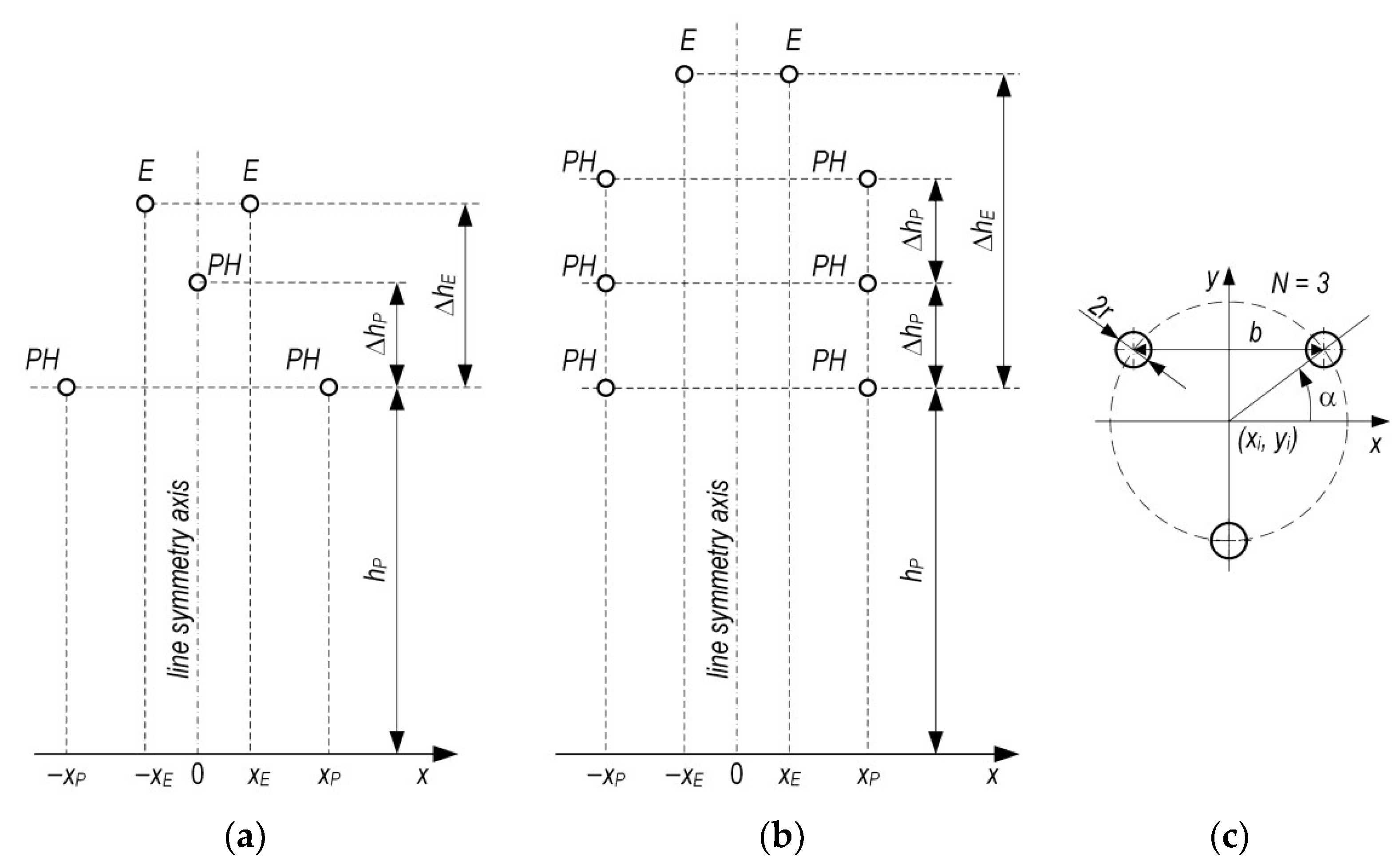
The parameters shown in Table 2 can be classified into three groups. The first group includes parameters x_P, h_P, and h_P, which determine the geometric arrangement of phase wires in the line’s cross-section. Together with parameter f_P they form a system that gives full information about the location of phase wires in a given line’s cross-section. The values of h_P and f_P parameters are closely related to the required distance from the ground. The second group includes parameters x_E and h_E, which together with f_E determine the place of the earth wires. The third group consists of N and b parameters that characterize the structure of the bundled phase conductors (Figure 7c).

The range in which these parameters oscillate results from the normative requirements [26] ensuring safety insulation clearances determined by the rated voltage, overvoltage and environmental conditions. Permissible ranges and typical values of parameters of the 400 kV line are given in

Table 3. Admissible ranges and typical values of analyzed parameters of support structures.

Line Parameter	Single Circuit Lines		Double Circuit Lines
	Range	Typical Example	Range	Typical Example
xP (m)	6 ÷ 12	10.3	4 ÷ 9	8.45
hP (m)	Depends on conductor sag
ΔhP (m)	0 ÷ 2	0	6 ÷ 10	9.2
xE (m)	5 ÷ 12	7.5	0 ÷ 8.5	6.15
ΔhE (m)	6.5 ÷ 15	7	10	10
fP (m)	Depends on conductors design and tension
fE (m)	Depends on conductors design and tension

and

Table 4. Admissible ranges and typical values of analyzed conductor bundle parameters.

Conductor Parameter	Range	Typical Example
N	2 ÷ 4	2 ÷ 3
b (mm)	350 ÷ 500	400

.

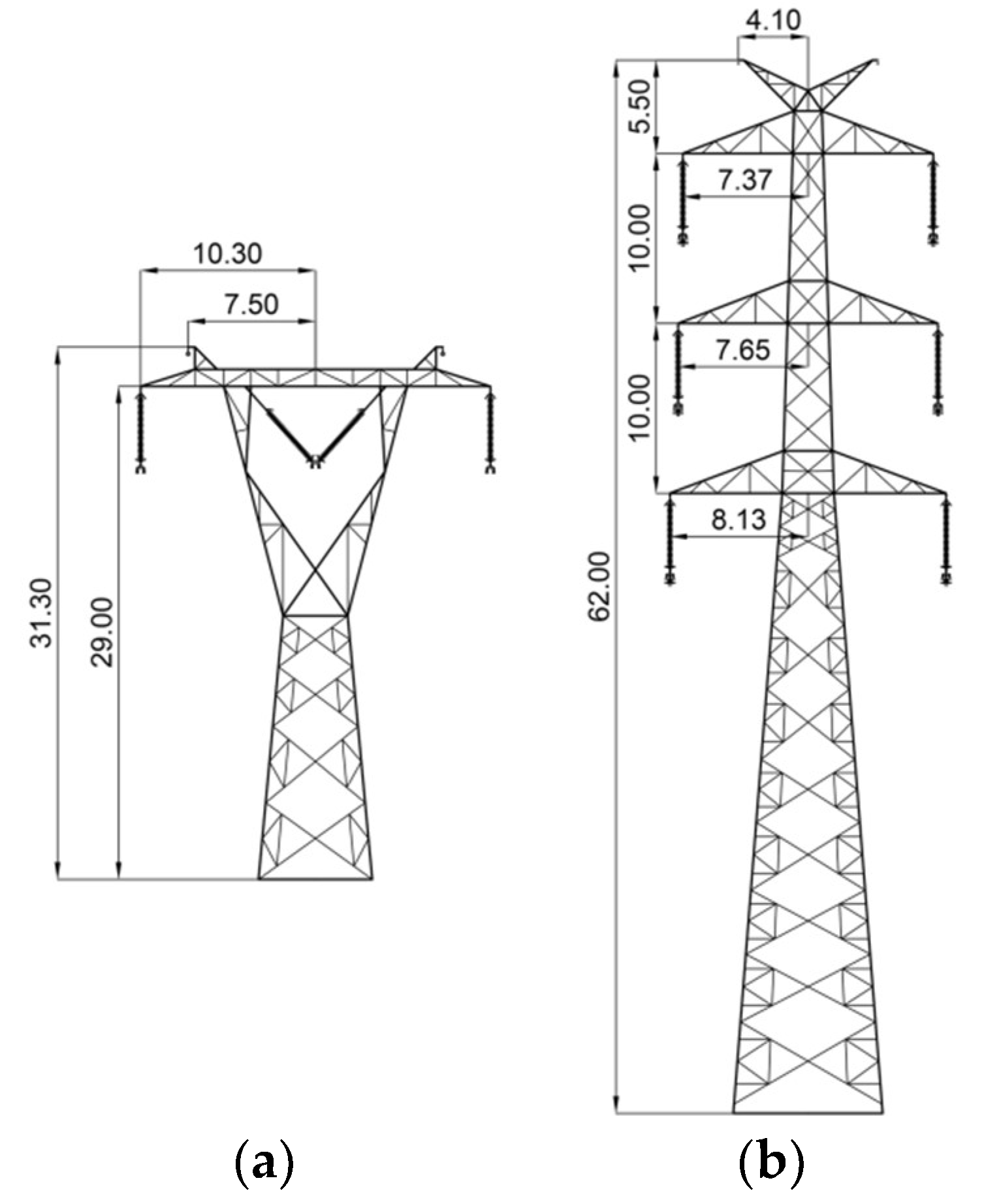
Figure 9 shows the schemes of the single and double circuit 400 kV line towers adopted for the study. The indicated dimensions can be treated as typical for this level of rated voltage.

In the single circuit line (Figure 9a), the phase conductors were assumed to be made as double conductor bundles N = 2, 2r = 31.50 mm, b = 400 mm and form a flat conductor configuration. Whereas in the double circuit line (Figure 9b) an assumption was made that the phase wires are made as triple conductor bundles N = 3, 2r = 26.10 mm, b = 400 mm forming a vertical conductor configuration. The insulator chains are 5.50 m long, except for the central phase chain of the single circuit line, for which the length is 5.25 m. Moreover, span lengths of 450 m, as well as equal phase and earth wire sags f_P = f_E = 13.5 m were also assumed.

4. Analysis of Influence of Line Design Parameters on SE5 and SE1 Zone Widths

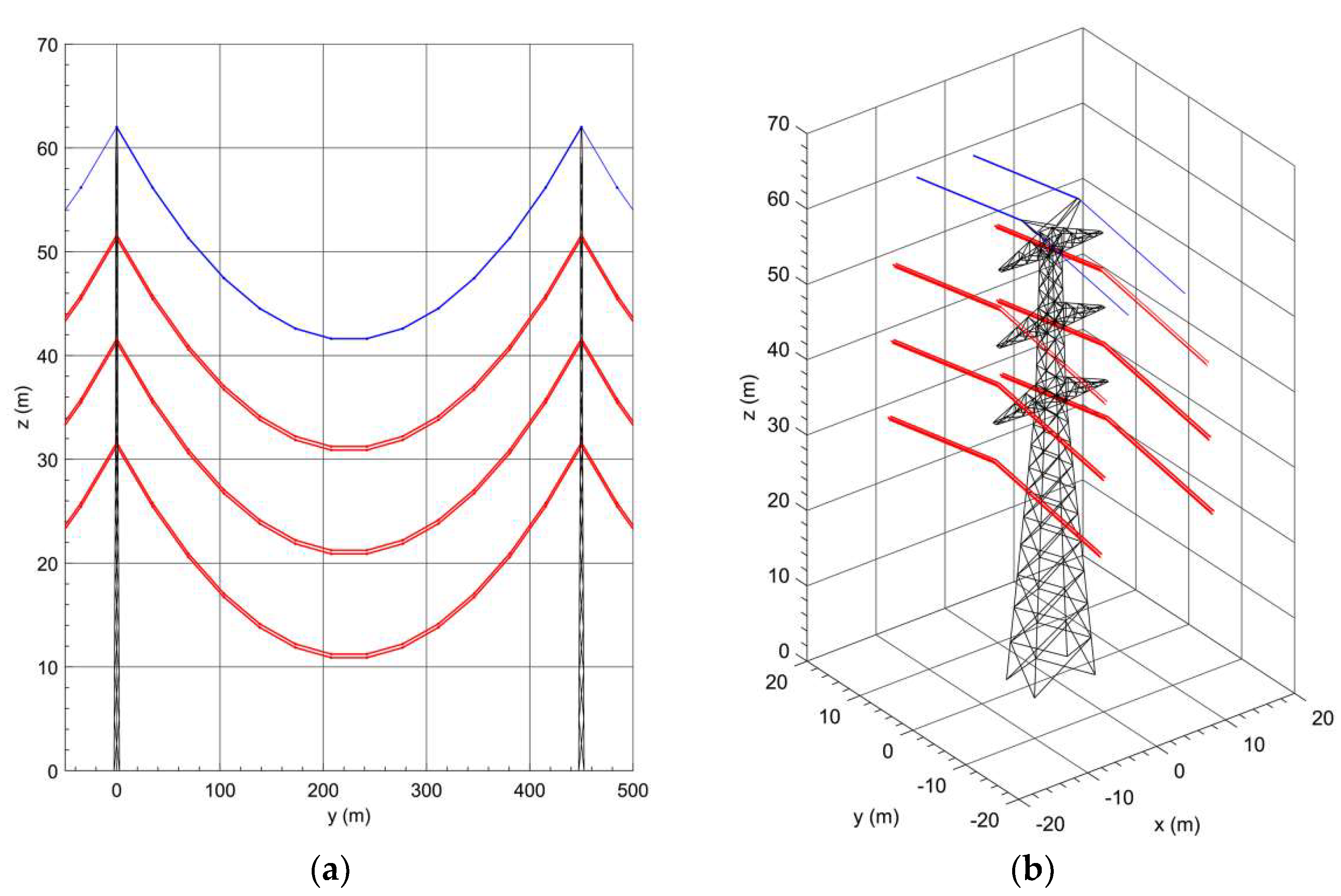
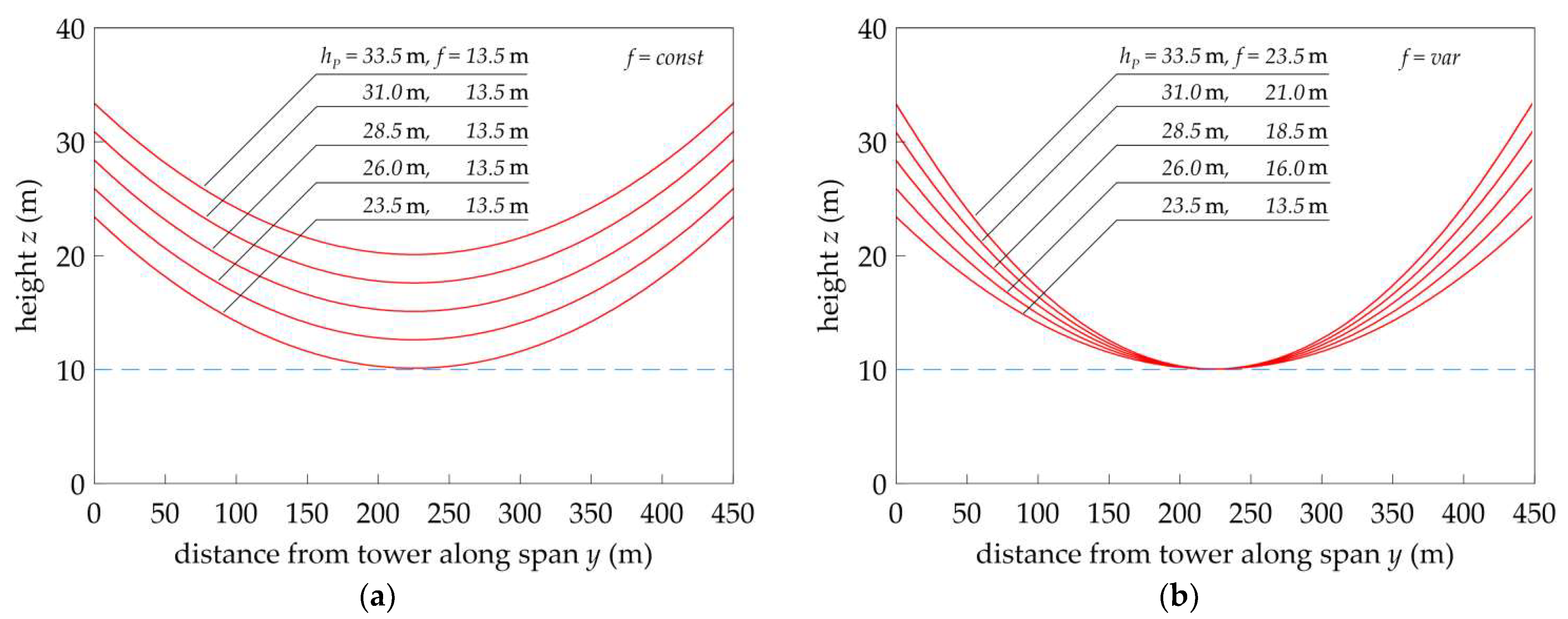
The first step of the analysis lied in checking out whether or not it is possible to reduce the width of the single circuit line impact zone (Figure 9a) by increasing the wire height h_p at tower from 23.5 m to 33.5 m. Figure 10 shows the outer phase conductor profiles for selected heights h_p. The analysis considers both the case of a constant sag f_P = f_E = 13.5 m (Figure 10a) and variable sag f_P = f_E = var situation at a constant minimum conductor-to-ground distance of 10 m (Figure 10b). 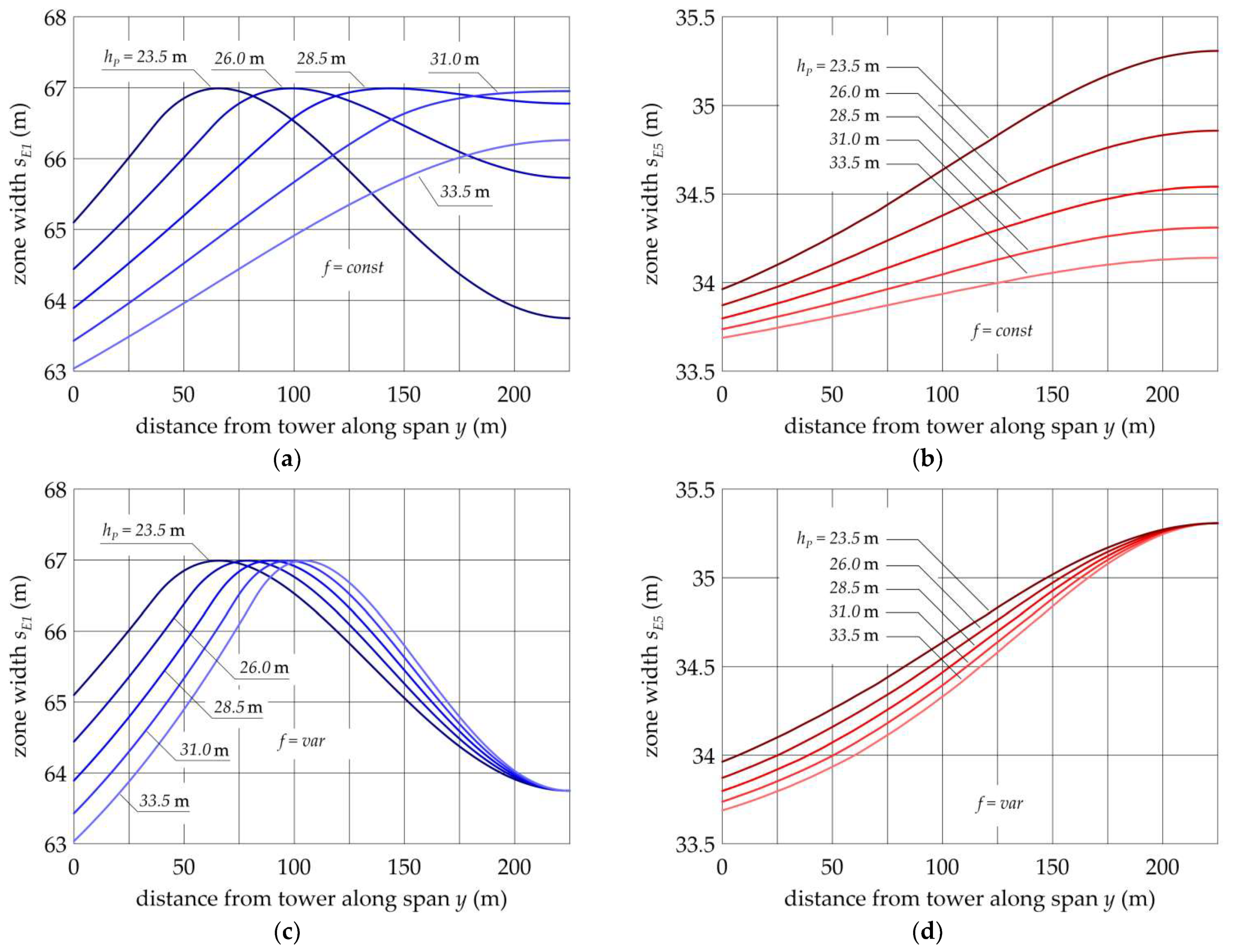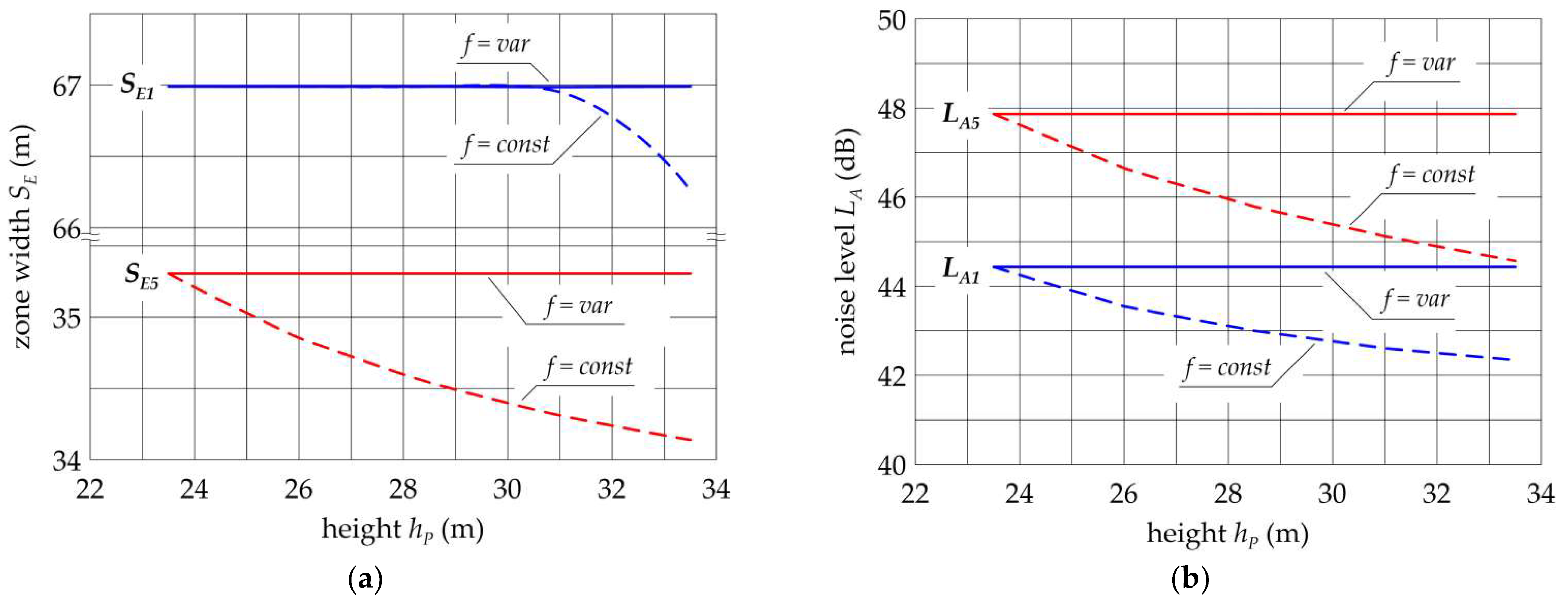Figure 11a,b illustrate the widths of zones S_E5 and S_E1 along the line span for a constant sag case, and Figure 11c,d for a variable sag case. On the other hand, the dependence of zone widths $S_{E5}=\underset{y}{\max }\left[s_{E5}\left(y\right)\right]$ and $S_{E1}=\underset{y}{\max }\left[s_{E1}\left(y\right)\right]$ in a function of conductor height h_p on tower is presented in Figure 12a.

Figure 12a shows that for f = var, the zone widths do not depend on height h_p. For f = const, the zone widths decrease with the increase of height h_p, zone S_E1 is reduced by 0.7 m and zone S_E5 by 1.2 m. It should be noted that the increase of height h_p has a negligible effect on the zone width reduction, but it has a significant effect on the noise level decrease. This has been illustrated in Figure 12b showing a relationship of corona audible noise levels L_A1 and L_A5 at the boundary of S_E1 and S_E5 zones. The noise impact is reduced for f = const. In this case, by increasing the height of conductors by 10 m the noise levels L_A1 and L_A5 are reduced by 2.1 dB and 3.3 dB, respectively.

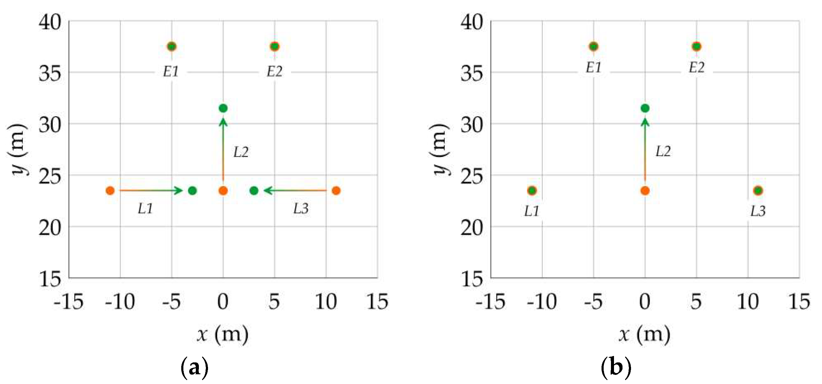
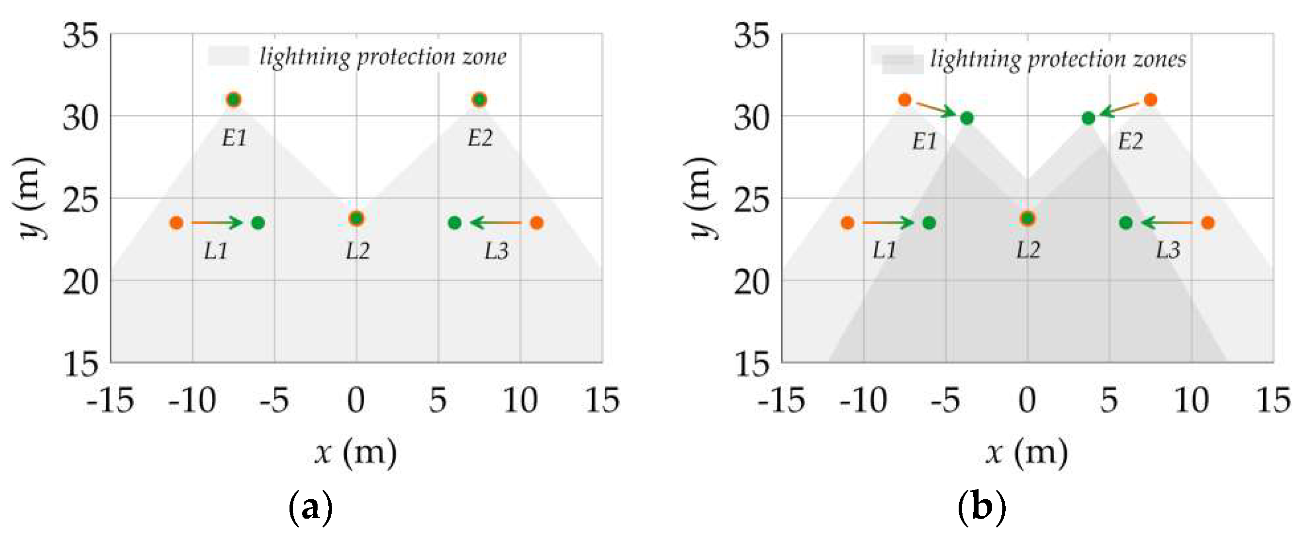
In the next step of the analysis, parameter x_P was examined for different values and the effect it brings about. Two variants shown in Figure 13 were considered.

In the first variant (Figure 13a) an unchanged position (x_E, Δh_E = const) of earth wires is assumed to ensure a continuous lightning protection area. The zone shown in Figure 13a refers to the outermost phase and the inner phase conductor angles of lightning protection of 20° and 45°, respectively. In the second variant (Figure 13b), it is assumed that the decrease of x_P is accompanied by a simultaneous change in the position of earth wires (x_E, Δh_E = var) to ensure constant values of the outermost phase and the inner phase conductor protection.

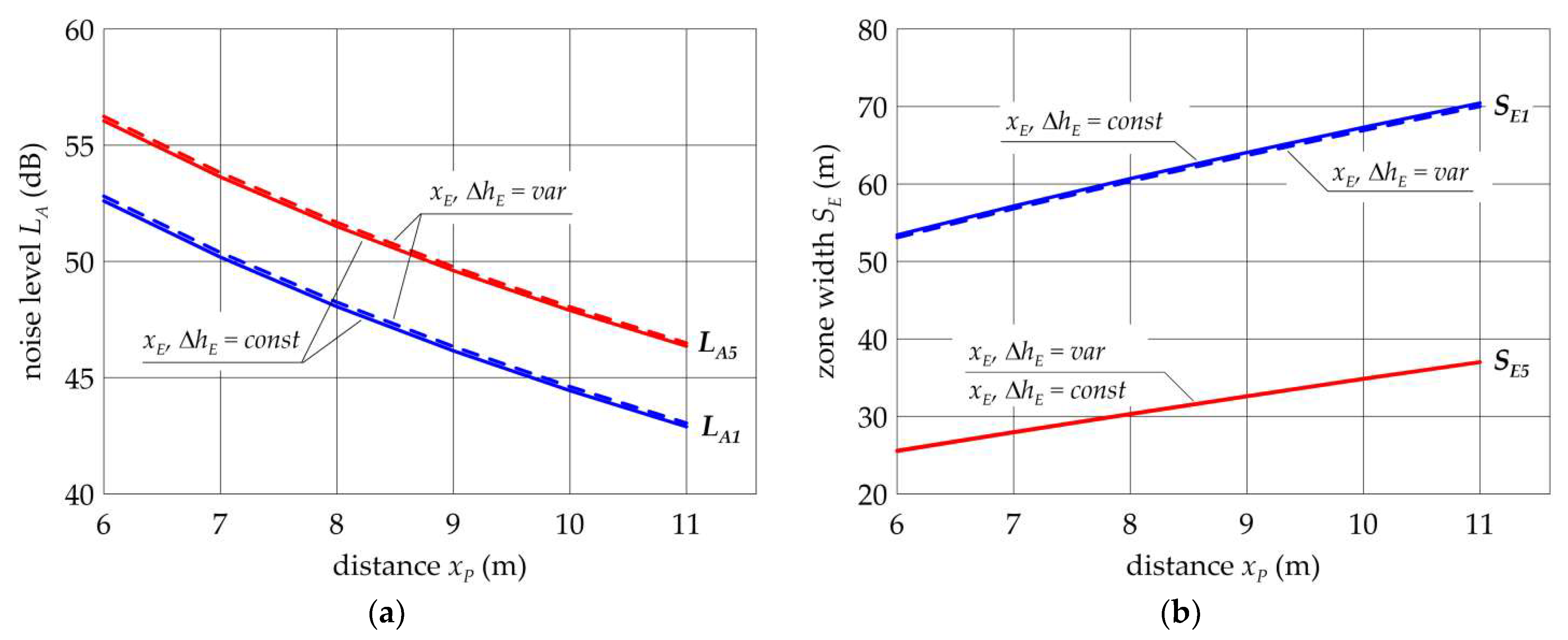
Figure 14a shows the width dependence of zones S_E1 and S_E5 as a function of distance x_P, and Figure 14b visualizes the noise level dependence of L_A1 and L_A5. The variation of x_p between x_P(min) = 6 m and x_P(max) = 11 m was considered. The value of x_P(min) results from normative requirements (e.g., [26]) regarding voltage-dependent clearance distances. On the other hand, the value of x_P(max) is limited by both technical and economic factors. The technical constraints arise from the increase in the tower bending moment with the growth of x_P. This, in turn, results in the higher cost of the tower, and consequently, the need to increase the mechanical strength of its structure and foundations. Another constraint of an economic nature is the increasing width of the right of way.

Figure 14 shows that both zone widths and noise levels are virtually independent of the location of earth wires. With the decreasing distance x_P from 11 m to 6 m zone width S_E1 is narrowed by 17.0 m (24.1%), and zone S_E5 by 11.4 m (30.9%). However, this reduction is accompanied by a significant increase in noise levels L_A1 and L_A5 by 9.8 dB.

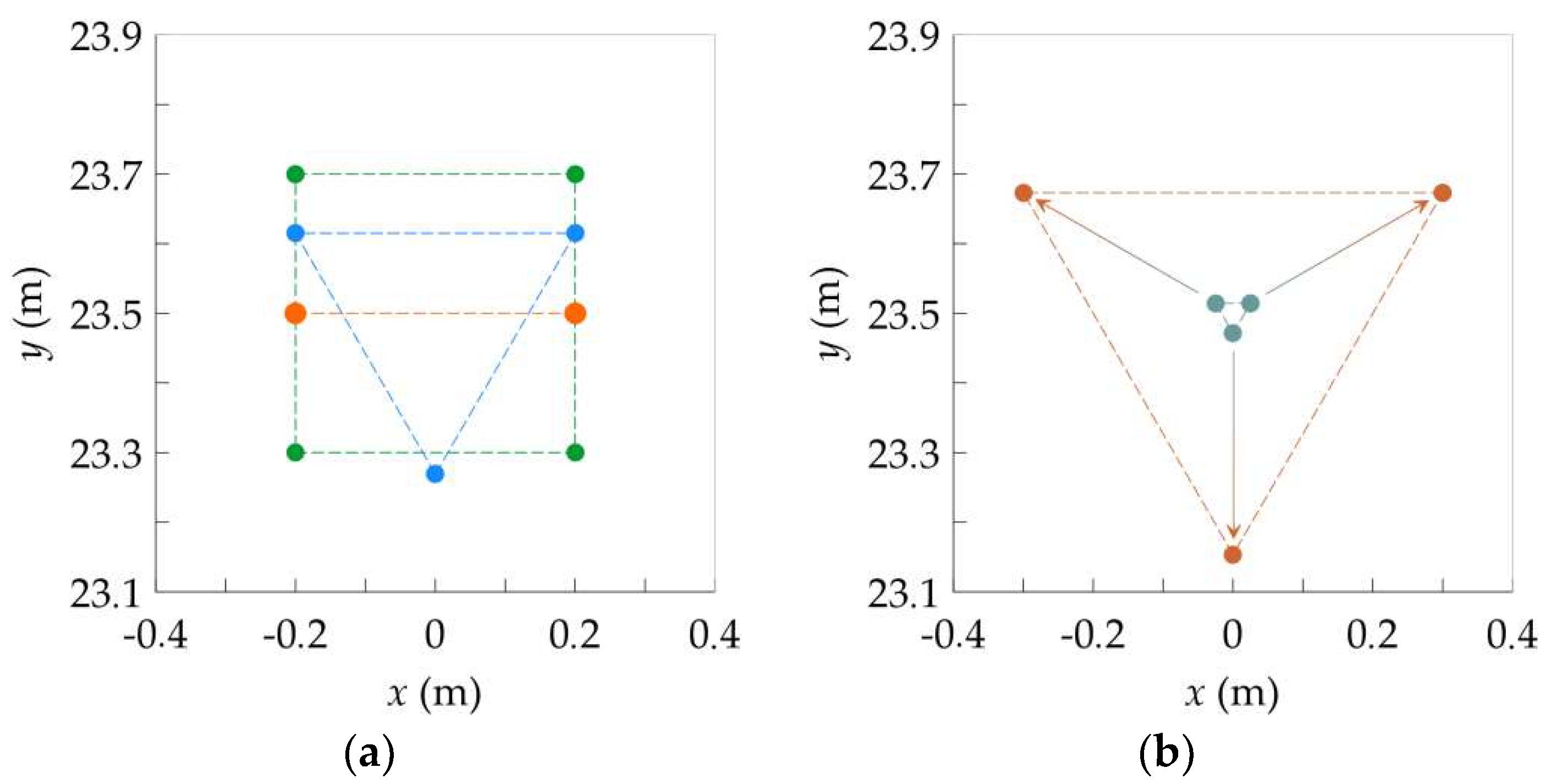
The range of parameter x_P values can be broadened in the analyzed 400 kV line below the lower boundary x_P(min) = 6 m if the phase conductor configuration is changed from flat to triangular. Two variants of this reconfiguration, involving the increase the height of the central phase by Δh_P = 0 ÷ 8 m, are presented in Figure 15. The first variant assumed a simultaneous decrease of parameter x_P from x_P(max) = 11 m to x_P(min) = 3 m (Figure 15a). In the second variant, a constant value of x_P = 11 m is assumed for the outermost phase (Figure 15b).

Increasing the height of the central phase conductor while decreasing the distance of the outermost phase conductors (x_P = var), significantly reduces the width of the electric field impact zones (Figure 16a). In the analyzed 400 kV line, a narrowing of the zone width S_E1 by 31.2 m (44.2%), and zone S_E5 by 18.3 m (49.4%) is achieved. However, this reduction is accompanied by a significant increase in noise levels L_A1 and L_A5 by 10.1 dB and 9.7 dB, respectively (Figure 16b). If the position of the outermost phase conductors remains the same (x_P = var), the change of distance Δh_P does not affect zone widths S_E1 and S_E5, though reduces noise levels L_A1 and L_A5 by 2.8 dB.

The considerations presented so far concentrated on a 400 kV line in which phase conductors consisted of two-sub-conductor bundles with the following parameters (Figure 8c): N = 2, 2r = 31.50 mm, b = 400 mm, α = 0°. The type of the applied bundle conductors affects the electromagnetic and noise impact of the power lines. Further studies of the case shown in Figure 15a were carried out to analyze this influence. Two options were considered: (i) changing number N of sub-conductors in the bundle, (ii) changing distance b between sub-conductors in the bundle.

In the first variant, the tests were carried out for three types of bundled conductors (Figure 17a): (i) N = 2 (2r = 31.50 mm, b = 400 mm, α = 0°), (ii) N = 3 (2r = 26.10 mm, b = 400 mm, α = 30°), N = 4 (2r = 26.10 mm, b = 400 mm, α = 45°). In the second variant, the tests were performed for N = 3 conductors, assuming a variation of distance b from 50 mm to 600 mm (Figure 17b).

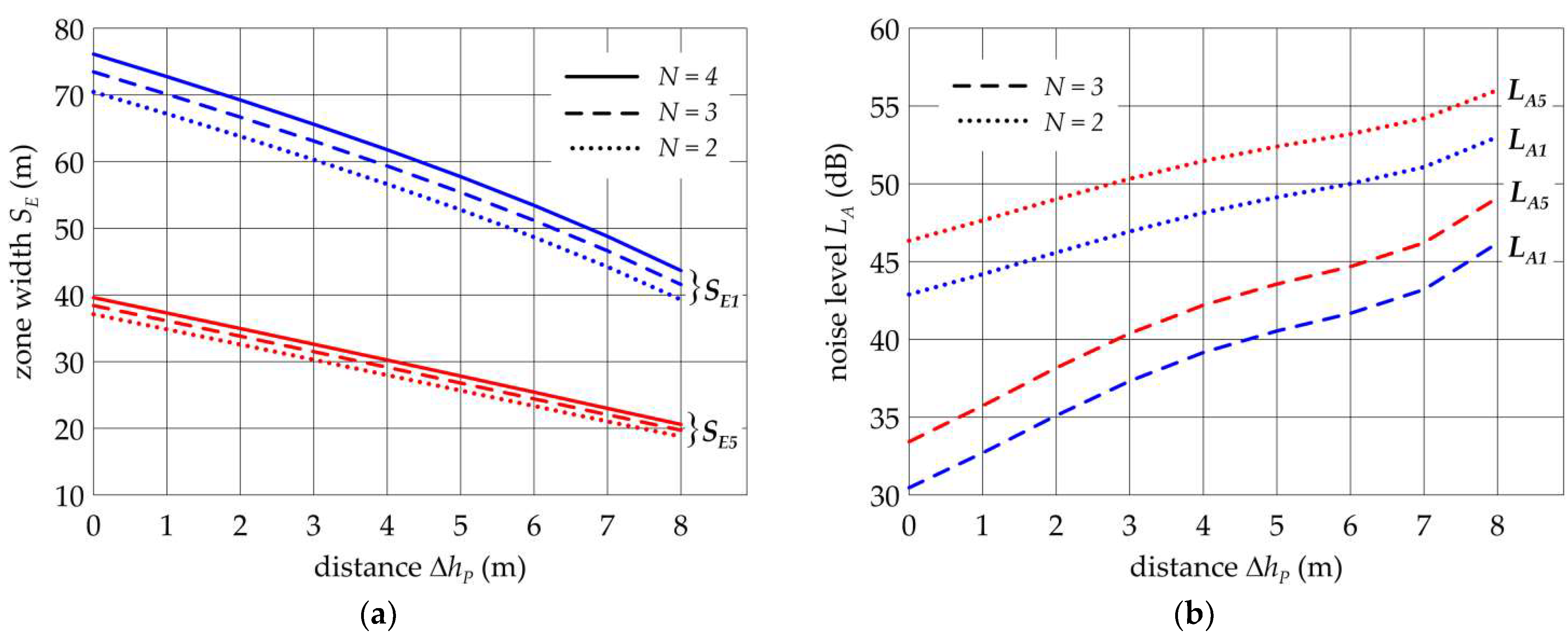
The increasing number of N wires in a bundle results in a broader width of zones S_E1 and S_E5 (Figure 18a). For Δh_p = 0 (flat configuration) the triple bundle (N = 3) increases the zone width S_E1 by 3.0 m (4.3%) and zone S_E5 by 1.3 m (3.5%), as compared to the zone widths of double conductor lines (N = 2). For the quadruple conductor bundle (N = 4), these values are even higher and are 5.7 m (8.1%) and 2.5 m (6.7%), respectively. For Δh_p = 8 m the triple conductor bundle (N = 3) makes zones S_E1 and S_E5 wider by 2.3 m (5.8%) and by 0.9 m (5.0%), respectively. In the case of a quadruple conductor bundle (N = 4), these values are 4.4 m (11.1%) and 1.8 m (9.7%), respectively.

Although the increased number N of conductors in a bundle is associated with an adverse effect of a bigger electromagnetic impact, a significant reduction of noise impacts is achieved (Figure 18b). When a three conductor bundle (N = 3) is used, the noise levels L_A1 and L_A5 decrease by ca. 12.5 dB for Δh_p = 0 m and by about 6.9 dB for about Δh_p = 8 m as compared to a double conductor bundle line (N = 2). In the case of a quadruple conductor bundle line (N = 4), the electric field strength at the wire surface is below the initial corona, and no noise impact is observed.

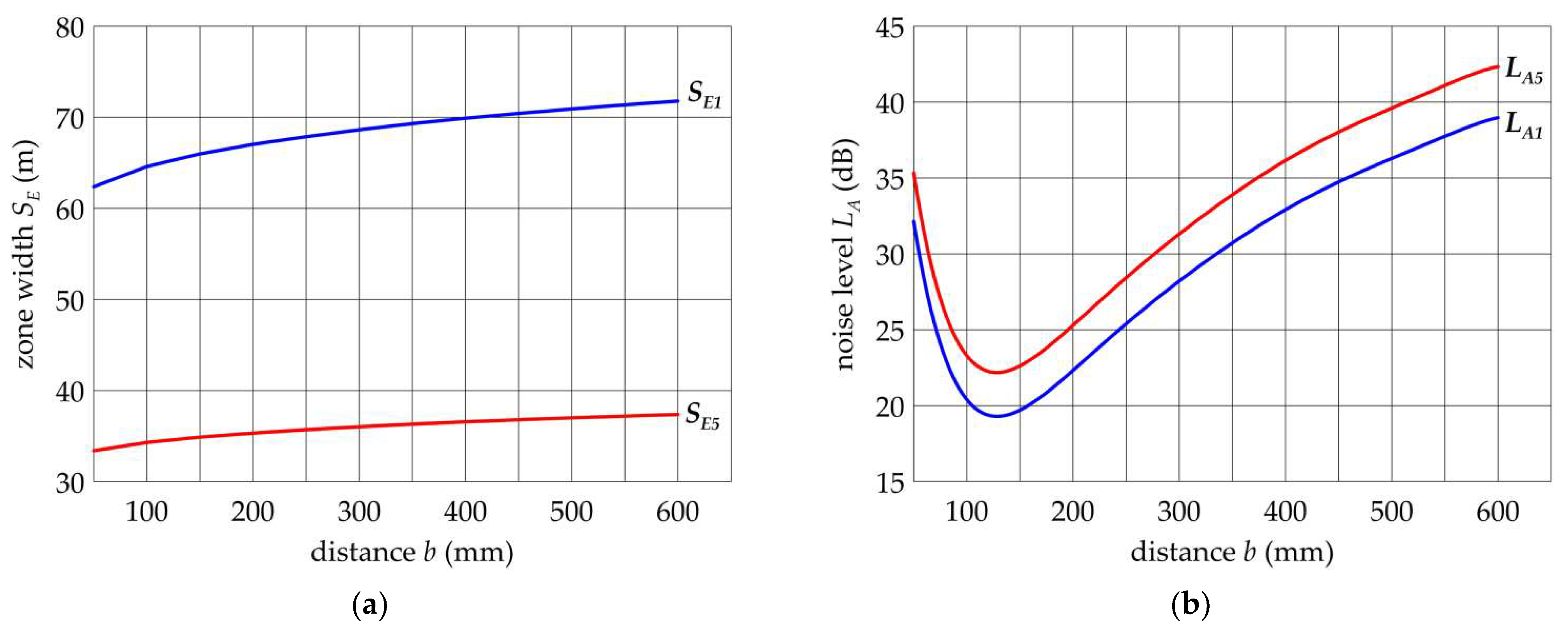
The sub-conductor distance b in the bundle affects zone widths S_E1 and S_E5 (Figure 19a). In the considered range of distance b from 50 to 600 mm the zone width S_E1 increases by 9.4 m (15.1%) and S_E5 by 4.0 m (11.9%). The effect of parameter b on the noise level is complex (Figure 19b). Initially the values of L_A1 and L_A5 decrease with the increase of b and for b ≈ 150 mm reach the lowest values 19.7 dB and 22.7 dB. A further increase of b results in an increase of the noise level values. However, in practice, the problem of choosing the optimum value of distance b is complex. Many other factors influence the choice, primarily the number of sub-conductors, in the bundle climatic conditions and the resulting need to prevent excessive icing as well as the effects of sub-span vibrations between conductor spacers. For these reasons, distance values b are usually equal to 300–500 mm.

Conclusions resulting from the analyses of the single circuit lines are also valid for double circuit lines as far as qualitative aspects are concerned. This applies first of all to the impact of x_p parameter, which in the case of the double circuit lines is the phase conductor horizontal distance to the axis, and the effect of the phase conductors design. Figure 20 shows the range of changes of the phase conductors on a double circuit 400 kV line adopted for the analysis from Figure 9b. A constant location of earth wires was assumed x_E, Δh_E = const and a constant distance Δh_P = const phase conductors. 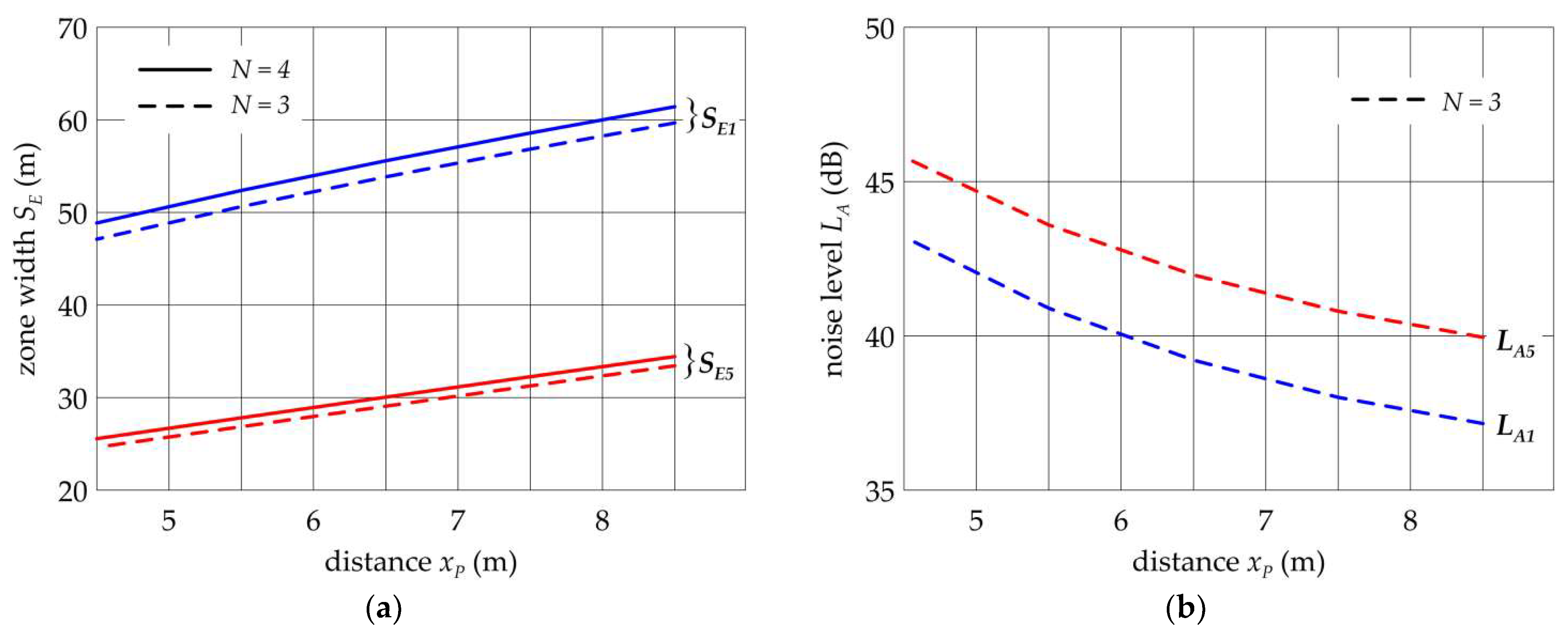Figure 21a shows the zone width relationships of S_E1 and S_E5 in a function of distance x_P, and in Figure 21b noise levels L_A1 and L_A5. Consideration was given to the change of x_p from x_P(min) = 4.5 m to x_P(max) = 8.5 m. As in a single circuit line, the value of x_P(min) results from normative requirements, and the value of x_P(max) is limited by technical and economic constraints.

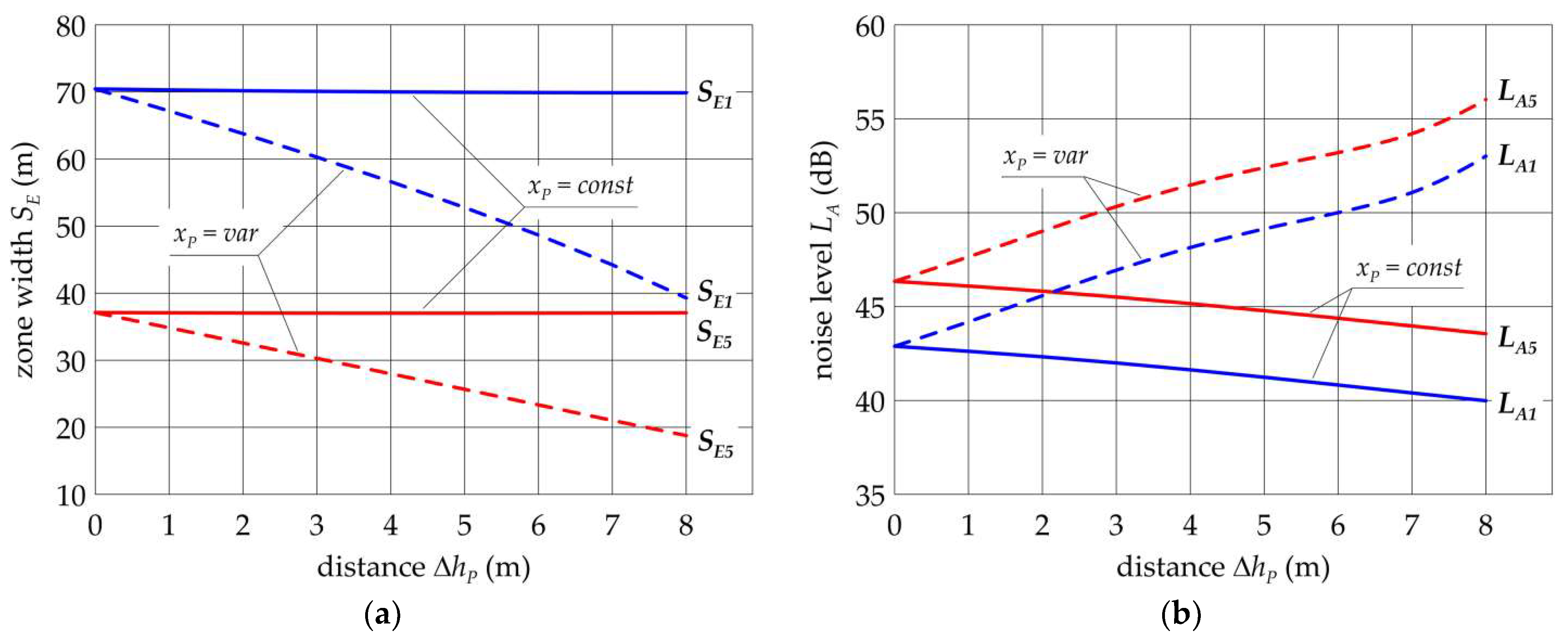
Figure 21 shows that regardless of the number N of wires in the bundle, with decreasing distance x_P from 8.5 m to 4.5 m zone width S_E1 is narrowed by about 12.6 m (20.7%), and zone S_E5 by about 8.8 m (26.0%). Analogous to the single circuit line, the reduction in zone width is accompanied by an increase of noise levels L_A1 and L_A5 by 5.9 dB for a triple conductor bundle line. In the case of a four-conductor bundle, no noise emission is observed.

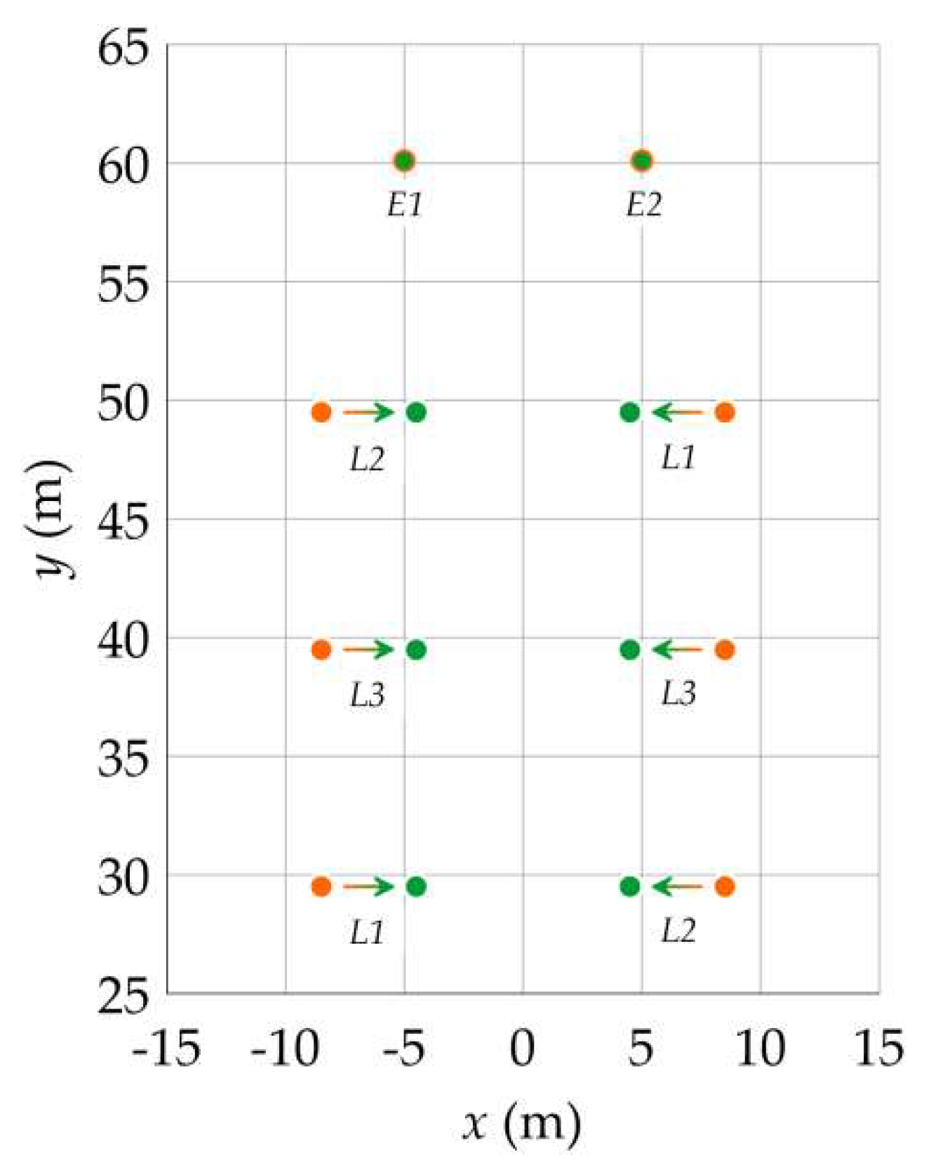
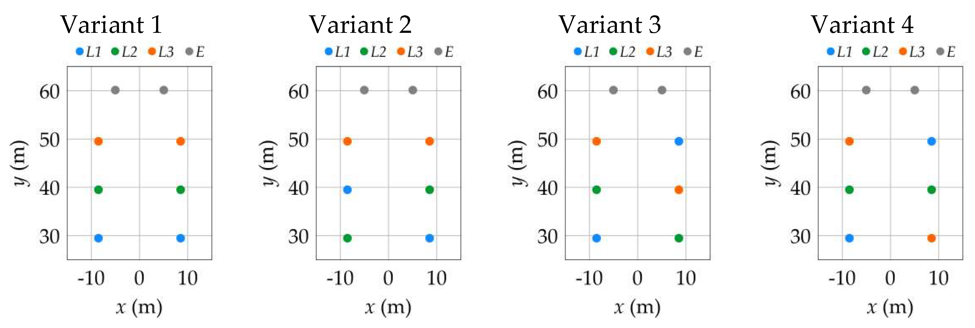
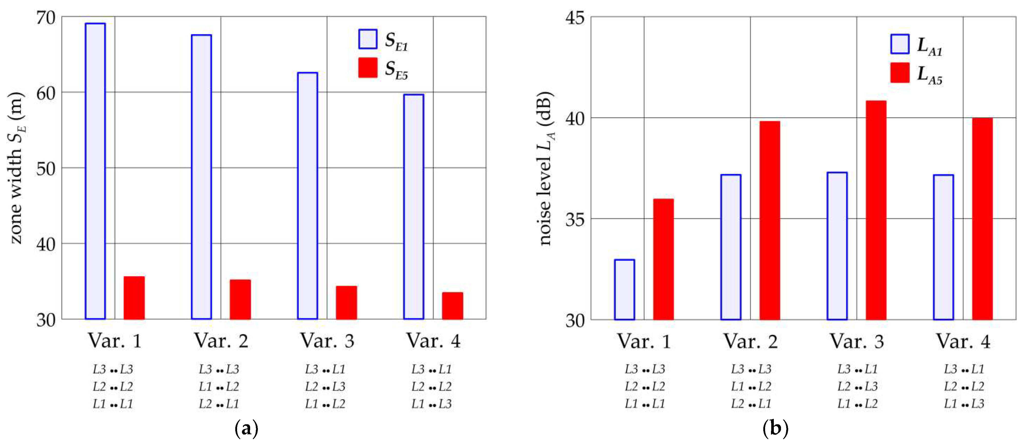
Characteristically for the double circuit lines, the electromagnetic and noise impacts depend on the phase conductor configurations in overhead line circuits. Figure 22 presents four variants of such configurations, for which zone widths S_E1, S_E5 and noise levels L_A1, L_A5 are presented in Figure 23.

The phase conductor configuration significantly affects zone width S_E1 (Figure 23a). The zone was broadest in Variant 1 (69.1 m) and the narrowest in Variant 4 (59.7 m). Shifting from the phase conductor configuration in Variant 1 to the phase conductor configuration in Variant 4 results in a reduction of zone S_E1 by 13.6%. The reduction of zone S_E5 is much smaller and is 5.9%. Unfortunately, this method of reducing zone widths is accompanied by a significant increase of noise levels L_A1, L_A5, which in the case of Variant 4 are about 4 dB higher than in Variant 1 (Figure 23b).

5. Conclusions

It follows from the research that x_p is the main parameter determining the width of the electric field influence zone. By decreasing its value we may reduce the width of the influence zones even by about 21% ÷ 31% in both single and double circuit power lines. In single circuit power lines, it is also parameter Δh_p which significantly influences the zone width. By increasing its value, a further reduction in x_p value can be achieved. On the whole, a 42% ÷ 50% reduction in the electric field influence zones can be obtained. As far as the environmental impact is concerned, the triangular phase conductor configuration turns out to be definitely more beneficial in the case of single circuit power lines than the flat one.

A slight effect on reducing the impact zones is achieved by an increase in the height of phase conductors h_p on a tower. This happens only when the distance between phase conductors and the ground is increased along the entire span. On the other hand, a change in height h_p at a constant distance of phase conductors from the ground in the middle of the span does not affect the width of the electric field influence zone.

The research has shown that the order of phases in particular circuits in double circuit power lines has a significant effect on the width of electric field influence zones. The biggest differences in their width reach over ten percent.

Unfortunately, these methods of limiting the electric field influence zones are accompanied by an increase in the corona audible noise level at the border of these zones (in extreme cases even by about 10 dB). Thus, the possibility of reducing the electric field influence zones may be conditioned by the regulations on noise intensity limits in a given area.

Unlike phase wires, the location of earth wires almost does not affect the width of electric field zones.

Research has shown that the increased number of conductors in a bundle results in a slight broadening of electric field influence zones. However, a decreased distance between the conductors in the bundle contributes to a dozen percent reduction of the width of the influence zones. It should be taken into account that the main purpose of using conductor bundles in high-voltage lines is to reduce the negative effects of corona, including noise emission. Therefore, the parameters of conductor bundles are usually selected based on other factors than the width of electric field influence zones.

Studies have shown that the proposed constructional changes can significantly reduce the width of the line’s electromagnetic impact zones. However, an increase in line construction costs must be taken into account. A precise determination of the costs of the proposed solutions is possible only for specific line designs. The authors’ design experience shows that the increase can be within a wide range (from a few % to even 40%). The presented estimates do not include the cost of acquiring an area to build the line. It should be noted that the reduction in land acquisition costs resulting from a reduction in the width of the impact zone may, in some cases, be more than the increase in construction costs resulting from a change in the line’s design.

The paper shows that the reduction in the negative environmental impact of power line influence zones is a complex issue. The originality of the solution to this problem lies in the use of complementary and experimentally verified author’s models of electric field and corona audible noise generated by power lines. The obtained results are valid not only for 400 kV lines; they also establish trends for the design and construction of high voltage transmission lines of other rated voltages (above 100 kV). Attention should be also paid to the fact that the reduction of the environmental impact of power infrastructure is an element of power energy transition processes currently taking place.

References

1. International Commission On Non-Ionizing Radiation Protection. ICNIRP Guidelines for limiting exposure to time-varying electric, magnetic and electromagnetic field (up to 300 GHz). Health Phys. 1998, 74, 494–522. [Google Scholar]
2. Council of the European Union. Council Recommendation of 12 July 1999 on the limitation of exposure of the general public to electromagnetic fields (0 Hz to 300 GHz). Off. J. Eur. Communities 1999, 42, 59–70. [Google Scholar]
3. National Institute for Public Health and the Environment. Comparison of International Policies on Electromagnetic Fields (Power Frequency and Radiofrequency Fields); National Institute for Public Health and the Environment, RIVM: Bilthoven, The Netherlands, 2017.
4. International Commission On Non-Ionizing Radiation Protection. ICNIRP Guidelines for limiting exposure to time-varying electric and magnetic fields (1 Hz to 100 kHz). Health Phys. 2010, 99, 818–836. [Google Scholar] [CrossRef] [PubMed]
5. World Health Organization. Guidelines for Community Noise; World Health Organization: Geneva, Switzerland, 1999. [Google Scholar]
6. World Health Organization. Environmental Noise Guidelines for the European Region; World Health Organization Regional Office for Europe: Copenhagen, Denmark, 2018. [Google Scholar]
7. The European Parliament and of the Council. Directive 2002/49/EC of the European Parliament and of the Council of 25 June 2002 relating to the assessment and management of environmental noise. Off. J. Eur. Communities 2002, 189, 12–26. [Google Scholar]
8. International Council on Large Electric Systems. Corona Noise Comparison of the Standard and Surface Treated Conductors Obtained with Monitoring of the Newly Erected 400 kV Line and with Corona Testing in High-Voltage Laboratory; CIGRE: Paris, France, 2016. [Google Scholar]
9. Engel, Z.; Wszołek, T. Audible noise of transmission lines caused by the corona effect: Analysis, modeling, prediction. Appl. Acoustic. 1996, 47, 149–163. [Google Scholar] [CrossRef]
10. Griffiths, D.J. Introductions to Electrodynamics, 4th ed.; Cambridge University Press: Cambridge, UK, 2017. [Google Scholar] [CrossRef]
11. El Dein, A.Z. Calculation of the electric field around the tower of the overhead lines. IEEE Trans. Power Del. 2014, 29, 899–907. [Google Scholar] [CrossRef]
12. Li, Q.; Rowland, S.M.; Shuttleworth, R. Calculating the surface potential gradient of overhead line conductors. IEEE Trans. Power Del. 2015, 30, 43–52. [Google Scholar] [CrossRef]
13. Wang, R.; Tian, J.; Wu, F.; Zhang, Z.; Liu, H. PSO/GA Combined with Charge Simulation Method for the Electric Field under Transmission Lines in 3D Calculation Model. Electronics 2019, 8, 1140. [Google Scholar] [CrossRef] [Green Version]
14. Grbić, M.; Pavlović, A. Determining the zone of influence of transmission overhead power lines from the aspect of non-ionizing radiation. RAD Conf. Proc. 2018, 3, 52–57. [Google Scholar] [CrossRef]
15. El Dein, A.Z.; Wahab, M.A.A.; Hamada, M.M.; Emmary, T.H. The effects of the span configurations and conductor sag on the electric-field distribution under overhead transmission lines. IEEE Trans. Power Del. 2010, 4, 2891–2902. [Google Scholar] [CrossRef]
16. Rácz, L.; Németh, B. Dynamic Line Rating—An Effective Method to Increase the Safety of Power Lines. Appl. Sci. 2021, 11, 492. [Google Scholar] [CrossRef]
17. Salari, J.C.; Mpalantinos, A.; Silva, J.I. Comparative analysis of 2-and 3-D methods for computing electric and magnetic fields generated by overhead transmission lines. IEEE Trans. Power Del. 2009, 1, 338–344. [Google Scholar] [CrossRef]
18. Liang, Z.; Jiang, Y.; Hong, J. Influence of complex terrains on electric field under overhead lines. In Proceedings of the 5th International Conference on Information Science and Control Engineering (ICISCE), Zhengzhou, China, 20–22 July 2018; IEEE Computer Society: Los Alamitos, CA, USA, 2018. [Google Scholar] [CrossRef]
19. International Electrotechnical Commission. IEC 61672-1:2013. Electroacoustics–Sound Level Meters–Part. 1: Specification, 2nd ed.; International Electrotechnical Commission: Geneva, Switzerland, 2013. [Google Scholar]
20. International Organization for Standardization Technical Committee ISO/TC 43/SC 1 Noise. ISO 1996-1:2016. Acoustics–Description, Measurement and Assessment of Environmental Noise–Part. 1: Basic Quantities and Assessment Procedures; International Organization for Standardization: Geneva, Switzerland, 2016. [Google Scholar]
21. International Organization for Standardization Technical Committee ISO/TC 43/SC 1 Noise. ISO 1996-2:2017. Acoustics–Description, Measurement and Assessment of Environmental Noise–Part. 2: Determination of Sound Pressure Levels; International Organization for Standardization: Geneva, Switzerland, 2017. [Google Scholar]
22. Chartier, V.L.; Sterans, R.D. Formulas for predicting audible noise from overhead high voltage AC and DC lines. IEEE Trans. Power App. Syst. 1981, 1, 121–129. [Google Scholar] [CrossRef]
23. Doyle, J.R.; LaForest, J.J.; Lauber, T.S. Electrical characteristics of EHV-UHV conductors configurations and circuit. In Transmission Line Reference Book 345 kV and Above, 2nd ed.; LaForest, J.J., Ed.; Electric Power Research Institute Inc.: Palo Alto, CA, USA, 1982; pp. 63–167. [Google Scholar]
24. International Council on Large Electric Systems, Working Group 36.01. TB 020. Interferences Produced by Corona Effect of Electric Systems; CIGRE: Paris, France, 1974. [Google Scholar]
25. International Council on Large Electric Systems, Working Group 36.01. TB 061. Addenum to CIGRE Document No. 20. Interferences Produced by Corona Effect of Electric Systems; CIGRE: Paris, France, 1996. [Google Scholar]
26. European Committee for Electrotechnical Standardization. EN-50341-1:2012 Overhead Electrical Lines Exceeding AC 1 kV–Part. 1: General Requirements–Common Specifications; CENELEC European Committee for Electrotechnical Standardization: Brussels, Belgium, 2012. [Google Scholar]
Figure 1. Exemplary images of electric and magnetic fields and widths of impact zones in the cross-section of a double circuit 400 kV line SE5, SE1–electric field exposure zone widths for admissible values 5 kV/m and 1 kV/m (authors’ research).
Energies 14 06388 g001
Figure 2. Exemplary images of electric field strength in the vicinity of a phase wire of a double circuit 400 kV line for a different number N of conductors in a bundle: (a) N = 2; (b) N = 3; (c) N = 4 (authors’ research).
Energies 14 06388 g002
Figure 3. Exemplary image of A-weighted corona audible noise level (in fair weather) in a cross-section of a 400 kV double circuit line (authors’ research).
Energies 14 06388 g003
Figure 4. Representation of an exemplary double circuit 400 kV line for the charge simulation method: (a) span wires; (b) support structure.
Energies 14 06388 g004
Figure 5. Typical spectrum of noise signal during intense corona and spectrum of noise background (own research): (a) standardized frequency A-weighted curve; (b) unweighted and A-weighted spectrum of corona noise signal (authors’ research).
Energies 14 06388 g005
Figure 6. Measurement verification of the electric field model under the double circuit 220 kV line: (a) a fragment of the span in the place of measurements; (b) comparison of the measured and calculated distribution in the cross-section of the line at a 2 m height.
Energies 14 06388 g006
Figure 7. Compared results of noise measurement (LA(90) level) and model calculations (LA(model) level) in the vicinity of double circuit 400 kV lines: (a,b) with N = 2 bundled wires; (c,d) with N = 3 bundled wires.
Energies 14 06388 g007aEnergies 14 06388 g007b
Figure 8. Analyzed parameters of 400 kV line: (a) single circuit line; (b) double circuit line; (c) phase wire.
Energies 14 06388 g008
Figure 9. Configuration of a single circuit 400 kV line (a) and a double circuit 400 kV line (b).
Energies 14 06388 g009
Figure 10. Conductor profiles of outer phases of a single circuit 400 kV line: (a) constant sag fP = fE = 13.5 m; (b) variable sag fP = fE = var.
Energies 14 06388 g010
Figure 11. Variability of zone widths sE1 (a,c) and sE5 (b,d) along the span for constant (a,b) and variable (c,d) sag of conductors in a single circuit 400 kV line.
Energies 14 06388 g011
Figure 12. Influence of height hP on zone widths SE1 and SE5 (a) and corona audible noise level LA1 and LA5 on the boundary of zones SE1 andSE5 (b).
Energies 14 06388 g012
Figure 13. Range of parameter xP values in a single circuit 400 kV line: (a) constant position of earth wires xE, ∆hE = const; (b) variable position of earth wires xE, ∆hE = var.
Energies 14 06388 g013
Figure 14. Influence of distance xP on zone widths SE1 and SE5 (a) and noise level LA1 and LA5 on the boundary of zones SE1 and SE5 (b).
Energies 14 06388 g014
Figure 15. Reconfiguration of flat conductor configuration to triangular conductor configuration in a single circuit 400 kV line: (a) variable position of the outermost phase conductors xP = var; (b) constant position of outermost phase conductors xP = const.
Energies 14 06388 g015
Figure 16. Influence of distance hP on zone widths SE1 and SE5 (a) and noise levels LA1 and LA5 on the boundary of zones SE1 and SE5 (b).
Energies 14 06388 g016
Figure 17. Analyzed bundled conductors: (a) changed number of conductors N; (b) change of distance b.
Energies 14 06388 g017
Figure 18. Influence of number N of sub-conductors in a bundle and distance ΔhP on zone widths SE1, SE5 (a) and noise levels LA1, LA5 (b).
Energies 14 06388 g018
Figure 19. Influence of sub-conductor distance b in a bundle on zone widths SE1 and SE5 (a) and noise level LA1 and LA5 on the boundary of zones SE1 and SE5 (b).
Energies 14 06388 g019
Figure 20. Range of parameter xP on a double circuit 400 kV line—constant position of earth wires xE, ΔhE = const and a constant vertical distance ΔhP = const.
Energies 14 06388 g020
Figure 21. Influence of distance xP on zones width SE1 and SE5 (a) and noise level LA1 and LA5 on the boundary of zones SE1 and SE5 for a double circuit 400 kV line (b).
Energies 14 06388 g021
Figure 22. Considered variants of phase conductor configurations in a double circuit 400 kV line.
Energies 14 06388 g022
Figure 23. Influence of the phase conductor configuration in a double circuit 400 kV line on zone widths SE1 and SE5 (a) and noise level LA1 and LA5 on the boundary of zones SE1 and SE5 (b).
Energies 14 06388 g023