
Enhancing Stability and Robustness of State-of-Charge Estimation for Lithium-Ion Batteries by Using Improved Adaptive Kalman Filter Algorithms

Abstract
:1. Introduction
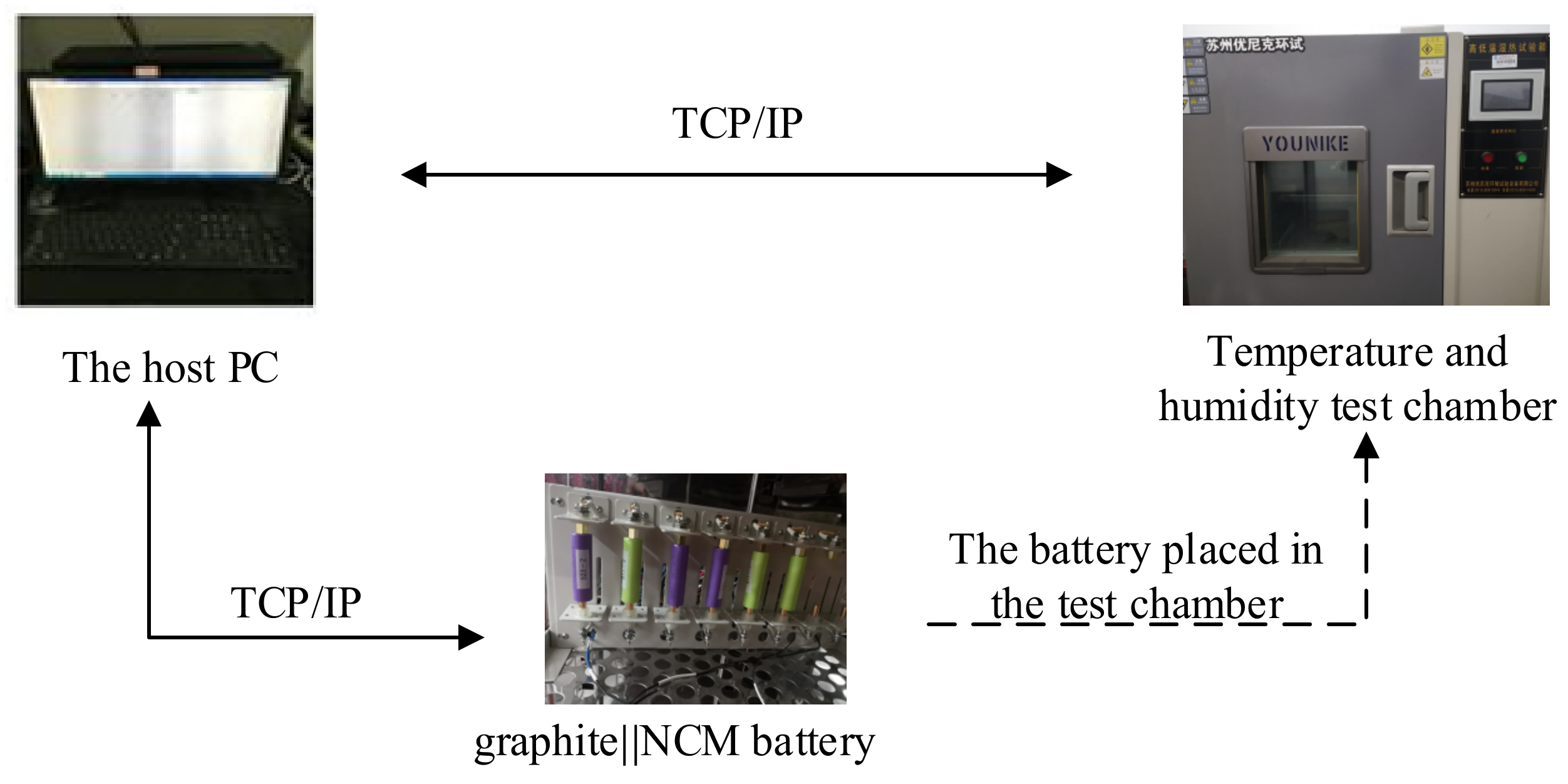
2. Experiments
3. Description of the Adaptive Kalman Filter
3.1. Adaptive Sage-Husa Kalman Filter
3.2. Adaptive Kalman Filter Based on the Maximum Likelihood Criterion
3.3. State-of-Charge Estimation
4. Results and Discussion
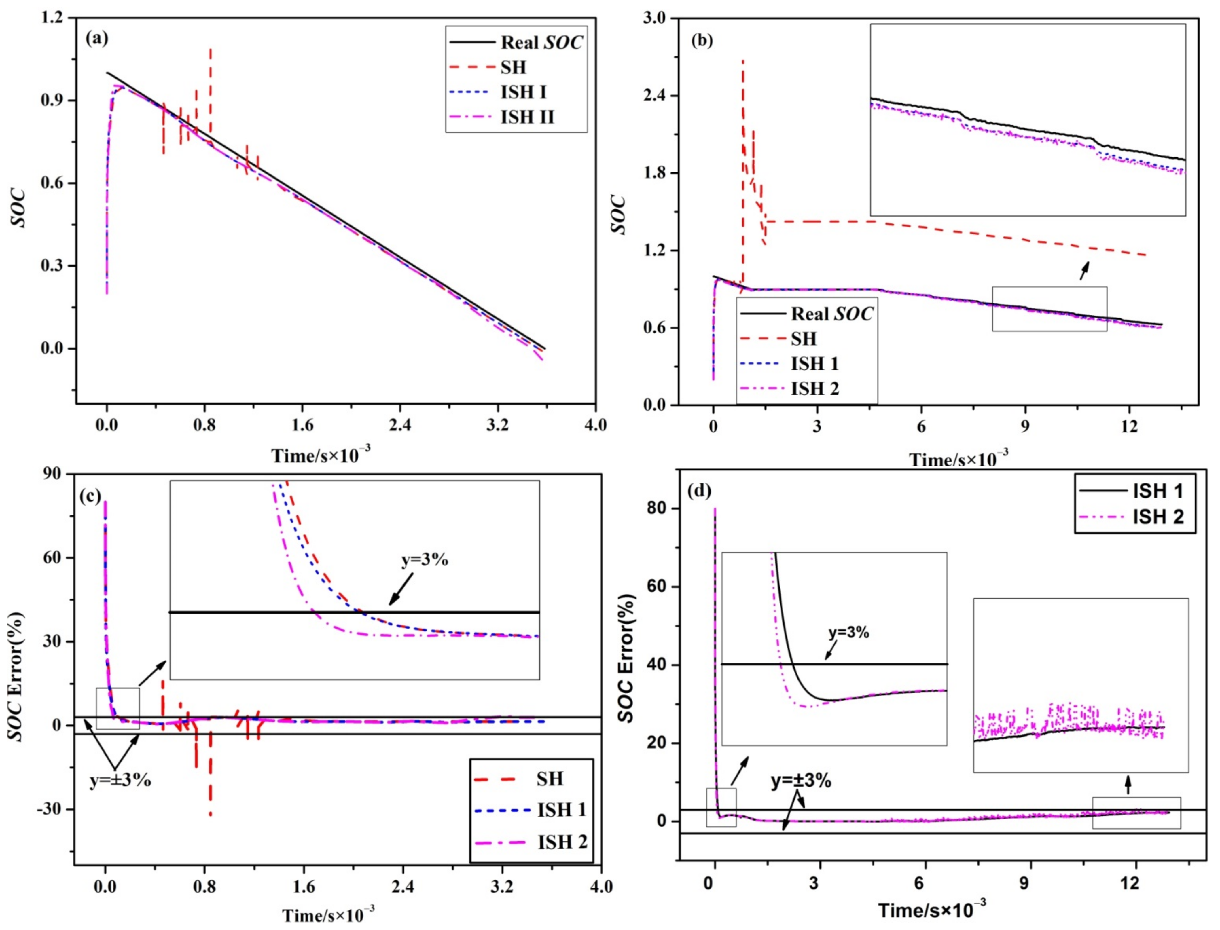
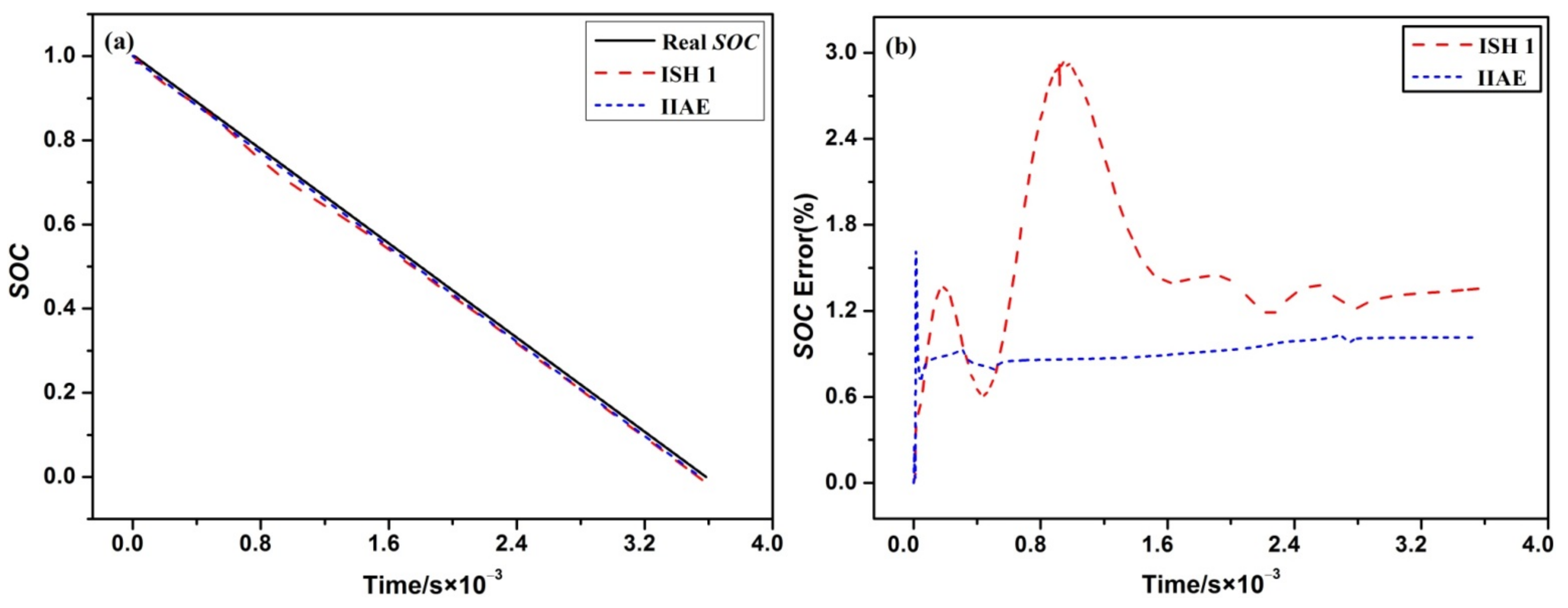
4.1. State-of-Charge Estimation Using the Improved Sage-Husa Algorithm
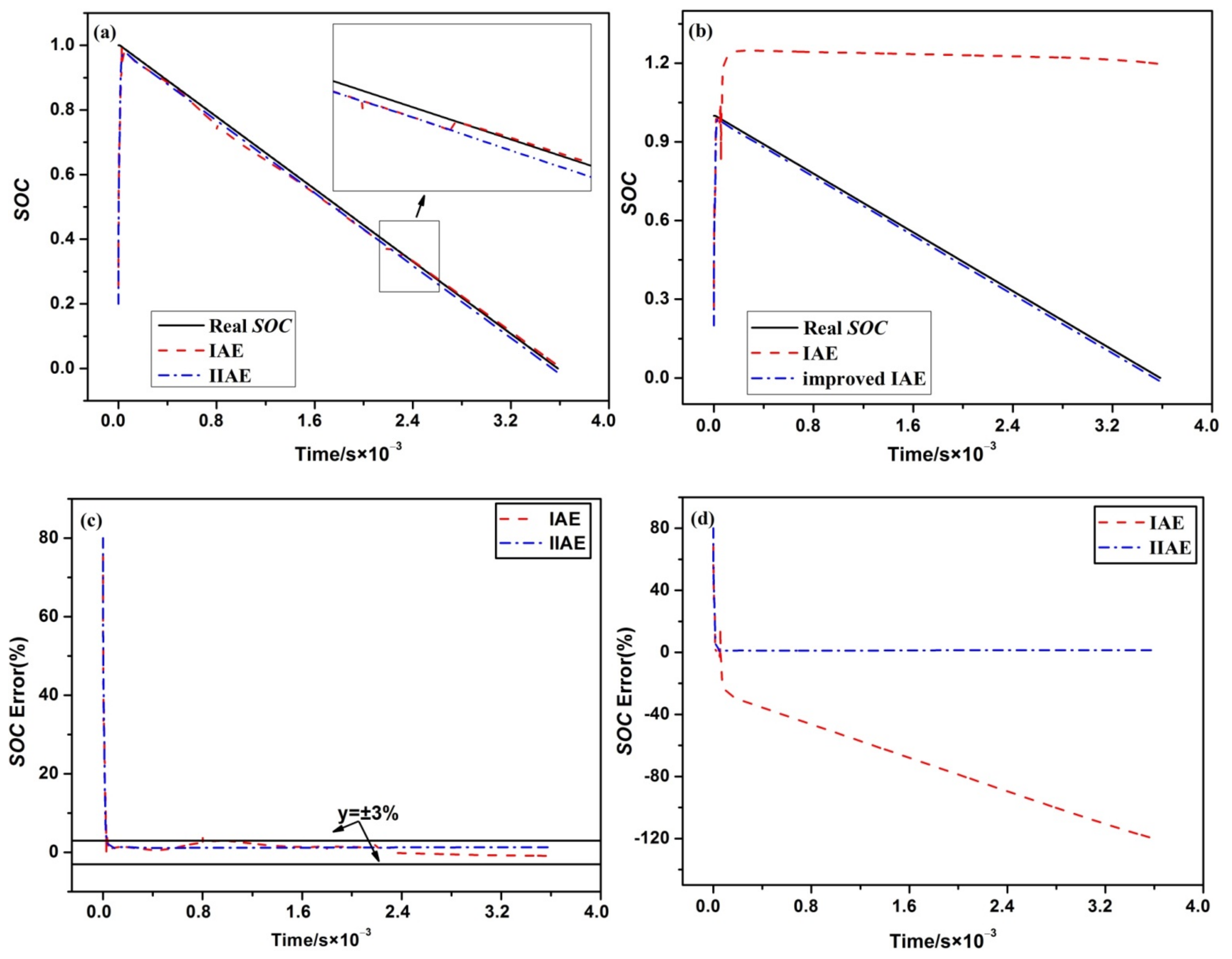
4.2. Estimation Using the Improved Maximum Likelihood Criterion Algorithm
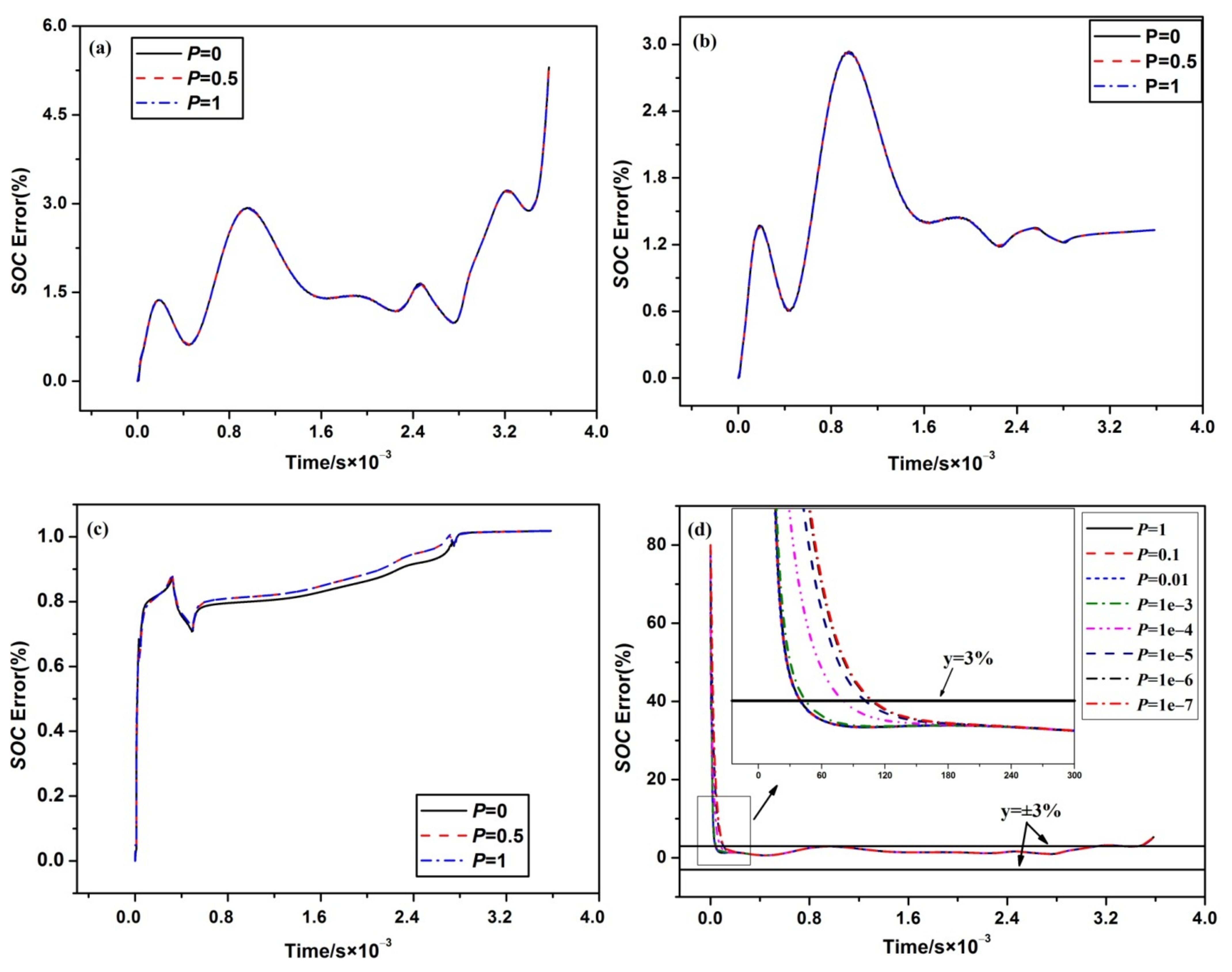
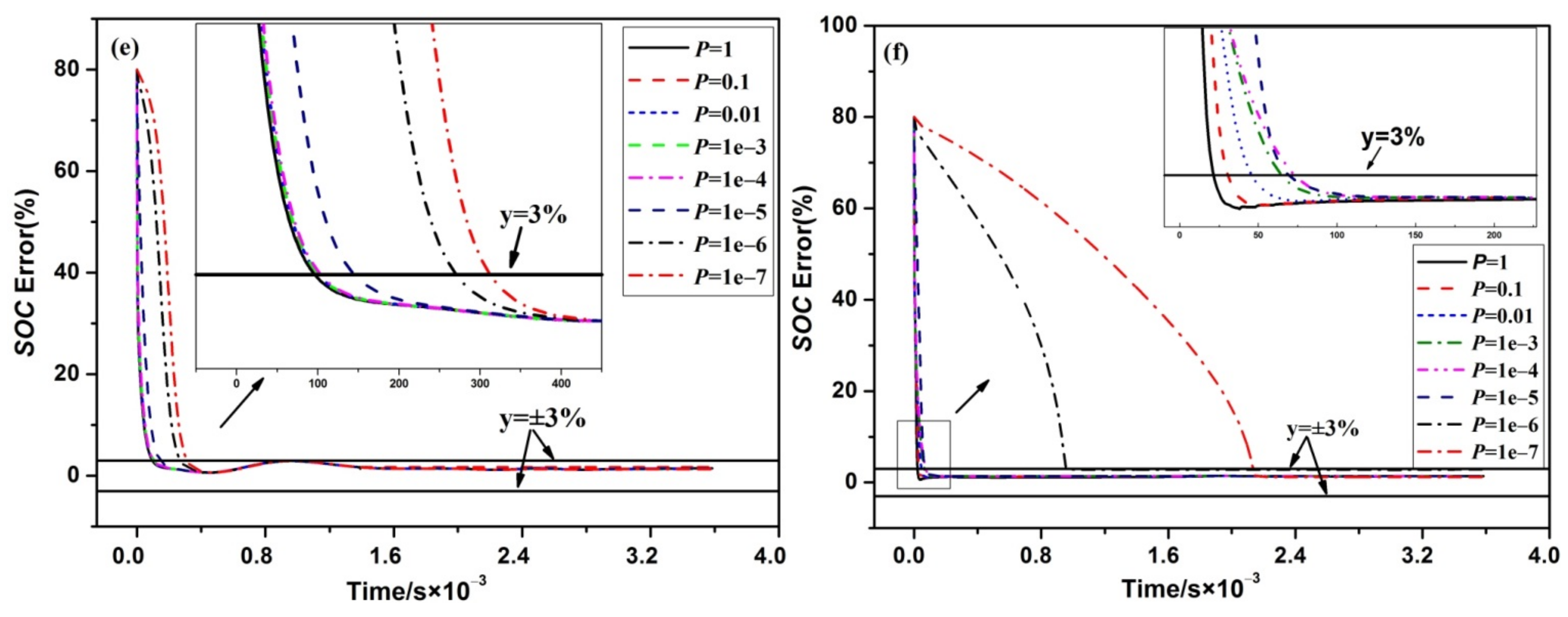
4.3. Effects of the State Variable Error Covariance on the Estimation
4.4. Effects of the Noise Covariance on the Estimation
5. Conclusions
Author Contributions
Funding
Institutional Review Board Statement
Informed Consent Statement
Data Availability Statement
Conflicts of Interest
Abbreviations
| AEKF | Adaptive extend Kalman filter |
| BMS | Battery Management System |
| CCD | Constant current discharge |
| CDKF | Central difference Kalman filter |
| DEKF | Dual extended Kalman filter |
| DP | Dual polarization |
| EV | Electric vehicles |
| EKF | Extend Kalman filter method |
| FUDS | Federal Urban Driving Schedule |
| HPPC | Hybrid pulse power characteristic |
| IIAE | Improved innovation-based adaptive estimation |
| ISH I | Improved Sage-Husa 1 |
| ISH II | Improved Sage-Husa 2 |
| PNGV | Partnership for a new generation of vehicles |
| RMSE | Root mean square error |
| SOC | State of charge |
| SOP | State of power |
| SRUKF | Square-root unscented Kalman filter |
| UKF | Unscented Kalman filter |
| UDDS | Urban Dynamometer Driving Schedule |
List of Notations
| b | Forgetting factor |
| covariance | |
| The rated capacity of the battery | |
| Concentration capacitance | |
| Electrochemical capacitance | |
| covariance | |
| Adaptive factors | |
| Kalman gain | |
| M | Moving average window length |
| The initial error covariance | |
| The auto-covariance of SOC | |
| covariance matrix | |
| covariance matrix | |
| Ohmic internal resistance | |
| Concentration resistance | |
| Electrochemical resistance | |
| The innovation as a residual sequence | |
| Open circuit voltage | |
| The terminal voltage of the battery | |
| Concentration polarization voltage | |
| Electrochemical polarization voltage | |
| System excitation | |
| Measurement noise | |
| State vector | |
| Filtered value of the state variable | |
| Predicted value of the state variable | |
| Predicted value of the measured variable | |
| Process noise | |
| The discharge efficiency |
References
- Karnama, A.; Resende, F.O.; Lopes, J.A.P. Optimal management of battery charging of electric vehicles: A new microgrid feature. In Proceedings of the 2011 IEEE Trondheim PowerTech, Trondheim, Norway, 19–23 June 2011; IEEE: Piscataway, NJ, USA, 2011; pp. 1–8. [Google Scholar]
- Zhu, J.; Knapp, M.; Liu, X.; Yan, P.; Dai, H.; Wei, X.; Ehrenberg, H. Low-Temperature Separating Lithium-Ion Battery Interfacial Polarization Based on Distribution of Relaxation Times (DRT) of Impedance. IEEE Trans. Transp. Electrif. 2021, 7, 410–421. [Google Scholar] [CrossRef]
- Liu, C.; Wang, Y.; Chen, Z. Degradation model and cycle life prediction for lithium-ion battery used in hybrid energy storage system. Energy 2019, 166, 796–806. [Google Scholar] [CrossRef]
- Jiang, B.; Dai, H.; Wei, X. Incremental capacity analysis based adaptive capacity estimation for lithium-ion battery considering charging condition. Appl. Energy 2020, 269, 115074. [Google Scholar] [CrossRef]
- Li, J.; Lai, Q.; Wang, L.; Lyu, C.; Wang, H. A method for SOC estimation based on simplified mechanistic model for LiFePO4 battery. Energy 2016, 114, 1266–1276. [Google Scholar] [CrossRef]
- Cheng, K.W.E.; Divakar, B.P.; Wu, H.; Ding, K.; Ho, H.F. Battery-Management System (BMS) and SOC Development for Electrical Vehicles. IEEE Trans. Veh. Technol. 2011, 60, 76–88. [Google Scholar] [CrossRef]
- Dai, H.; Jiang, B.; Hu, X.; Lin, X.; Wei, X.; Pecht, M. Advanced battery management strategies for a sustainable energy future: Multilayer design concepts and research trends. Renew. Sustain. Energy Rev. 2021, 138, 110480. [Google Scholar] [CrossRef]
- Zhao, X.; Cai, Y.; Yang, L.; Deng, Z.; Qiang, J. State of charge estimation based on a new dual-polarization-resistance model for electric vehicles. Energy 2017, 135, 40–52. [Google Scholar] [CrossRef]
- Xia, B.; Chen, C.; Tian, Y.; Wang, M.; Sun, W.; Xu, Z. State of charge estimation of lithium-ion batteries based on an improved parameter identification method. Energy 2015, 90, 1426–1434. [Google Scholar] [CrossRef]
- Zhu, Q.; Xu, M.; Liu, W.; Zheng, M. A state of charge estimation method for lithium-ion batteries based on fractional order adaptive extended kalman filter. Energy 2019, 187, 115880. [Google Scholar] [CrossRef]
- Tong, C.H.; Barfoot, T.D. A Comparison of the EKF, SPKF, and the Bayes Filter for Landmark-Based Localization. In Proceedings of the 2010 Canadian Conference on Computer and Robot Vision, Ottawa, ON, Canada, 31 May–2 June 2010; pp. 199–206. [Google Scholar]
- Plett, G.L. Extended Kalman filtering for battery management systems of LiPB-based HEV battery packs: Part 2. Modeling and identification. J. Power Sources 2004, 134, 262–276. [Google Scholar] [CrossRef]
- Sadhu, S.; Mondal, S.; Srinivasan, M.; Ghoshal, T.K. Sigma point Kalman filter for bearing only tracking. Signal Process. 2006, 86, 3769–3777. [Google Scholar] [CrossRef]
- Plett, G.L. Sigma-point Kalman filtering for battery management systems of LiPB-based HEV battery packs: Part 2: Simultaneous state and parameter estimation. J. Power Sources 2006, 161, 1369–1384. [Google Scholar] [CrossRef]
- Jokić, I.; Zečević, Ž.; Krstajić, B. State-of-charge estimation of lithium-ion batteries using extended Kalman filter and unscented Kalman filter. In Proceedings of the 2018 23rd International Scientific-Professional Conference on Information Technology (IT), Zabljak, Montenegro, 19–24 February 2018; pp. 1–4. [Google Scholar]
- Merwe, R. Sigma-Point Kalman Filters for Probabilistic Inference in Dynamic State-Space Models. Ph.D. Thesis, Oregon Health & Science University, Portland, OR, USA, 2004. [Google Scholar]
- Charkhgard, M.; Farrokhi, M. State-of-Charge Estimation for Lithium-Ion Batteries Using Neural Networks and EKF. IEEE Trans. Ind. Electron. 2010, 57, 4178–4187. [Google Scholar] [CrossRef]
- Sepasi, S.; Ghorbani, R.; Liaw, B.Y. A novel on-board state-of-charge estimation method for aged Li-ion batteries based on model adaptive extended Kalman filter. J. Power Sources 2014, 245, 337–344. [Google Scholar] [CrossRef]
- Xiong, R.; He, H.; Sun, F.; Zhao, K. Evaluation on State of Charge Estimation of Batteries With Adaptive Extended Kalman Filter by Experiment Approach. IEEE Trans. Veh. Technol. 2013, 62, 108–117. [Google Scholar] [CrossRef]
- Tian, Y.; Chen, Z.; Yin, F. Distributed IMM-Unscented Kalman Filter for Speaker Tracking in Microphone Array Networks. IEEE/ACM Trans. Audio Speech Lang. Process. 2015, 23, 1637–1647. [Google Scholar] [CrossRef]
- Zhao, L. Nonlinear System Filtering Theory; National Defense Industry Press: Beijing, China, 2012. [Google Scholar]
- Xiong, R.; He, H.; Sun, F.; Liu, X.; Liu, Z. Model-based state of charge and peak power capability joint estimation of lithium-ion battery in plug-in hybrid electric vehicles. J. Power Sources 2013, 229, 159–169. [Google Scholar] [CrossRef]
- Xiong, R.; Sun, F.; He, H.; Nguyen, T.D. A data-driven adaptive state of charge and power capability joint estimator of lithium-ion polymer battery used in electric vehicles. Energy 2013, 63, 295–308. [Google Scholar] [CrossRef]
- Partovibakhsh, M.; Liu, G. An Adaptive Unscented Kalman Filtering Approach for Online Estimation of Model Parameters and State-of-Charge of Lithium-Ion Batteries for Autonomous Mobile Robots. IEEE Trans. Control Syst. Technol. 2014, 23, 357–363. [Google Scholar] [CrossRef]
- Junping, W.; Jingang, G.; Lei, D. An adaptive Kalman filtering based State of Charge combined estimator for electric vehicle battery pack. Energy Convers. Manag. 2009, 50, 3182–3186. [Google Scholar] [CrossRef]
- Liu, S.; Cui, N.; Zhang, C. An Adaptive Square Root Unscented Kalman Filter Approach for State of Charge Estimation of Lithium-Ion Batteries. Energies 2017, 10, 1345. [Google Scholar] [CrossRef] [Green Version]
- Fan, K.; Zhao, W.; Liu, J.Y. Adaptive Filtering Algorithm for SINS/GPS Integrated Navigation System; Avion Technologies: Schaumburg, IL, USA, 2008. [Google Scholar]
- Mohamed, A.H.; Schwarz, K.P. Adaptive Kalman Filtering for INS/GPS. J. Geod. 1999, 73, 193–203. [Google Scholar] [CrossRef]
- Sunahara, Y.; Yamashita, K. An Approximate Method of State Estimation for Nonlinear Dynamical Systems with State-Dependent Noise. Int. J. Control 1970, 11, 957–972. [Google Scholar] [CrossRef]
- Bucy, R.S.; Senne, K.D. Digital synthesis of non-linear filters. Automatica 1971, 7, 287–298. [Google Scholar] [CrossRef]
- Sage, A.; Husa, G. Algorithms for sequential adaptive estimation of prior statistics. In Proceedings of the 1969 IEEE Symposium on Adaptive Processes (8th) Decision and Control, University Park, PA, USA, 17–19 November 1969; IEEE: Piscataway, NJ, USA, 1969; p. 61. [Google Scholar]
- Deng, Z. Dynamic prediction of the oil and water outputs in oil field. Acta Autom. Sin. 1983, 9, 121–126. [Google Scholar]
- Wei, W.; Qin, Y.-Y.; Zhang, X.-D.; Zhang, Y.-C. Amelioration of the Sage-Husa algorithm. J. Chin. Inert. Technol. 2012, 6, 678–686. [Google Scholar]
- Mehra, R.K. Approaches to adaptive filtering. Autom. Control IEEE Trans. 1972, 17, 693–698. [Google Scholar] [CrossRef]
- Hongwei, B.; Zhihua, J.; Weifeng, T. IAE-adaptive Kalman filter for INS/GPS integrated navigation system. J. Syst. Eng. Electron. 2006, 17, 502–508. [Google Scholar] [CrossRef]
- Hentunen, A.; Lehmuspelto, T.; Suomela, J. Time-Domain Parameter Extraction Method for Thévenin-Equivalent Circuit Battery Models. IEEE Trans. Energy Convers. 2014, 29, 558–566. [Google Scholar] [CrossRef]
- He, H.; Xiong, R.; Guo, H.; Li, S. Comparison study on the battery models used for the energy management of batteries in electric vehicles. Energy Convers. Manag. 2012, 64, 113–121. [Google Scholar] [CrossRef]
- Tan, X. Applied Technology and Advanced Theories; Sun Yat-sen university press: Guangzhou, China, 2014. [Google Scholar]
- Chen, B.; Jiang, H.; Chen, X.; Li, H. Robust state-of-charge estimation for lithium-ion batteries based on an improved gas-liquid dynamics model. Energy 2021, 238, 122008. [Google Scholar] [CrossRef]
- Ee, Y.J.; Tey, K.S.; Lim, K.S.; Shrivastava, P.; Ahmad, H. Lithium-Ion Battery State of Charge (SOC) Estimation with Non-Electrical parameter using Uniform Fiber Bragg Grating (FBG). J. Energy Storage 2021, 40, 102704. [Google Scholar] [CrossRef]
- Liu, S.; Wang, J.; Liu, Q.; Tang, J.; Liu, H.; Fang, Z.-J. Deep-Discharging Li-Ion Battery State of Charge Estimation Using a Partial Adaptive Forgetting Factors Least Square Method. IEEE Access 2019, 7, 47339–47352. [Google Scholar] [CrossRef]


| Step 2 Computation: for k = 1, 2, 3… Time update: | |
| Kalman gain: | |
| Measurement update: | |
| Adaptive factor: | |
| Process noise covariance and measurement noise covariance update: | |
| ISH I: | |
| ISH II: | |
| Step 2 Computation: For k = 1, 2, 3… Time update: |
| Kalman gain: |
| Measurement update: |
| Judgement: |
| If (estimated step size < M) |
| Else |
| Process noise covariance and measurement noise covariance update: |
| Algorithm | Operating Conditions | Max(%) | Mean(%) | RMSE(%) | Convergence Time/s |
|---|---|---|---|---|---|
| SH | CCD | 16.72 | 1.652 | 3.693 | 98 |
| ISH I | 2.929 | 1.562 | 3.311 | 96 | |
| ISH II | 5.345 | 1.856 | 3.603 | 63 | |
| ISH I | FUDS | 2.306 | 0.822 | 1.857 | 87 |
| ISH II | 3.257 | 0.952 | 2.009 | 59 |
| Algorithm | Max(%) | Mean(%) | RMSE(%) | Convergence Time/s |
|---|---|---|---|---|
| IAE (M = 100) | 4.218 | 0.841 | 2.982 | 36 |
| IIAE (M = 100) | 1.377 | 1.234 | 2.857 | 29 |
| IIAE (M = 10) | 1.438 | 1.263 | 2.828 | 21 |
| Initial SOC | Test | Algorithm | Max (%) | Mean(%) | RMSE(%) | Convergence Time/s |
|---|---|---|---|---|---|---|
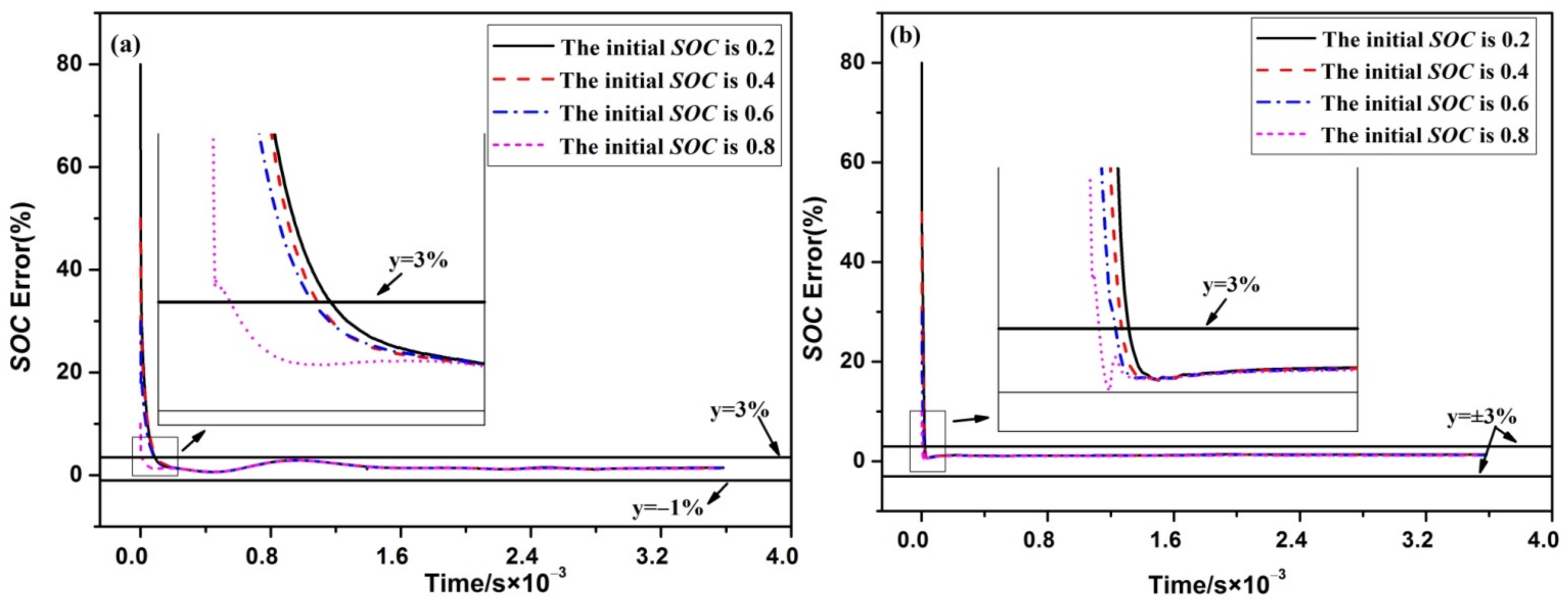
| SOC = 0.2 | CCD | ISH I | 2.929 | 1.557 | 3.312 | 109 |
| IIAE | 1.437 | 1.264 | 2.828 | 22 | ||
| SOC = 0.4 | CCD | ISH I | 2.919 | 1.548 | 3.327 | 97 |
| IIAE | 1.383 | 1.213 | 2.245 | 19 | ||
| SOC = 0.6 | CCD | ISH I | 2.921 | 1.544 | 2.5 | 92 |
| IIAE | 1.363 | 1.206 | 1.68 | 15 | ||
| SOC = 0.8 | CCD | ISH I | 2.952 | 1.514 | 1.721 | 16 |
| IIAE | 1.354 | 1.154 | 1.302 | 6 | ||
| 50% error | DST | Ref. [39] | 2.49 | 0.63 | - | 6 |
| No error | nonstandard | Ref. [40] | - | 0.12 | 3.50 | - |
| No error | B-DST | Ref. [41] | 2 | 1.24 | 1.35 | - |
Publisher’s Note: MDPI stays neutral with regard to jurisdictional claims in published maps and institutional affiliations. |
© 2021 by the authors. Licensee MDPI, Basel, Switzerland. This article is an open access article distributed under the terms and conditions of the Creative Commons Attribution (CC BY) license (https://creativecommons.org/licenses/by/4.0/).
Share and Cite
Zhang, F.; Yin, L.; Kang, J. Enhancing Stability and Robustness of State-of-Charge Estimation for Lithium-Ion Batteries by Using Improved Adaptive Kalman Filter Algorithms. Energies 2021, 14, 6284. https://doi.org/10.3390/en14196284
Zhang F, Yin L, Kang J. Enhancing Stability and Robustness of State-of-Charge Estimation for Lithium-Ion Batteries by Using Improved Adaptive Kalman Filter Algorithms. Energies. 2021; 14(19):6284. https://doi.org/10.3390/en14196284
Chicago/Turabian StyleZhang, Fan, Lele Yin, and Jianqiang Kang. 2021. "Enhancing Stability and Robustness of State-of-Charge Estimation for Lithium-Ion Batteries by Using Improved Adaptive Kalman Filter Algorithms" Energies 14, no. 19: 6284. https://doi.org/10.3390/en14196284
APA StyleZhang, F., Yin, L., & Kang, J. (2021). Enhancing Stability and Robustness of State-of-Charge Estimation for Lithium-Ion Batteries by Using Improved Adaptive Kalman Filter Algorithms. Energies, 14(19), 6284. https://doi.org/10.3390/en14196284