On the Impact of GDP per Capita, Carbon Intensity and Innovation for Renewable Energy Consumption: Worldwide Evidence

Abstract

The mitigation of climate change through ambitious greenhouse gases emission reduction targets constitutes a current priority at world level, reflected in international, regional and national agendas. Within the common framework for global climate action, an increased reliance on renewable energy sources, which would assist countries to reduce energy imports and cut fossil fuel use, emerged as the solution towards achieving worldwide energy security and sustainability through carbon-neutrality. As such, this study is aimed to investigate the heterogeneous effects of relevant economic and environmental driving factors for renewable energy consumption (REC) that emerge from current policy objectives (GDP per capita, carbon intensity, and research and development) through an empirical analysis of a wide panel of 94 countries, and five income-based subpanels, over the 1995–2019 period, by using heterogeneous panel data fixed-effects estimation techniques (static and dynamic) with robust Driscoll–Kraay standard errors. The results unambiguously indicate that CO₂ intensity has a significant mitigating effect on REC at world level, and this relationship is stronger for low-income and very high-income countries. Moreover, GDP per capita promotes REC when it surpasses the 5000 USD threshold, whereas research and development is a major contributor to increase in renewable energy consumption in very high-income countries. As such, for the policy makers, it is necessary to consider the heterogeneity of the drivers of REC in order to issue effective and congruent policies. The effective employment of post-COVID-19 recovery funds constitutes a timely, ideal occasion.

1. Introduction

Over the last decades, the whole world has become increasingly aware of the importance of immediate and significant climate change actions for a sustainable future [1].

At a governmental level, one of the paramount manifestations of this common understanding is represented by the Paris Agreement, signed on 12 December 2015 by 195 nations and ratified by 190 countries of the United Nations Framework Convention on Climate Change (UNFCCC) as of January 2021, which establishes a common framework for global climate action. Common efforts towards the mitigation of climate change through ambitious greenhouse gases emission reduction targets are also currently reflected in other international, regional and national agendas (i.e., United Nations’ 2030 Agenda for Sustainable Development, the European Green Deal, etc.).

However, the main challenge that economies face is reaching their environmental targets while minimizing or eliminating costs in terms of economic prosperity [2]. Nonetheless, the relationship between income and environmental quality remains puzzling [3]. According to the Environmental Kuznets Curve (EKC) hypothesis, pollution increases with the economic growth, until some threshold level of income is reached and emissions start declining, thus suggesting an inverted U-shaped relationship between environmental degradation and income. However, studies that investigate the existence of the EKC in different countries over different time periods found mixed results [4], and consequently the subject of how economic growth affects the environmental quality (i.e., the shape of the environmental Kuznets curve) remains controversial [5].

Within the economic prosperity-environmental quality nexus, an increased reliance on “green energy” sources, which implies increased renewable energy production and consumption, emerged as an effective approach that governments may use to not only reduce pollution and reach their emission mitigation targets, but more importantly to also spur economic growth [6].

Renewable energy sources generate significantly less global warming emissions than fossil fuels such as coal, oil, and natural gas (for example, while on one hand natural gas releases between 0.6 and 2 pounds of carbon dioxide equivalent per kilowatt-hour (CO₂E/kWh) and coal emits between 1.4 and 3.6 pounds of CO₂E/kWh, on the other hand the global warming emissions associated with renewable energy sources are minimal: i.e., wind is responsible for only 0.02 to 0.04 pounds of CO₂E/kWh on a life-cycle basis, solar releases 0.07 to 0.2 pounds of CO₂E/kWh, geothermal 0.1 to 0.2 pounds of CO₂E/kWh, and hydroelectric between 0.1 and 0.5 pounds of CO₂E/kWh. Emissions produced by biomass can vary widely depending on the specific resource and whether or not it is sustainably sourced and harvested: https://www.ucsusa.org/resources/benefits-renewable-energy-use, accessed on 20 June 2021). These figures are also backed by empirical findings, which consistently confirm that switching from unsustainable fossil fuels to sustainable “green” energy sources significantly reduces global greenhouse gas emissions ([7,8,9,10,11,12], among others). In addition, countries do not necessarily incur economic costs when they increase renewable sources in their energy mix [13,14]. 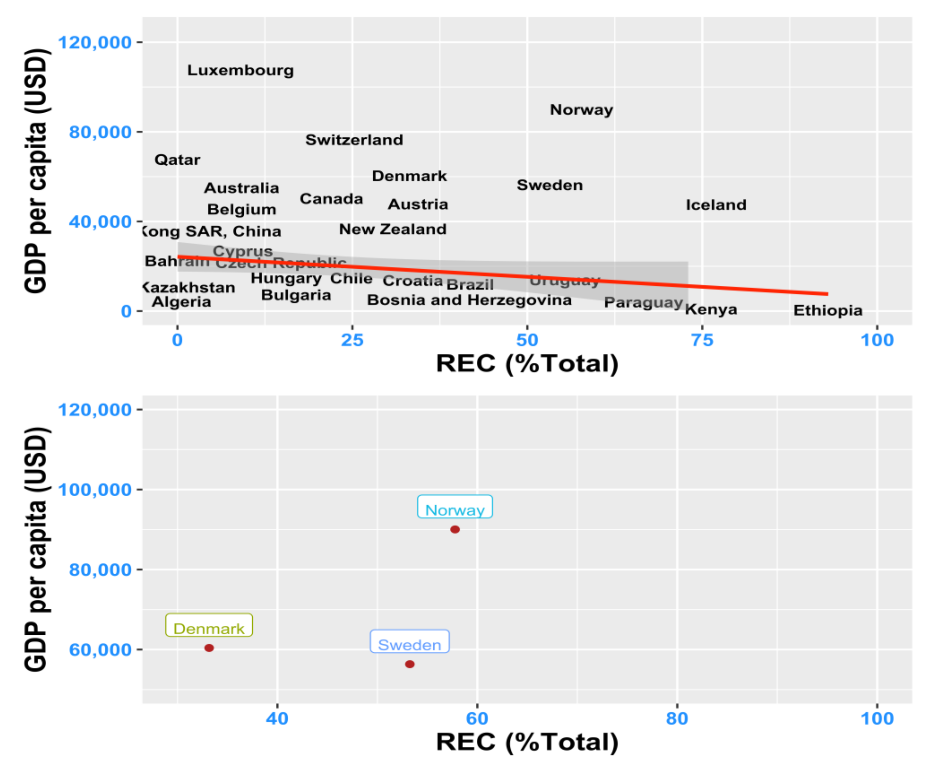Indeed, while Figure 1 (Panel A) reflects that the increasing share of renewable energy to the total energy is generally negatively related to economic income at world level, suggesting that countries must incur some economic costs in order to achieve carbon neutrality and hence a sustainable development, it also reflects (Panel B) some notable success stories of rich countries that contradict this relationship (i.e., Norway, Sweden, Denmark) and that should be first understood and subsequently followed.

Unsurprisingly, international agencies and governments have focused on issuing energy policies increasingly focused on the development of renewables [15,16].

However, renewable energy still only accounts for approximately a fifth of worldwide electricity generation [17]. Moreover, governmental subsidies that support the coal, gas, and oil industries remain large at world level [18]. This incongruence between policy objectives and current global reality needs to be overcome not only for achieving international common priorities, but also more importantly for attaining worldwide energy security and sustainable development.

The obvious solution to increasing global renewable energy consumption is first to understand its driving factors and further to promote it through an efficient mix of congruent policies. As such, the investigation of explanatory factors for renewable energy is a timely research topic, further motivated by at least four important reasons. First, the share of modern renewable energy in global final energy consumption should globally increase to 28% by 2030 and to 66% by 2050, should the targets set by current international agendas be met [19]. Second, the never-before seen disruptions on the crude oil markets during the onset of the COVID-19 pandemic, which confirmed that countries relying on a high fossil fuel share in their energy mix, or on energy intensive industrial production, are more vulnerable to oil price shocks [20,21] and hence that increasing renewable energy is a key factor for achieving the desired energy security. In addition, the International Energy Agency (IEA)’s Global Energy Review 2020 [22] projected renewables to be the only energy source to grow in 2020 compared to 2019, in contrast to all fossil fuels and nuclear, while a subsequent IEA’s report [23] attested that renewables are more resilient than fossil-fuels, being the only energy source for which demand increased in 2020 despite the pandemic, while consumption of all other fuels declined. Third, post-COVID-19 recovery funds need to be efficiently directed to drive an inclusive and sustainable economic recovery [24]. Lastly, there is currently a research gap in what driving factors for renewable energy are concerned [25].

All these factors motivate our study. Hence, the main goal of this research is to investigate how renewable energy consumption (REC) can be increased at world level thorough the identification of its potential drivers, both economic and environmental, and thus to further analyze whether the carbon intensity, and/or the economic income of a country and its propensity for innovation are driving renewable energy consumption, and whether distinct, country/group-specific policies are needed accordingly. The results of this research thus have important implications for future policy issuance and contribute on promoting renewable energies together with optimal macroeconomic policies.

This paper adds to the extant literature by offering an answer to its main research question (i.e., the identification of policy relevant driving factors for renewable energy consumption), which is further divided in four relevant sub-questions that are answered individually through robust panel data methods applied on a wide sample of 94 countries for the period 1995–2019:

(1)

Is there a significant relationship between the economic development (GDP per capita) of a country and its preference towards renewable energy consumption?

(2)

Is there a significant relationship between a country’s initiative towards innovation (as proxied by its public R&D expenditure) and its renewable energy consumption?

(3)

Is there a significant relationship between the level of carbon intensity and the consumption of renewable energy?

(4)

Is there a differential impact of relevant driving factors for renewable energy consumption according to a country’s inclusion in a given income category, at world level?

As such, we also examine these relationships for five homogenous groups of countries, delineated on the basis of the income level: very high-, high-, middle high-, middle low- and low-income subpanels. This investigation thus allows us to answer the above mentioned forth research sub-question by assessing any group-specific features in terms of the impact that potential driving factors have on renewable energy consumption, and hence to assess the necessity for targeted energy policies.

The remainder of this paper is organized as follows: Section 2 reviews the related extant literature; Section 3 presents the data; Section 4 contains some exploratory analysis of data, estimates relevant prior tests for the empirical models, and also presents the methods and the overall conceptual framework of the investigation; Section 5 presents the estimation results, followed by a discussion of results in Section 6; finally, Section 7 offers the conclusions, as well as, policy implications.

2. Literature Review

The causal relationship from increased renewable energy production and or/utilization to decreasing greenhouse gas emissions has been repeatedly validated by prior research endeavors. For example, [7] perform an analysis on 29 OECD countries and show that, renewable energy consumption has a negative and significant effect on CO₂ emissions, whereas non-renewable energy consumption has a positive and statistically significant effect on CO₂ emissions in the long-run. These findings are also attested by a study of [8], which analyzes 17 OECD countries and concludes that renewable energy consumption yields a negative impact on CO₂ emissions. Further, [9] agrees that renewable energy consumption has a significant negative impact on CO₂ emissions both in the long and short-run in the European Union and hence that the increasing consumption of renewable energy plays an important role in curbing carbon emissions in the EU region. The researchers in [11] study the countries within the Southern Common Market (i.e., (Argentina, Brazil, Paraguay, Uruguay, and Venezuela)) and also reach the conclusion that deep reforms regarding renewable energy are needed to mitigate environmental degradation. The researchers in [12] also show that renewable energy consumption is negatively related to CO₂ emissions in BRIICTS countries (Brazil, Russia, India, Indonesia, China, Turkey and South Africa), a group of nations that contains some of the world top polluters.

Consequently, increasing the consumption of renewable energy is an effective approach to decrease global carbon emissions and achieve sustainable development goals.

However, the literature concerned with identifying the impact factors of renewable energy consumption remains scarce, while a plethora of studies analyzing either the effect of renewable energy consumption on growth or the bidirectional relationship between renewable energy consumption and economic growth or income has been carried out ([13,26,27,28,29,30], among others). These studies generally found support for the growth hypothesis, whereas an increase in renewable energy consumption leads to higher income and/or for the feedback hypothesis, which suggests that a bidirectional relationship between renewable energy consumption and economic growth exists.

Within the narrower extant literature, which employs renewable energy consumption as a response variable and not as an explanatory factor for other variables of interest, we mention [31], that employ panel cointegration techniques and show that in the long term, increases in real GDP per capita and CO₂ per capita are found to be major drivers behind per capita renewable energy consumption, while the oil price has a smaller, negative impact on renewable energy consumption. Further, [32] also attest that income and pollutant emissions are impact factors for renewable energy consumption in Brazil, China, India and Indonesia while in Philippines and Turkey only income drives renewable energy consumption. Further, [25] extend the analysis on a global panel consisting of 64 countries over the period 1990–2011, divided in three homogenous subpanels (high-, middle-, and low-income subpanels) and show, by using a dynamic system-GMM panel model, that the increases in CO₂ emissions and trade openness are the major drivers of renewable energy consumption. Their findings also confirm that the oil price has a smaller, negative impact on renewable energy consumption in the middle-income and global panels. Further, [33] investigate the explanatory power of five factors (energy efficiency, oil price, environmental pressure, research and development, and policy) on renewable energy consumption within the countries in Group 20 and conclude that research and development is the leading driving factor for renewable energy consumption in middle-income countries of Group 20, whereas the factor representing policy is the major driver for renewable energy consumption in high-income countries of Group 20. More recently, [34] employ autoregressive distributed lags (ARDL) panel models on a sample of 23 sub-Saharan (SSA) countries over 1998–2014 and find that renewable energy consumption is significantly and positively impacted by the GDP per capita and the education index in the long run, and negatively impacted by CO₂ emissions per capita and the life expectancy index. Lastly, [35] study 39 SSA countries through the generalized method of moments (GMM) and quantile regression and report that REC is positively impacted by financial development and negatively impacted by income inequality.

Given the still narrow literature and also the heterogenic employment of independent variables investigated on generally smaller samples of countries, this study attempts to fill the gap in the aforementioned literature by investigating the impact of relevant driving factors for renewable energy consumption, at a global level. Unlike previous works that often employ income, CO₂ emissions and the price of crude oil as potential drivers, we assess the impact of relevant driving factors for renewable energy consumption, which emerge from countries’ assumed targets within international agreements and current international policy objectives. As such, energy efficiency, for which an improvement of at least 32.5% is assumed at EU level through the European Green Deal and which has been identified by IEA as a key factor to achieving the goals set out in the nationally determined contributions (NDCs) announced under the Paris Agreement, is proxied in this study by low CO₂ intensity. The investment in cutting-edge research and innovation (also part of the package of measures included in the European Green Deal) is represented by the extent of the public R&D expenditure. The UNFCCC (United Nations Framework Convention on Climate Change) Technology Executive Committee also acknowledges technological innovation (promoted through R&D initiatives) as a critical accelerator and enhancer of the efforts to implement national climate targets and achieve global climate objectives, which further supports our choice for this potential impact factor [36].

We focus on a relatively wide panel of 94 countries around the world and make use of the most recent available data. We estimate the relationships of interest on the basis of robust panel data techniques, after a battery of preliminary tests has been employed for the selection of the optimal method and estimator.

The findings of this study have important policy implications and contribute to identifying the right measures needed in the global endeavor towards carbon-neutrality and energy security.

3. Data

The main task of this study is to determine whether the economic development of a country, the energy efficiency (i.e., reflected by low CO₂ intensity attained trough employment of low-carbon technologies, among others) and its innovative activities have an impact on its consumption shift towards green energy sources. In this regard, our dependent variable is the renewable energy consumption (REC) as a percentage of total final energy consumption. The models developed in this research will be enriched by other relevant control variables, such as the total energy utilization, believed to have additional explanatory power on the renewable energy consumption. Consequently, its impact on renewable energy consumption in the observed economies will be also examined.

Table 1. Variable description.

Variable Abbreviation	Variable Code (World Bank WDI Database)	Variable Description
CO2 Intensity	EN.ATM.CO2E.EG.ZS	CO2 intensity (kg per kg of oil equivalent energy use)
Energy Use	EG.USE.PCAP.KG.OE	Energy use (kg of oil equivalent per capita)
REC	EG.FEC.RNEW.ZS	Renewable energy consumption (% of total final energy consumption)
GDP	NY.GDP.PCAP.KD	GDP per capita (constant 2010 USD)
R&D Expenditure	GB.XPD.RSDV.GD.ZS	Research and development expenditure (% of GDP)

presents the variables employed in the empirical investigations.

The study uses panel data covering 1995–2019 on 94 countries. Depending on individual country/year data availability for five variables of interest as per Table 1, we have an unbalanced panel with a maximum of 25 observations (i.e., years) per variable for each country, and a total number of 6666 observations.

All data have been sourced from the World Bank’s Development Indicators (WDI) database. Economic growth is measured as GDP per capita in constant 2010 USD. The most commonly used variable for overall innovative activities in one country is the share of research and development (R&D) expenditure in GDP. CO₂ intensity represents carbon dioxide emissions from solid fuel consumption and refers mainly to emissions from use of coal as an energy source. As the carbon intensity decreases, the energy efficiency becomes higher. Total energy use refers to the use of primary energy before transformation to other end-use fuels, and includes all forms of energy, which are converted into oil equivalents. It is employed as a control variable in the empirical modeling.

Further, for an in-depth investigation of possible differential impact of explanatory factors for renewable energy consumption, we subset our panel into five sub-panels, corresponding to different categories of economic development, according to Appendix A that also contains the countries included into each category (i.e., countries for which data were available for the variables of interest, albeit not for the whole covered period) and the classification criteria.

The World Bank classifies countries based on their income levels into four different categories: low-income countries, lower-middle-income countries, upper-middle-income countries, and high-income countries. The income levels are measured by gross national income (GNI) per capita, in U.S. dollars, converted from the local currency, and the country classification is updated once a year. In this study we have further divided the high-income countries into high-income and very high- income countries, and employed threshold levels for the GDP per capita for delineating panels or categories, as per Appendix A.

R software was used to implement the method and perform estimations.

4. Materials and Methods

4.1. Exploratory Data Analysis

4.1.1. Descriptive Statistics

Firstly, a summary of main descriptive statistics is presented in Appendix B. The mean level of REC over the analysis period is 18.83%, and its standard deviation has a similar level, while its range is significantly high, equal to 93.29%, suggesting that while some economies almost managed to reach carbon neutrality, others are exclusively dependent on fossil fuels. The explanatory variables also show great range, indicating fixed effects panel models might be suitable for future empirical investigations, as the panel of countries seems to be highly heterogenic.

4.1.2. Correlation Matrix

Next, the correlation matrix between all variable of interest is shown in Appendix C.

As expected, there is a negative relationship between renewable energy consumption and CO₂ intensity (which implies a positive relationship between REC and energy efficiency, or low carbon intensity). Interestingly, the renewable energy consumption is not positively associated with the economic growth, or with the R&D expenditure as a percentage of GDP. This could be explained by the fact that renewable energy is significantly more expensive when compared to fossil-fuel based energy, and that the investment in green energy might not reflect immediately in terms of economic benefits. This further helps to explain the (legitimate) fear that countries face, that the increase in energy costs due to switching to green sources could affect economic affluence. However, as multiple documented beneficial effects of green energy exist as well, the macroeconomic dynamics involved are quite complex and cannot be extracted from simple correlations. Consequently, further investigations are needed to validate or invalidate these relationships, identify possible mitigating/exacerbating factors and/or attest distinct relations across different income panels.

Overall, there is not a strong correlation between independent variables, which is good for our future estimations, as it implies that multicollinearity might not be a problem.

4.1.3. The Evolution of Renewable Energy Consumption over Time

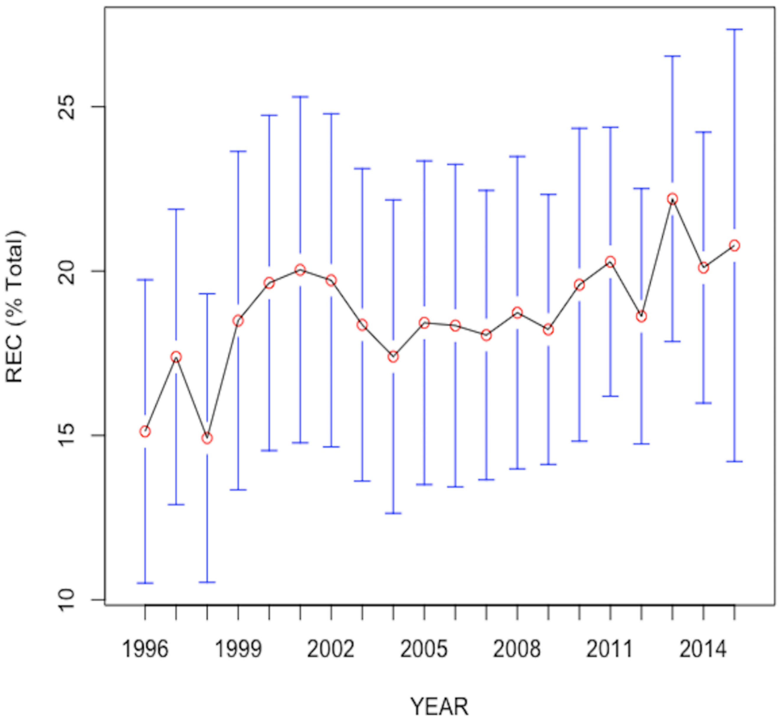
Figure 2 gives a graphical inspection of the evolution of mean renewable energy consumption at world level over the analysis period. Over the past decades, the share of renewable energy consumption in total energy consumption has grown globally from an average annual rate of 15% to 21%, reaching 29% by 2020 [37].

The individual countries’ situation when it comes to renewable energy consumption is both very interesting, and has important policy implications. Appendix D reflects top 20 countries in terms of renewable energy consumption as a percentage of total energy consumption in the most recent year of data availability (i.e., year might differ by country). With the only exception of Iceland, all top five countries with the highest percentage of green energy in their energy mix are low-income countries, with a GDP per capital below 1000 USD (i.e., Ethiopia, Mozambique, Kenya, and Sudan).

The most recent observations in our panel for the two world top polluters China and US show that renewable energy accounted for about 15% of total primary energy consumption in US, whereas 12% of the China’s electricity was sourced from low-carbon sources. However, both countries have increased their relative green energy consumption in recent years and thus move towards attaining their assumed pollution reduction targets (https://ourworldindata.org/energy/country/, accessed on 25 June 2021).

Returning to data in Appendix D, we notice that, with a share of 93% of Ethiopia’s energy consumption, renewable sources (especially waste and biomass (https://energypedia.info/wiki/Ethiopia_Energy_Situation, accessed on 25 June 2021) are the country’s primary energy sources. For Mozambique, renewable energy has a share of 91.3% in total energy consumption, with solar and hydro being the country’s primary energy sources.

When it comes to high and very high-income countries and their endeavor of achieving sustainable development, Iceland, Norway and Sweden are prominent success stories. Iceland, a high-income country, consumed green energy in a percentage of 77% in the most recent year in our data panel for which REC data are available for the country (i.e., 2016) and managed to accomplish a 100% reliance on renewable energy as of the present moment. The main sources of renewables in Iceland are large hydro (75%), and geothermal 25% (https://www.government.is/topics/business-and-industry/energy/, accessed on 25 June 2021). The only very high-income countries that managed to successfully shift their energy systems away from fossil fuels towards low-carbon sources are Norway and Sweden. The two countries also share a common green certificate market since 2012 with the target of rising electricity generation from renewables. In Norway 57.8% of gross final consumption of energy was supplied by renewable sources, while for Sweden the share of green energy amounted to 53.2%. As in Iceland’s case, both of these countries have also moved closer to carbon neutrality in the last years. While hydropower is the source of most of the Norway’s energy production, hydropower and bioenergy are the top renewable sources in Sweden. Moreover, Norway has long been a traditional leader in carbon capture and storage (CCS) technology, which is a climate change mitigation technology where CO₂ is captured from power plants and other industrial processes instead of being emitted to the atmosphere [38]. Previous studies have concluded that low-carbon technologies, including CCS, are essential to meeting the Paris climate agreement objectives [39]. Hence, according to [40], Norway is part of the narrow group of mostly very high-income countries (together with Australia, Canada, United Kingdom and the United States) that are leaders in the creation of an enabling environment for the commercial deployment of CCS, while also leading (together with Canada and the United States) in the Global CCS Storage Indicator (CCS-SI), which evaluates each country’s geological storage potential and the maturity of their storage assessments, while also reflecting the progress of CO₂ storage project deployment and large scale CCS facilities. As of 2007, there were four industrial CCS projects in operation, two of which belonging to Norway [41], while as of 2018 a third facility was in advanced planning stage in Norway [40]. It should be also underlined that Norway is the only low-emitter leader in the CCS technology, which reflects that the country recognizes that climate change is a transnational problem than can only be mitigated through propelling innovation for the global good [42].

In addition, it is worth mentioning that Sweden takes the top spot within the European Union for renewable energy consumption, with Latvia the only other EU country to make this top.

4.1.4. An Overview of the Renewable Energy Consumption—Energy Efficiency (Low Carbon Intensity)—Innovation—Economic Affluence Nexus

An important aspect that delineates low-income and high-income countries that have successfully transitioned towards low-carbon sources is the technology involved in the process. While rich countries had the opportunity to develop and deploy new low-emission technology and infrastructure, poor countries, although naturally endowed with renewable energy sources, lack the ability to successfully exploit it.

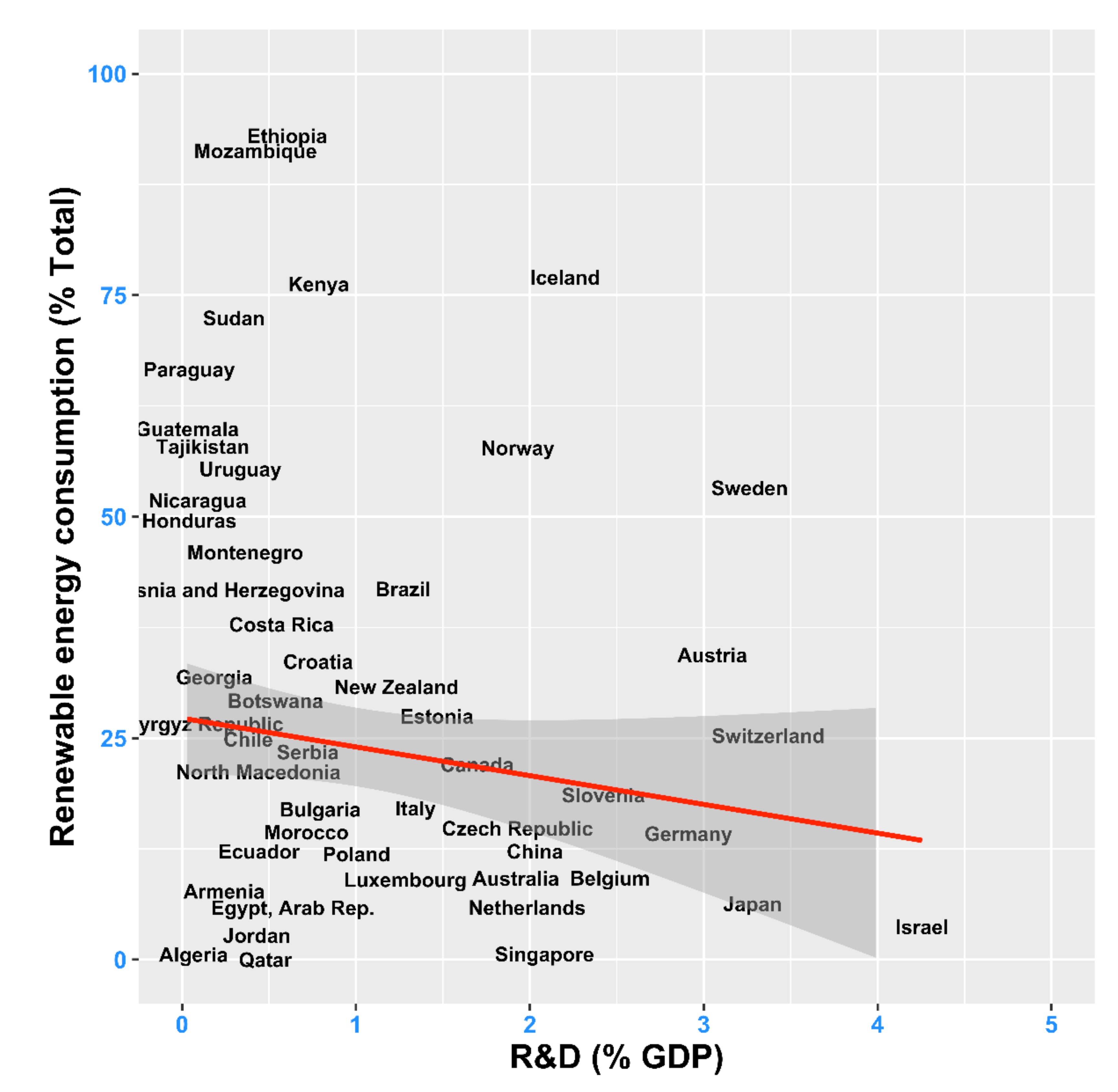
Figure 3 shows all the aforementioned high and very high-income countries that successfully managed to shift their energy mix toward sustainability (Iceland, Norway and Sweden) also undergo large investments in R&D. Other countries that also successfully manage to rip the beneficial effects of R&D investments in terms of increased renewable energy consumption are Luxembourg, Denmark and Switzerland. On the other hand, there are some countries that although prioritize innovation and make investments in research and development, these efforts are not reflected in their energy mix (i.e., Singapore, Korea Rep. or Israel). At the opposing end, countries such as Guatemala, Paraguay and Honduras invest very little in R&D, but nonetheless have an important share of renewables in their energy mix, all due to the availability of renewable energy sources (mostly hydropower, solar and biomass).

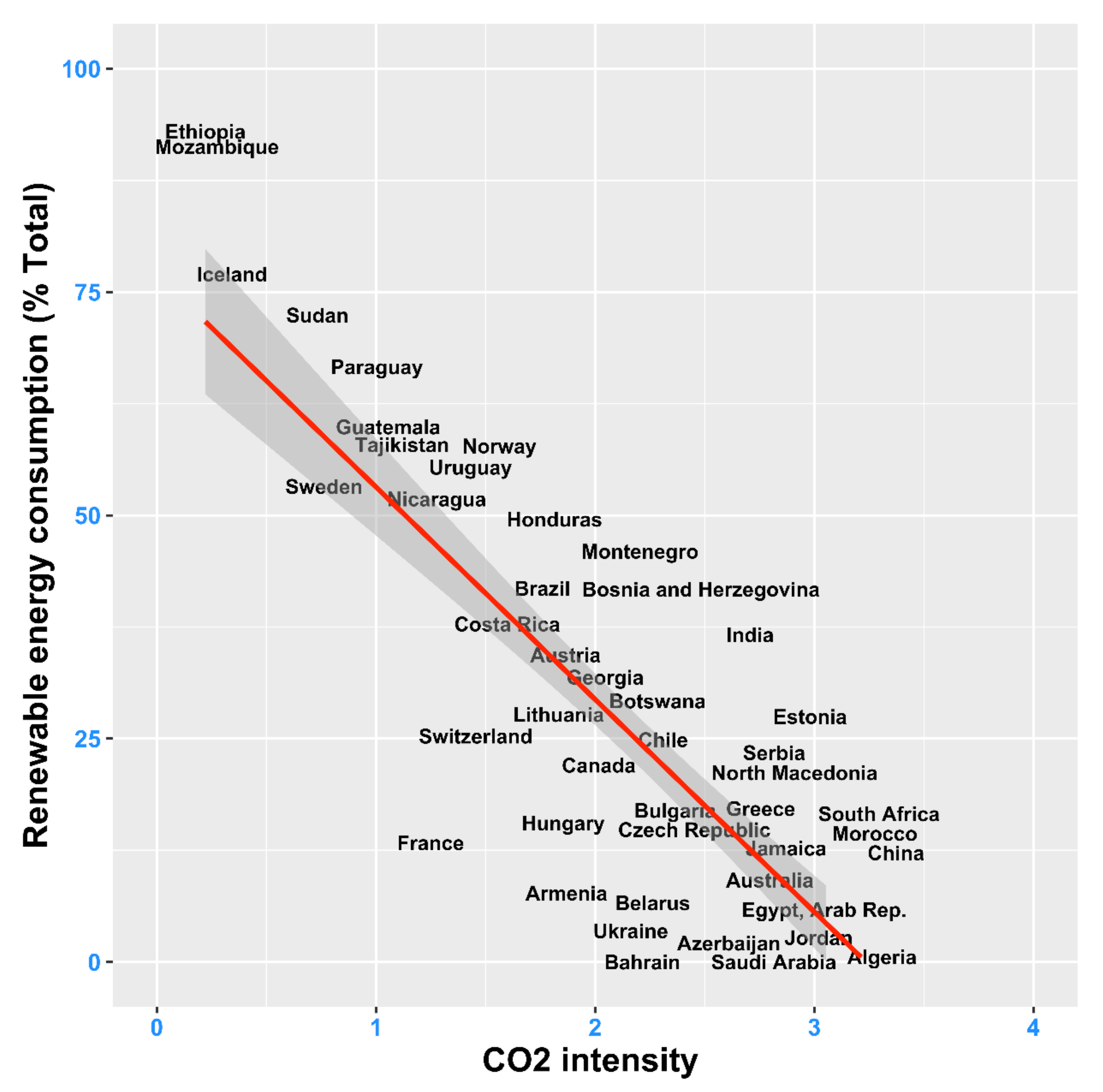
Next, Figure 4 depicts the relationship between the carbon intensity and renewable energy consumption in each country, in the most recent year of available data. The pattern suggests a negative relationship between the CO₂ intensity and REC at world level, which confirms the theoretical insight that increasing energy efficiency (i.e., thereby decreasing CO₂ intensity) results in increased consumption of renewable energy. The countries that present a low level of carbon intensity together with a significant share of renewable energy in their energy mix are Ethiopia, Mozambique and Iceland.

4.2. Estimation Procedures

4.2.1. Preliminary Tests for Model Selection

Figure 5 reflects the means of the dependent variable (REC) by country and attests that there is high heterogeneity across countries, whereas we noticed earlier that the heterogeneity across years is lower (Figure 2).

As such, while the shift towards green energy consumption at world level is apparent over the analyzed period, it is not significantly accentuated, indicating that countries move on average slow in adopting sustainable practices.

In addition, these findings indicate that the basic OLS regression model, which does not consider heterogeneity across countries or across years, is not suitable for our investigations.

This is further confirmed by formally testing for the necessity of including fixed effects in our panel models with an F test for individual effects in the REC equation, which is estimated by comparing the fixed effects model with a pooled OLS model, with the null hypothesis of no fixed effects. Thus, a pooled OLS model estimation has been carried out as well to provide a benchmark model. In the context of this study, the pooled OLS is given by:

$$Y_{it}={\beta }_0+{\beta }_1{X}_{1it}+\dots +{\beta }_4{X}_{4it}+{\epsilon }_{it}+u_i$$

(1)

where $Y_{it}$ is REC in country i and year t, and i is 1,2,3…,n (n = 94) countries, while t is 1,2,3…,t (t = 25) years; $X_{1it}$ to $X_{4it}$ are the four independent variables (i.e., GDP per capita, R&D expenditure, CO2 intensity, and energy use) in country i and year t; ${\epsilon }_{it}$ is the error term of a regression in country i and year t; and $u_i$ are time-invariant factors that impact REC in country i.

The results of the F test (p < 0.01) shows that the null hypothesis of no fixed effects is rejected and attests the presence of country fixed effects.

Next, in order to formally test for the necessity of including random effects in our panel models, we employ the Lagrange multiplier test for random effects, originated from [43], similarly estimated by comparing the random effects model (not shown) with the pooled OLS model. In addition, the null hypothesis is that the variance of the random effect is zero, and one should use Pooled OLS against the alternative hypothesis that the variance of the random effect is larger than zero and should instead use random effects models (REM). The result of the Lagrange multiplier test (p-value = 0.142) confirms that the pooled OLS is preferred to REM, and hence random effects are not present in our data.

Fourthly, to confidently justify our method of choice, we employ the Hausman test [44] to compare the fixed effects (FEM) and the random effects models (REM), where the null hypothesis is that the individual random effects are exogenous and hence REM is suitable (and preferable to FEM). The result of the Hausman test (p < 0.01) indicates that the null hypothesis is rejected, which makes the random effects equation inconsistent.

In conclusion, our preliminary tests all agree that panel models with fixed effects estimators are the correct solution in our future estimations. To assess the effect of model specification on the estimations, dynamic fixed effects models that include lagged dependent variables will also be estimated in the following section, while adjustments for standard errors will be accomplished through robust procedures.

Further, in order to assure that unreliable and spurious regressions are avoided [45,46] we investigate the unit root properties of our data. Stationarity is generally less of a problem in panel data as compared to time series, and testing it usually becomes more important when the number of cross-sections is small and the time series dimension large [47,48]. Although this is not the case with our data panel, where N = 94 (countries) and T = 25 (years), we nonetheless proceed to investigate the stationarity of our data. To this end, the CIPS test for unit root in heterogeneous panels developed by [49] has been estimated. The CIPS panel unit-root test is a second-generation unit root-test that accounts for the dependence that may exist across the different units in the panel, whereas first-generation tests such as the LLC test [50], IPS test [51], MW test [52] and Choi test [53] are based on the (unrealistic) assumption of cross-section independence (see [54] for more details). In this study, as N = 94, the homogeneity assumption is overly restrictive, and as such a second-generation test is required. Results presented in

Table 2. Results of CIPS unit root tests.

Variable	CIPS Unit Root Test
GDP	−3.7582 ***
R&D Expenditure	−3.9974 ***
Energy Use	−4.0731 ***
CO2 Intensity	−4.2484 ***
REC	−4.9534 ***

*** Indicates significance at 1% level.

show that for all the variables in levels the null hypothesis of unit root is rejected as evidenced by small p-values (i.e., p < 0.01) for all series. This implies that the series are stationary in their levels or integrated of order zero, l(0) and hence we can proceed with the estimation of panel fixed effects models at the level. Nonetheless, as [55] explains, it is difficult to interpret the outcome of a panel unit root test if the null of the unit root is rejected. As such, in the case of heterogeneous panel data models with N large and T relatively small (as the current situation), it is only possible to devise sufficiently powerful unit root tests that are informative in some average sense, namely, to inform whether the null of a unit root can be rejected in the case of a significant fraction of the panel members (i.e., countries). Hence, here, the rejection of the panel unit root hypothesis should be interpreted as proof that a substantial proportion of the units are stationary, and not that all the units are stationary. Nonetheless, strictly for the scope of this analysis (i.e., model calibration) the panel unit root test outcome is still valid [55], although it should be employed with caution when it comes to extracting policy implications.

4.2.2. The Fixed Effects (FE) Panel Models

Our relationship of interest, which is further investigated through various panel fixed effects models, is as follows:

REC ~ GDP per capita + CO₂ Intensity+ R&D Expenditure + Energy Use

(2)

The fixed effects model, previously proved to be best suitable for our data sample, takes into account individual differences, translated into different intercepts of the regression line for different individuals (countries). The general (theoretical) form of the model in this case is reflected in Equation (3), where the constant terms calculated in this way are called fixed effects.

$$Y_{it}=({\beta }_0+{\lambda }_i)+{\beta }_1{X}_{1it}+\dots +{\beta }_4{X}_{4it}+{\epsilon }_{it}$$

(3)

where ${\epsilon }_{it}\sim N(o,{\sigma }_u^2)$.

In this investigation, we have a panel regression model with fixed effects estimator for 94 countries i = 1, …, 28, observed at several time periods t = 1, …, 25, where $Y_{it}$ is REC in country i and year t, while the four independent variables employed in the equation will be the income per capita (GDP per capita), R&D expenditure, CO2 intensity and total energy utilization (energy use) in country i and year t, and λ_i is the country specific effect. The ${\epsilon }_{it}$ is the error term that captures the variation in REC that is not explained by the four independent variables $X_{1it}$ to $X_{4it}$, and i is 1,2,3…,n (n = 94) countries, while t is 1,2,3…,t (t = 25) years.

We alternatively estimate a one-way country (or individual) fixed effects model (CFEM) that allows us to detect country-specific effects, which are constant throughout the estimation period, a one-way time fixed effects model (TFEM) that enables us to detect any effects that vary across time but are constant across countries, and a two-way fixed effects model (TWFEM) that controls for both country and time fixed effects.

Next, in order to address common issues within the fixed effects panel models, namely heteroscedasticity, autocorrelation, and cross-sectional dependence, we employ a commonly used robust standard errors computational technique, namely the fixed effects estimator with Driscoll–Kraay standard errors. The research in [56] builds on results from [57] and employs averages of the product between independent factors and model residuals, which are further included in a weighted HAC estimator. Standard errors produced by the Driscoll–Kraay method are robust against autocorrelation, heteroscedasticity, and cross-sectional dependence. Hence, we choose this method to using the Arellano-Bond general method of moments (GMM) estimator [58], which would also give robust standard errors corrected against heteroscedasticity, but which fails to also correct against autocorrelation and cross-sectional dependence, both issues being also present in the data.

We use also lags of the dependent variable REC as instruments following [59,60]. However, we must assess the well-known bias/efficiency trade-off in finite samples when it comes down to a choice of the number (p) of instruments. On the one hand using all the available lags of the instrument variable (p = t) could lower efficiency while on the other hand, reducing the lags to 1 (p = 1) may avoid an over-fit of instrumented variables that might lead to biased coefficient estimates. Based on results from [60], which shows that the choice of instruments does not affect the results, we continue our analysis by adding one lag of the instrument variable, i.e., (p = 1), hereafter specified as REC(−1).

Robustness checks are ultimately conducted to decide on the best-fitting and optimal model specifications for each panel and sub-panel of data.

5. Estimation Results

5.1. Fixed Effects Estimator Results: One-Way Country Fixed Effects (CFEM) Models with Standard Errors

The results of intermediary estimations will be reported throughout the paper, though more focus will be given to robust, error corrected results. Moreover, as the empirical analysis is undertaken for six different panels of countries, accurate estimations of coefficients are obtained.

The results of the individual fixed-effects regression analysis are reported in

Table 3. One-way country fixed effects (CFEM) with standard errors panel model results.

	Total (All 94 Countries)	Low	Middle–Low	Middle–High	High	Very High
	Estimate
GDP	0.0002 ***	(0.0070) *	−0.0003	0.00056781 (***)	0.0001	0.0001
R&D Expenditure	0.5633	(4.8547)	(6.7834) ***	1.2849	2.5976 ***	2.2596 *
CO2 intensity	(5.3704) ***	(14.0131) ***	(3.6364) **	(11.33) ***	(4.3548) **	(15.1351) ***
Energy Use	(0.0001)	(0.006)	(0.0056) ***	−0.0048	0.0011 ***	(0.0022) ***
R-Squared:	0.2122	0.7994	0.3555	0.4043	0.3817	0.8372
Adj.R-Squared:	0.1436	0.7376	0.2485	0.3356	0.3275	0.8058
F-statistic:	75.0989 ***	38.8438 ***	32.4124 ***	57.357 ***	58.789 ***	98.8685 ***
Lagrange Multiplier Test—(Honda)—(for individual effects)	84.637***	3.1852 ***	34.633 ***	41.886 ***	49.432 ***	19.088 ***
Breusch–Godfrey/Wooldridge test (for serial correlation)	485.84 ***	0.31719	83.695 ***	97.317 ***	0.15324	26.135 ***
Pesaran CD test (for cross-sectional dependence)	8.8014 ***	0.82184	1.103	1.2109	1.7476	1.1403

* Indicates significance at 10% level, respectively. ** Indicates significance at 5% level, respectively. *** Indicates significance at 1% level, respectively.

. As seen from data in Table 3, the coefficient for CO₂ intensity is strong, negative and significant at 1% in all sub-samples and also worldwide, with the highest negative impact in both very high income and low-income countries. According to these findings, the CO₂ intensity is the main factor that negatively impacts the consumption of renewable energy at world level. Hence, policies directed towards spurring renewable energy consumption should focus on reducing the CO₂ intensity and thereby increasing energy efficiency.

Innovation (R&D expenditure) is significant only in middle–low, high and very high-income countries. In addition, the coefficient of the economic size is positive and significant only in the country groups that do not have a significant coefficient on R&D expenditure. This might suggest that countries that do not have effective R&D sectors make use of the know-how of other countries to increase their innovation. This is especially valid for middle–high income countries that most probably benefit from knowledge spillovers from the more developed economies. Interestingly, the energy utilization coefficient is significant in all panels where the R&D investments are also significant (i.e., in middle–low, high and very high-income countries), suggesting that these countries direct their innovating efforts towards the development of low-carbon technologies that contribute to increased renewable energy consumption. Surprisingly, the middle–high income countries do not follow this pattern, suggesting that after some initial efforts towards R&D investments, middle–low economies, probably responding to cost pressures, return to cheaper fuel-based energy consumption before reprising their previous efforts towards developing energy-efficient technologies and spurring renewable energy consumption. Economic affluence (GDP per capita) has a positive impact on REC at a global level, and also for the middle high-income countries, confirming that countries do not incur economic costs in their effort to change their energy mix away from unsustainable, cheaper energy sources.

The Lagrange multiplier test (Honda) for individual effects confirms that our panel data contain heterogeneity between countries and thus one-way CFEM models are suited for explaining the data. On the contrary, the Lagrange multiplier test indicates that one-way time fixed effects models (TFEM) are not able to capture the inter-connections between our data. As such, we chose not to report the estimation results for one-way TFEM and proceed to report directly the results from fitting two-way fixed effects models on our unbalanced panels: the whole worldwide panel containing 94 countries and the five sub-panels according to countries’ economic development (

Table 4. Two-way country fixed effects (CFEM) with standard errors panel model results.

	Total (All 94 Countries)	Low	Middle–Low	Middle–High	High	Very High
	Estimate
GDP	0.0002 ***	(0.0234) *	(0.0004)	0.0008 (***)	(0.0004)	0.0004 *
R&D Expenditure	(0.0073)	(7.2485) *	(6.7834) ***	1.3280	(0.1337) ***	3.1171 *
CO2 Intensity	(5.3177) ***	(15.5509) **	(0.8733)	(12.138) ***	(1.4822) ***	(15.8368) ***
Energy Use	0.0000	(0.0051)	(0.0050) **	(0.0054) **	0.0013 ***	(0.0014) *
R-Squared:	0.1666	0.7994	0.3164	0.4043	0.3817	0.8372
Adj.R-Squared:	0.0078	0.7376	0.1340	0.3356	0.3275	0.8058
F-statistic:	54.7805 ***	6.5884 ***	25.1418 ***	48.4724 ***	45.1742 ***	39.8177 ***
Lagrange Multiplier Test—(Honda)—(for individual effects)	58.939 ***	0.6999	22.956 ***	28.186 ***	34.746 ***	12.378 ***
Breusch-Godfrey/Wooldridge test (for serial correlation)	461.61 ***	0.0667	78.458 ***	91.805 ***	17.243 ***	22.953 ***
Pesaran CD test (for cross-sectional dependence)	0.1685	2.8465 **	1.6030	2.055 **	2.683 **	2.2042 **

* Indicates significance at 10% level, respectively. ** Indicates significance at 5% level, respectively. *** Indicates significance at 1% level, respectively.

).

5.2. Fixed Effects Estimator Results: Two-Way Fixed Effects Models with Standard Errors

Table 4 reports the results of two-way fixed effects models estimated on the entire panel of 94 countries and on the five sub-panels corresponding to different income levels.

As can be seen, the results on the relationship between CO₂ intensity and renewable energy consumption are very similar to the ones obtained in the one-way (country) fixed effects analysis. That is, increasing energy efficiency (reducing CO₂ intensity) results in a substantially increased consumption of renewable energy for all country categories. Only the middle–high and very high-income countries have a significant coefficient for economic development (GDP per capita), validating the previous results and suggesting that, after countries make some initial efforts toward carbon-neutrality, they return to unsustainable consumption practices before reaching a turning point in their economic affluence from where the ability of preference towards green energy is triggered. According to our classification, this trigger point in countries’ economic growth seems to lie somewhere on the vicinity of 50,000 USD per capita and might imply some behavioral changes that occur in the population of countries that reach this level of affluence.

5.3. Robustness Checks

However, before proceeding with further discussions of results, their robustness must be checked. As such, we present in

Table 5. Robustness checks for the one-way country panel models with fixed effects estimator and standard errors.

Breusch–Godfrey/Wooldridge test (for serial correlation)	485.84 ***	0.31719	83.695 ***	97.317 ***	0.15324	26.135 ***
Pesaran CD test (for cross-sectional dependence)	8.8014 ***	0.82184	1.103	1.2109	1.7476	1.1403

* Indicates significance at 10% level, respectively. ** Indicates significance at 5% level, respectively. *** Indicates significance at 1% level, respectively.

results of estimations of the Breusch–Godfrey test, which tells us that generally our models do indeed suffer from auto-correlated standard errors. This is not surprising, as serial correlation is common in multi-country series of macroeconomic variables due to dependence arising from global shocks and other more complex interdependencies [61]. Accordingly, we know that we need to adjust the standard errors, which will be accomplished in the following subsection. In addition, the Pesaran cross-sectional dependence test presented in

Table 6. Robustness checks for the two-way panel models with fixed effects estimator and standard errors.

Breusch–Godfrey/Wooldridge test (for serial correlation)	461.61 ***	0.0667	78.458 ***	91.805 ***	172.43 ***	22.953 ***
Pesaran CD test (for cross-sectional dependence)	0.1685	2.8465 **	1.6030	2.055 **	2.683 **	2.2042 **

* Indicates significance at 10% level, respectively. ** Indicates significance at 5% level, respectively. *** Indicates significance at 1% level, respectively.

confirms the presence of cross-sectional dependence in most of our models. Thus, this will also be further adjusted via robust procedures.

5.4. Robust Dynamic Panel Models with a Fixed Effects Estimator and Driscoll–Kraay Standard Errors

In order to address previous encountered issues with data, we further estimate dynamic panel models with fixed effects, which include a lagged dependent variable (LDV), with the Driscoll and Kraay’s method that produces heteroskedasticity and autocorrelation consistent errors that are robust to cross-sectional dependence.

Table 7. Estimation results of dynamic panel models with a fixed effects estimator and robust Driscoll–Kraay standard errors (one-way CFEM and two-way FE).

	Total (All 94 Countries)	Low	Middle–Low	Middle–High	High	Very High
PANEL A: dynamic one-way country fixed effects model
REC(-1)	0.8600 ***	(0.0241)	0.7193 ***	0.7256 ***	0.9105 ***	0.8600 ***
GDP	0.0000	(0.0040)	0.0001	0.0002 *	0.0001 *	0.0001 *
Expenditure	0.3181	(15.8540)	(1.3133)	0.8275	0.3937	3.1171 *
CO2 Intensity	(1.9818) ***	(17.7137) ***	(0.8245)	(4.8236) ***	(1.4822) ***	(6.8213) ***
Use	(0.0002)	(0.0051)	(0.0031) **	(0.0019) **	0.0000	(0.0007) ***
R-Squared:	0.7906	0.7948	0.7108	0.7600	0.8652	0.9618
Adj.R-Squared:	0.7701	0.7208	0.6576	0.7273	0.8251	0.9586
F-statistic:	694.942 ***	19.365 ***	85.5434 ***	175.418 ***	413.472 ***	271.957 ***
PANEL B: dynamic two-way fixed effects models
	Total (All 94 Countries)	Low	Middle–Low	Middle–High	High	Very High
	Estimate
REC(-1)	0.8553 ***	0.0187	0.7253 ***	0.7214 ***	0.7938 ***	0.7487 ***
GDP	0.0000	(0.0408)	0.0002	0.0000	(0.0001) **	0.0001 *
R&D Expenditure	0.1784	(9.6408)	(2.0104)	0.5715	(0.0451)	3.1790
CO2 Intensity	(1.9780) ***	(7.8123) **	(4.3718) ***	(4.3111) ***	(0.6878) ***	(6.1672) ***
Energy Use	(0.0002)	(0.0001)	(0.0026)	(0.0021) **	0.0002 *	(0.0004)
R-Squared:	0.7609	0.4863	0.7062	0.7256	0.7297	0.9273
Adj.R-Squared:	0.7133	0.2218	0.6156	0.6662	0.6870	0.8751
F-statistic:	694.942 ***	19.365 ***	855.434 ***	175.418 ***	413.472 ***	271.957 ***

* Indicates significance at 10% level, respectively. ** Indicates significance at 5% level, respectively. *** Indicates significance at 1% level, respectively.

presents the estimation results of the dynamic one-way country fixed effects regression with Driscoll–Kraay standard errors for the five categories of countries and also for the overall panel (Panel A), while the estimation results of the dynamic two-way fixed effects regression with Driscoll–Kraay standard errors for the same panels/sub-panels are presented in Panel B. Two robustness checks are subsequently conducted for the best-fitting models, i.e., the Breusch–Godfrey/Wooldridge test for investigating if serial correlation is still left in the residuals, and the Pesaran CD test for cross-sectional dependence.

Firstly, we notice that the best-fitting robust model for each panel and sub-panel is the dynamic one-way country fixed effects model (DOWCFEM) with Driscoll–Kraay standard errors. The overall goodness-of-fit is very high (i.e., Adjusted R-squared = 77% for the entire panel of countries, and 95.86% for the very high-income subpanel), showing that most of the variation in renewable energy consumption can be explained by variation in the model’s parameters. That inspires confidence that most big macroeconomic and environmental determinants of REC have been included in the model either directly or indirectly.

In addition, both robustness tests indicate that all six dynamic one-way country fixed effects panel models with Driscoll–Kraay standard errors are well specified, and results are robust (

Table 8. Robustness checks for the dynamic (one-way) panel models with fixed effects estimator and Driscoll–Kraay standard errors.

	Total (All 94 Countries)	Low	Middle–Low	Middle–High	High	Very High
Breusch–Godfrey/Wooldridge test (for serial correlation)	0.2091	0.3133	4.8778	6.8521 *	0.0532	1.1967
Pesaran CD test (for cross-sectional dependence)	1.2649	0.3822	1.6030	1.5724	0.8435	0.8897

* Indicates significance at 10% level, respectively.

). The serial correlation is now captured in these dynamic models and allows us to observe the short-term and long- term effects between the variables of interest.

6. Discussion of Results

The above results indicate that energy efficiency achieved through reducing CO₂ intensity is the main driver for renewable energy consumption at world level, and that low-income and very high-income countries are able to extract the most benefits from this relationship, with statistically significant negative coefficients of (17.7137) for poor countries and (6.8213) for very rich countries. This in turn shows the importance of decreasing carbon intensity for low-income polluters such as India or very high-income CO₂ emitters (i.e., US, Canada). These countries should especially prioritize efforts to reduce carbon intensity at a fast pace. Similar to the conclusion of [62,63], results thus indicate that ambitious policies targeted towards energy efficiency represent a successful strategy that should be exploited worldwide to a much larger extent.

A country can achieve a lower carbon-intensity of fossil-fuel combustion through relying on renewable sources such as hydropower, wind, solar, and biomass. Additionally, technological advances (i.e., development of low-carbon technologies, such as carbon capture and storage (CCS)) also help to reduce the carbon intensity of fossil-fuel combustion [64] and to increase the efficiency in energy use [65]. Other ways for an economy to reduce CO₂ intensity are to source energy from nuclear and to lower the dominance of coal in its energy mix [66]. As [67] shows, three-quarters of the total primary energy supply in low-income countries is renewable biomass. Hence, we can confidently infer that the high negative relationship between CO₂ intensity and renewable energy consumption (slope of −17.7137) for low-income countries is explained by the fact that they generally rely heavily on biomass as a fuel source, (i.e., Ethiopia, the highest placed country in the renewable energy consumption classification in Appendix D sources 92.4% of its energy supply from waste and biomass (Ethiopia Energy Situation, https://energypedia.info/wiki/Ethiopia_Energy_Situation, accessed on 3 September 2021). The negative relationship between CO₂ intensity and renewable energy consumption (slope of −6.8213) for very high-income countries can be explained two-fold, depending on their pollution emitting status. Consequently, for the rich countries that have successfully shift their energy mix towards sustainability (i.e., Denmark, Norway, Sweden, Iceland), their increased reliance on renewables (mostly hydropower) achieved through technological innovation explains the relationship. These findings are in line with those of [68] that show that the Nordic European countries (i.e., Denmark, Norway, Finland and Sweden) are world leaders in energy innovation, which has been achieved, among others, through increasing public energy R&D. On the other hand, for rich top polluters such as Australia, Canada, United Kingdom and the United States, the development and employment of CCS technologies support the relationship. Some very-high income countries such as Norway are common denominators for the two sub-categories within the very-high income panel.

Indeed, this assumption is validated by the fact that an increased innovation through R&D investment is positively related to increased renewable energy consumption (statistically significant slope coefficient of 3.1171) only in the case of very high-income countries. This further suggests that lower income countries are not able to achieve a positive impact of R&D expenditure on REC or that their R&D efforts are not directed towards the development of green technologies. Hence, if their energy efficiency is not achieved through the development of low-carbon technologies, this means it is explained either by reliance on readily available renewable energy sources and/or through knowledge spillover effects form the very-high income innovative economies. The results deviate from the findings of [33], which conclude that research and development is the leading driving factor for renewable energy consumption in middle-income countries from G20. The additional number of countries included in our study could explain this divergence. As such, our findings suggest that public spending on R&D does not yield an automatic return in terms of increasing renewable energy consumption and allowing a country to achieve carbon neutrality. The relationship seems to be not only group-specific, but also country-specific, and as such depend on both income and the national context: while very high-income countries uniformly benefit from their R&D efforts, only some high-income countries that prioritize innovation as reflected in public R&D investments extract benefits in term of increasing dependence on sustainable sources (i.e., Iceland), whereas others do not accomplish this goal in spite of their innovative efforts (i.e., Singapore, Korea Republic, or Israel), which could be explained either by ineffective R&D sectors, ineffective energy policies or by directing their R&D efforts towards other priority areas.

Other findings suggest that the negative effect of energy utilization in middle–low income countries is twice its effect in the middle–high income countries, and five times its effect in the very high-income countries. Our results support those of [69], which show that energy use is a mitigating factor for renewable energy consumption growth in selected African countries. These findings imply that when countries increase their energy utilization, they actually increase their consumption of unsustainable energy, and this is especially valid for middle–low income countries. One potential explanation for these results is that middle–low income economies tend to grow through activities that require large energy inputs (i.e., industry, manufacturing, and construction) and rely strongly on cheaper fossil sources. As economies grow, they increasingly direct their attention toward sustainable development, but our results nonetheless confirm that a complete decoupling between energy utilization and reliance on fossil fuel has not been achieved. Consequently, countries that increase the overall utilization of energy are in fact decreasing consumption of renewable energy, but this relationship is much stronger for middle–low income countries (a category which at one point included top polluters such as China, India and Iran) than for the very high-income countries.

Additional findings show a positive correlation between economic development (GDP per person) and renewable energy consumption, but only for the countries with middle–high, high and very high income levels. This suggests that there is a turning point at around 5000 USD per capita where economies begin to afford more expensive energy sources and are thus able to increase their consumption of green energy. These results are in line of those of [30] that concludes that income is a major driver for renewable energy consumption in the case of G7 countries, and of [31] that confirms the relationship for a sample of 18 emerging economies (which are mostly included in the middle and high categories in the present study).

In addition, a further significant finding shows that the consumption of green energy has a persistent positive impact for all income groups, with the exception of the very poor countries, with a GDP per capita below 1000 USD. This suggests the extrapolating benefits of achieving the ability to consume renewable energy, the need for policies directed towards increasing REC, which prove to be sustainable and also the international support that needs to be directed towards poor countries in order to help them reach energy sustainability.

7. Conclusions

Climate change and climate change actions have been prominent factors on the international agenda over the last decades. The global climate change combat reached a historic point through the commitments assumed by 195 signatory countries within the November 2015 Paris agreement, which was enforced in November 2016. As such, decreasing greenhouse emissions is a common and current global endeavor, and the validated solution is that world economies be able to gradually and consistently increase renewable energy in their energy mix until the point of reaching carbon neutrality. The development of renewable energy is thus the validated factor to tackle climate change and spur low-carbon sustainable development.

As proof that this solution is being implemented at world level stands the fact that renewable energy consumption registered a growth trend over the analysis period, globally increasing from 15% to over 21% of total primary energy consumption. However, our results reflect that the level of green energy in the energy mix of individual countries remains highly heterogenic, suggesting that countries are on a different path in meeting their pollution mitigation commitments. Worldwide, Ethiopia and Mozambique, two low-income countries, have the highest levels of REC (of 93%, and 91.3% respectively), while the high- and very high-income countries that have achieved the highest level of renewable energy consumption are Iceland, Norway and Sweden (with approximately 77%, 57% and 53% respectively). The two world top polluters China and US registered levels for renewable energy consumption that are still below the world average (with 12% in the case of China and 15% for the US), although the share of sustainable energy in their energy mix has been increasing in recent years in both countries.

Although the literature on renewable energy consumption and its driving factors has grown over the last few years, there is no known study that examined the individual and synergic effect of economic development, innovation propensity (R&D expenditure), energy efficiency (proxied by low CO₂ intensity) and total energy utilization, using a broad variety of robust panel models. As such, this study investigated this complex, relevant and current relationships using data from 1995 to 2019 based on a wide panel of 94 developing countries. The best-fitting robust model for all panels/sub-panels is found to be the dynamic panel (one-way) model with fixed effects estimator and Driscoll–Kraay standard errors.

Overall, the results obtained from the analysis of the relationship between REC and carbon intensity, innovation (R&D expenditure), economic development (GDP per capita) and energy utilization allows us to extract the following conclusions and offer the following answers to the stated research questions:

First, there is a positive correlation between income (GDP per person) and renewable energy consumption, but only for the countries with middle–high, high and very high income, suggesting that after they move above 5000 USD per capita economies begin to afford sustainable (but more expensive) energy sources.

Second, a country’s propensity towards innovation (through R&D investment) is positively related to increased renewable energy consumption only in the case of very high-income countries, thus reflecting that only very rich countries seem to be able to make use of their innovation skills towards increasing their dependence on green energy sources and moving towards carbon-neutrality.

Third, the strongest result of the study is that CO₂ intensity is a mitigating factor for renewable energy consumption at world level, but especially for countries in the low-income and very high-income sub-panels. This further implies that world top polluters (both low-income polluters such as India or very high-income CO₂ emitters such as US and Canada) must prioritize policies directed towards decreasing carbon intensity (through investing in low-carbon technologies, among others), which would allow them to successfully change their energy mix towards sustainability.

Forth, as already acknowledged, there is a differential impact of some REC driving factors for different income-groups of countries. Only the CO₂ intensity and total energy utilization have an overall effect on REC that remains consistent, although its intensity varies, across the sub-panels. As such, other results indicate significant different levels of the negative impact of total energy utilization on REC, the negative relationship being the strongest for middle–low income countries, and the weakest for the very high-income countries, further suggesting that, as economies grow, they increasingly direct their attention towards sustainable energy sources and carbon neutrality, although a complete decoupling between energy utilization and reliance on fossil fuel has not been consistently achieved, except for some individual “success stories” such as Iceland, Norway or Sweden.

Important policy implications emerge from the empirical results. Without a doubt, sustainable energy policies are needed to allow countries to meet their assumed targets within the Paris agreement and other international agendas (i.e., The European Green Deal). However, the right policy is relatively different according to country-specific factors, although some generally valid policy directions also emerge. As such, while reducing CO₂ intensity is indeed a general driver of increased green energy consumption and thus of carbon neutrality, there are different ways of achieving it: on one hand, low- and middle-income countries would benefit from knowledge spillovers and transfer of green-technology from more performing innovators; on the other hand, high and very-high income nations should direct their efforts towards investment in innovation and developing low-carbon technology. The employment of post-COVID-19 recovery funds, which are at the forefront of international agendas, towards investments in renewables, constitutes an ideal occasion. Thus, for the policymakers, it is necessary to pay attention to the differential effects of all REC drivers in order to issue effective and targeted energy policies.

Overall, this study argues that if countries prioritize policies to increase renewable energy consumption through reduced CO₂ intensity and hence increased energy efficiency via transfer or development of innovative low-carbon technologies, taking advantage of the recovery funds available in the aftermath of the global pandemic, they will be able to meet international assumed climate combat targets and contribute to tackle the stringent global warming problem, while avoiding economic costs.