
Comparison of Star and String Offshore DC Collector Grid Topologies on the Aspect of Stability—An Impedance Approach

 , , ,
, , ,  and
and 
Abstract
:1. Introduction
- An impedance-based modelling approach for off-shore WT systems, submarine cable and input impedance of three phase DAB;
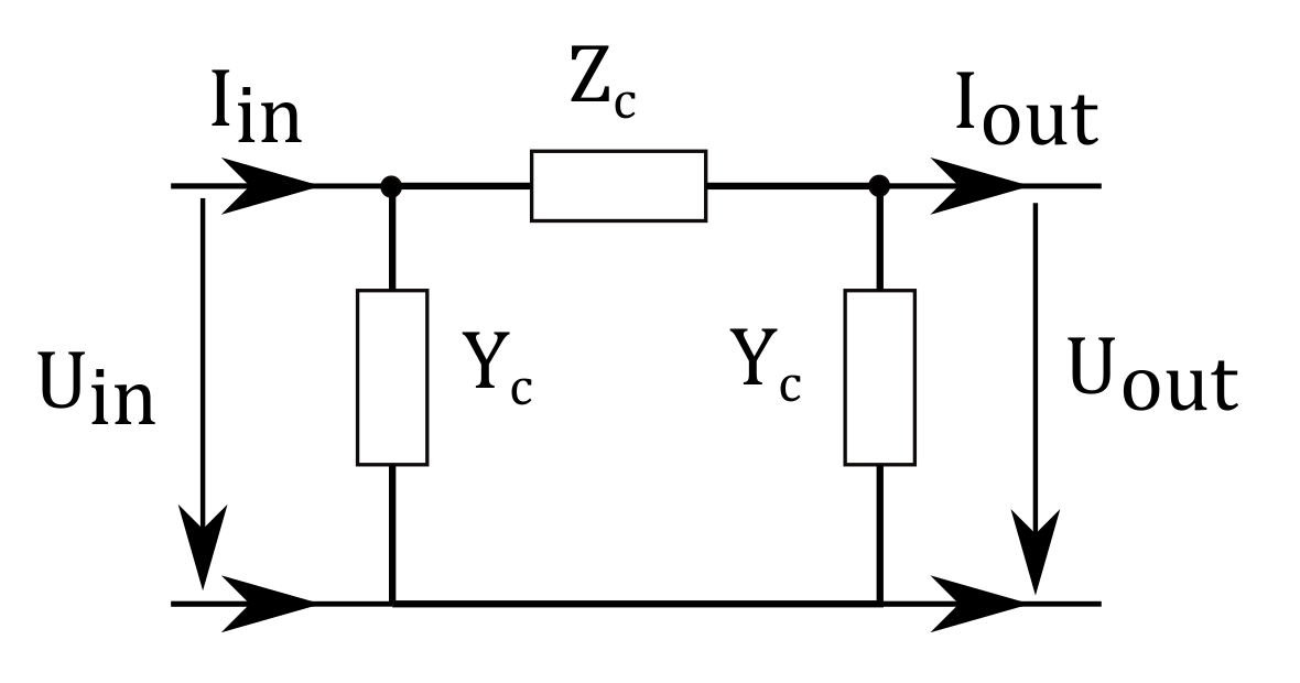
- A non-parametric network impedance building algorithm based on two-port network theory via transmission matrices;
- Application of non-parametric impedance-based stability analysis for offshore DC collector grids;
- An effective comparison between star and string offshore WT typologies on the aspect of system stability.
2. Topologies of Offshore Wind Farms
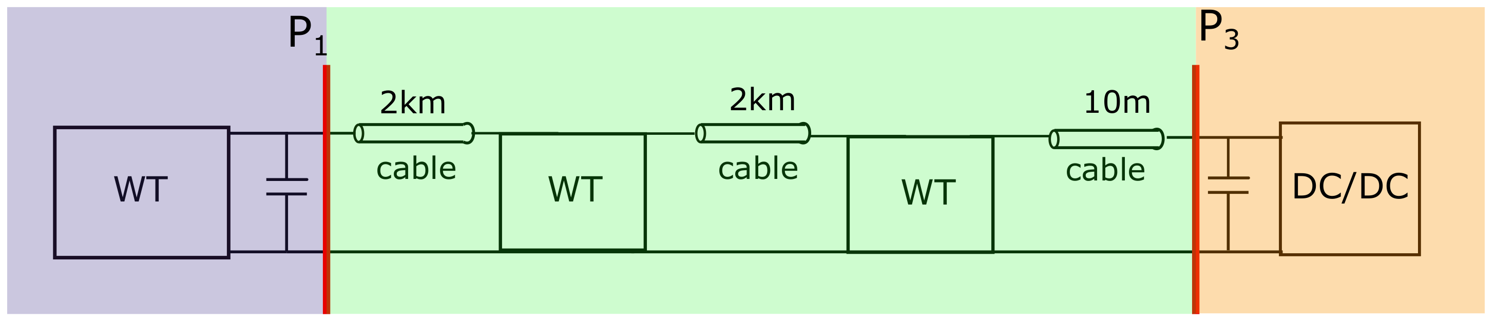
2.1. String
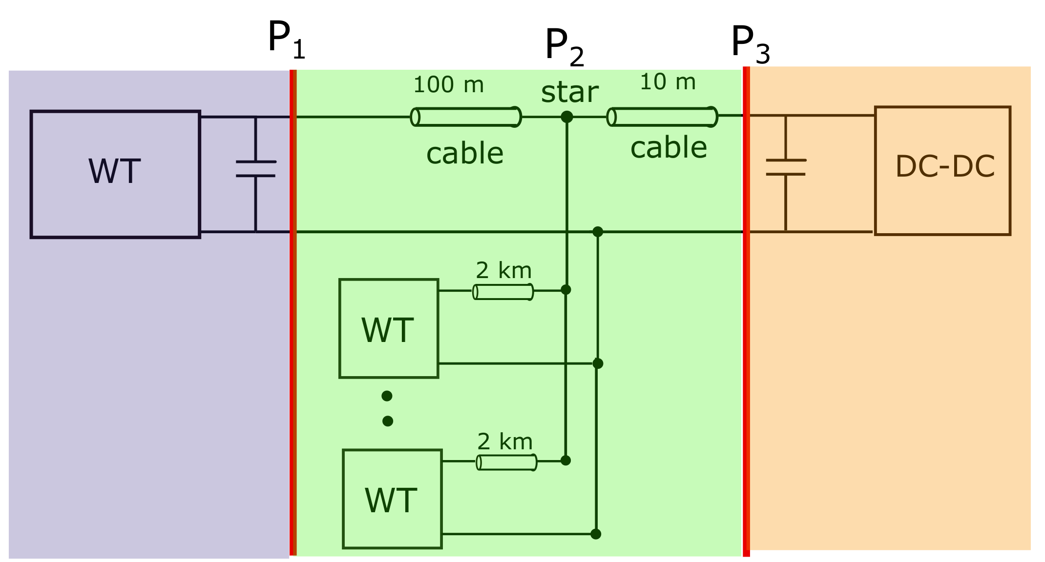
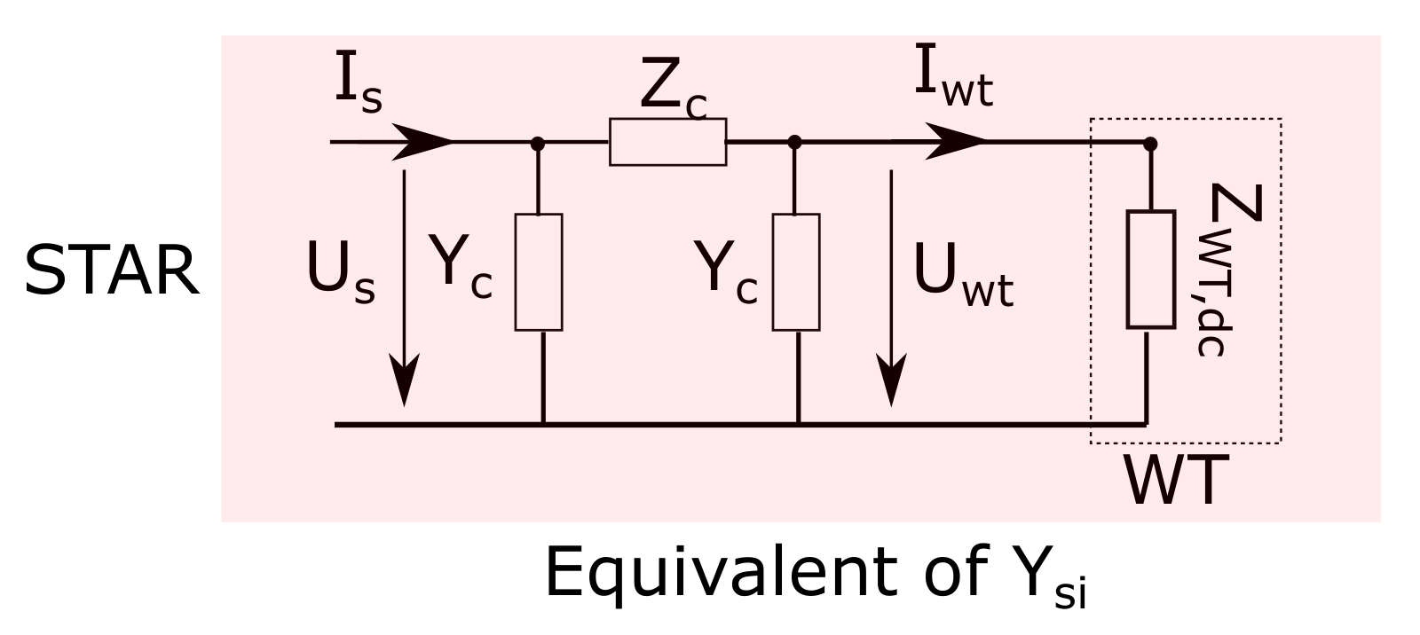
2.2. Star
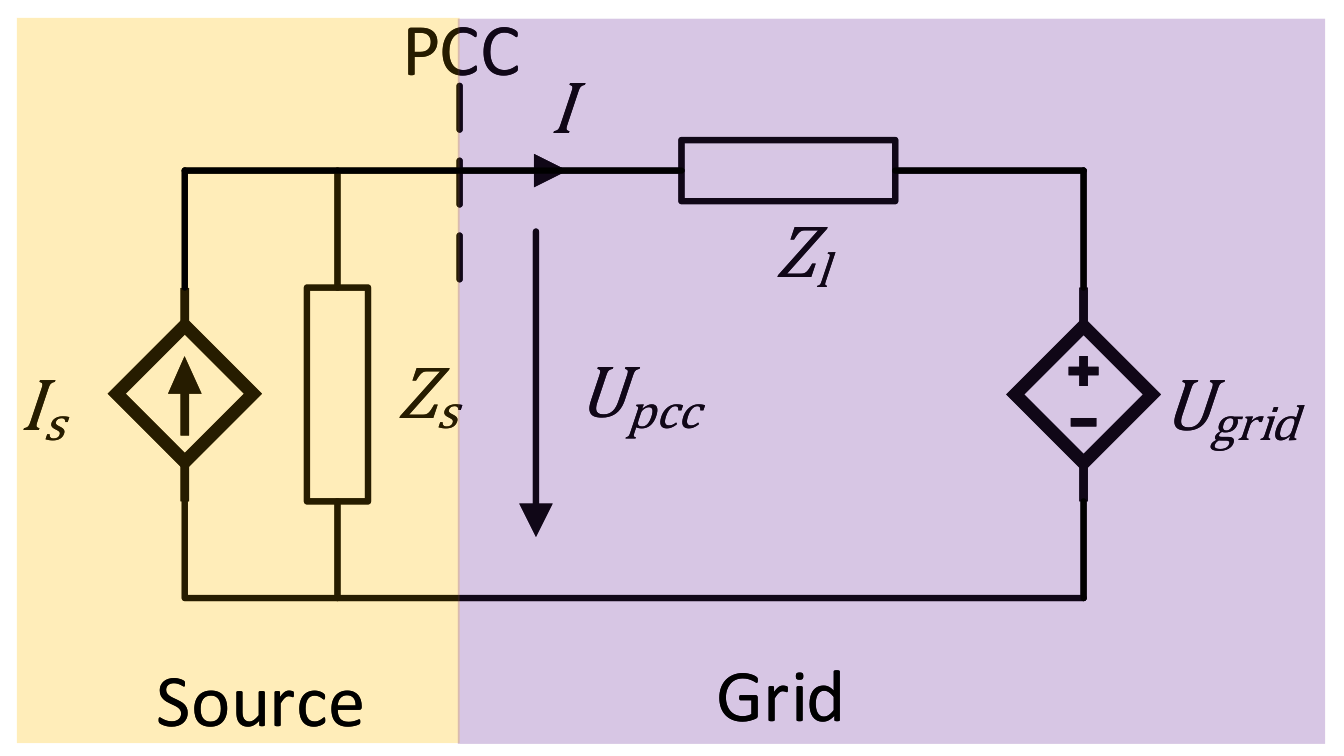
3. Impedance Based Stability Criterion
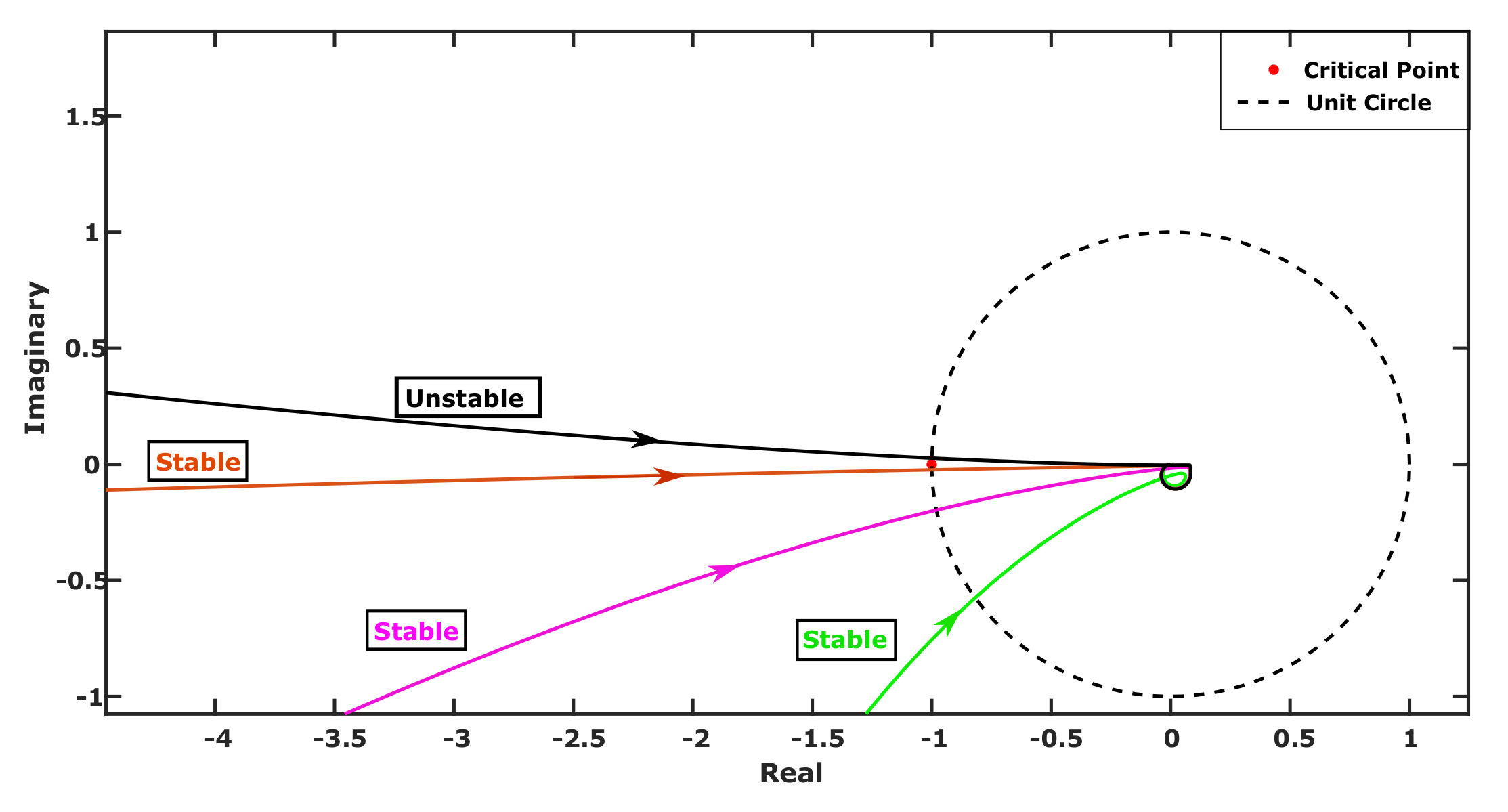
3.1. Nyquist Stability Criterion
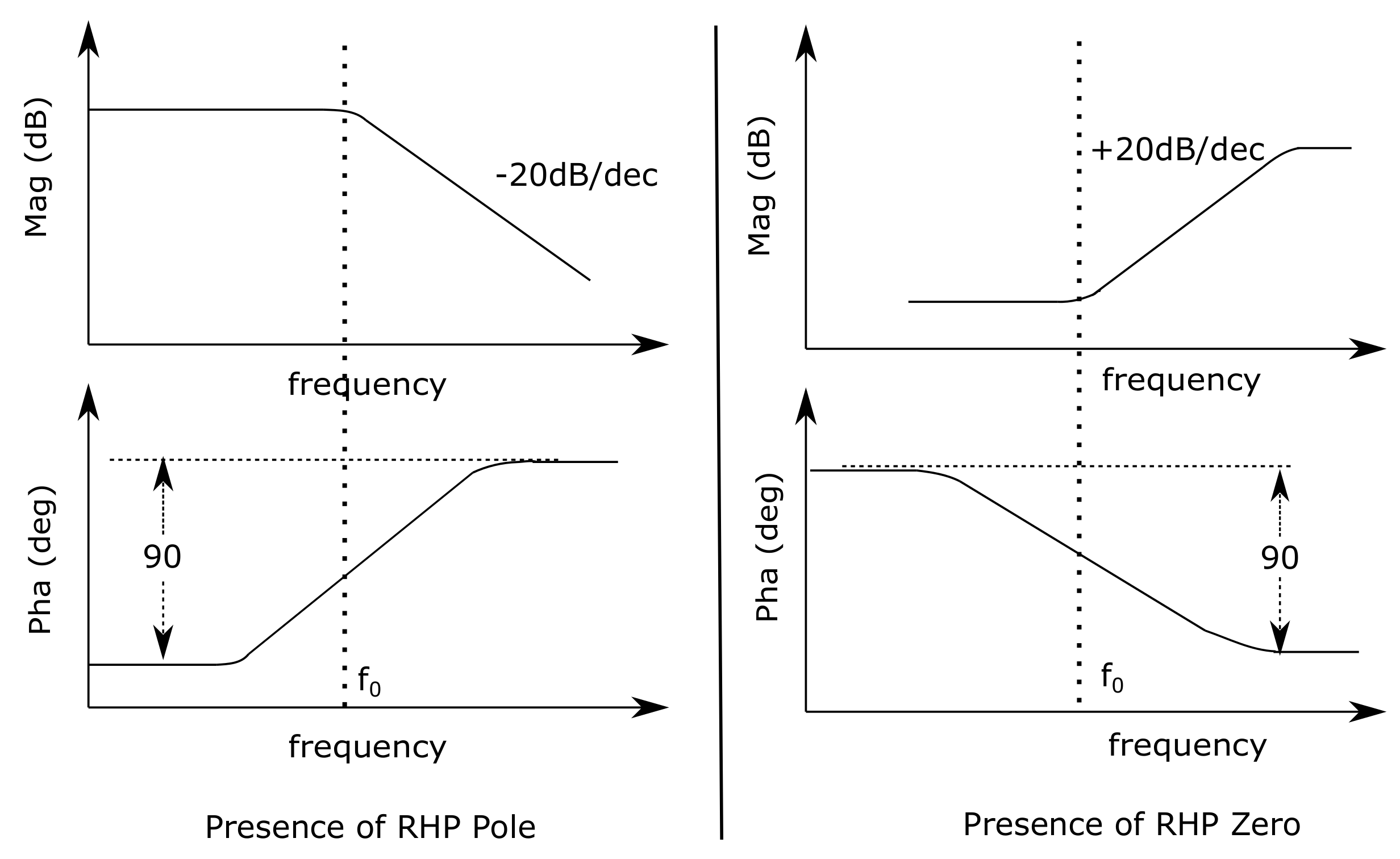
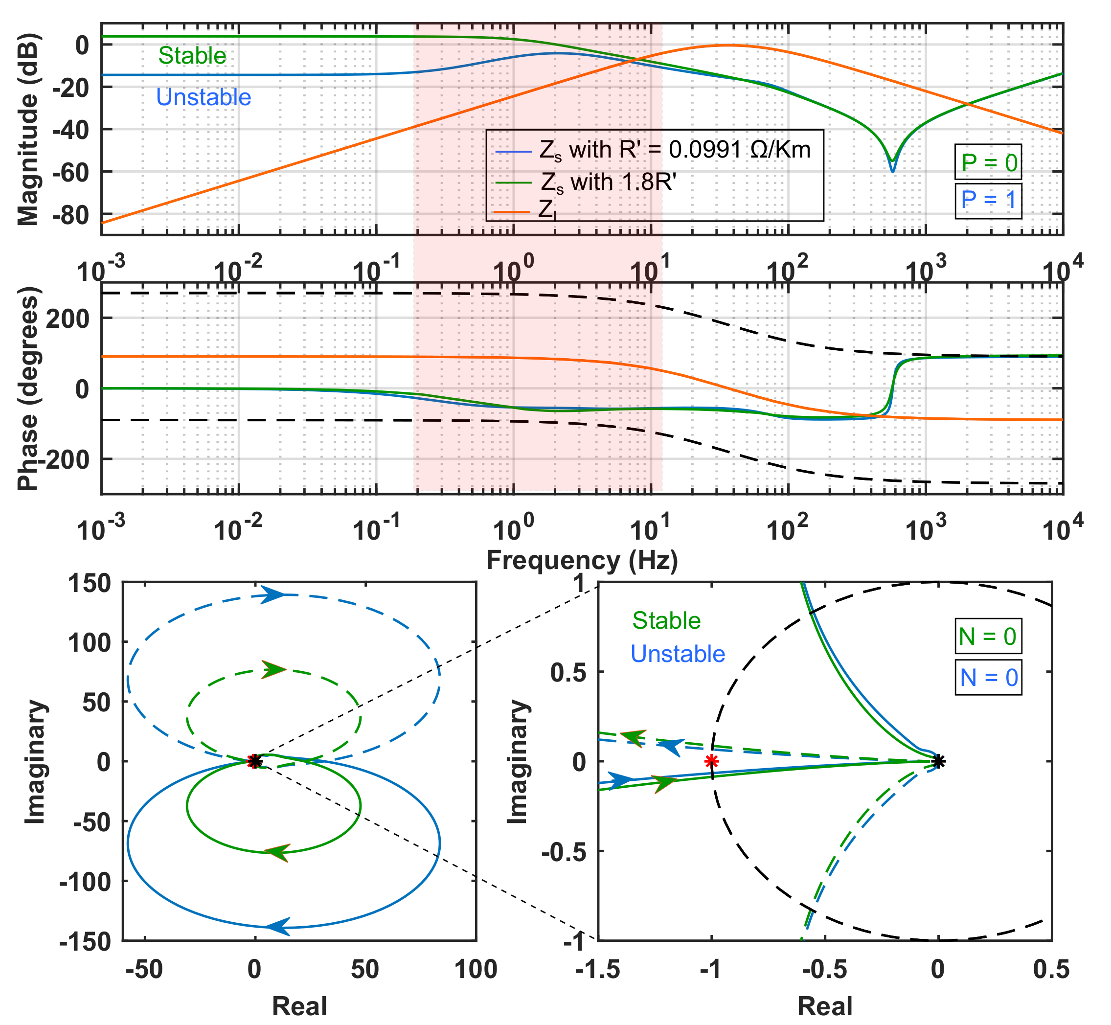
3.2. Non-Parametric Nyquist Stability Criterion
- If the two impedances have different slope magnitudes at high frequency, the numerator impedance should be chosen as the one with smaller slope magnitude;
- If the two impedances have same slope magnitude at a high frequency, the numerator impedance should be chosen as the one with a smaller magnitude at high frequency.
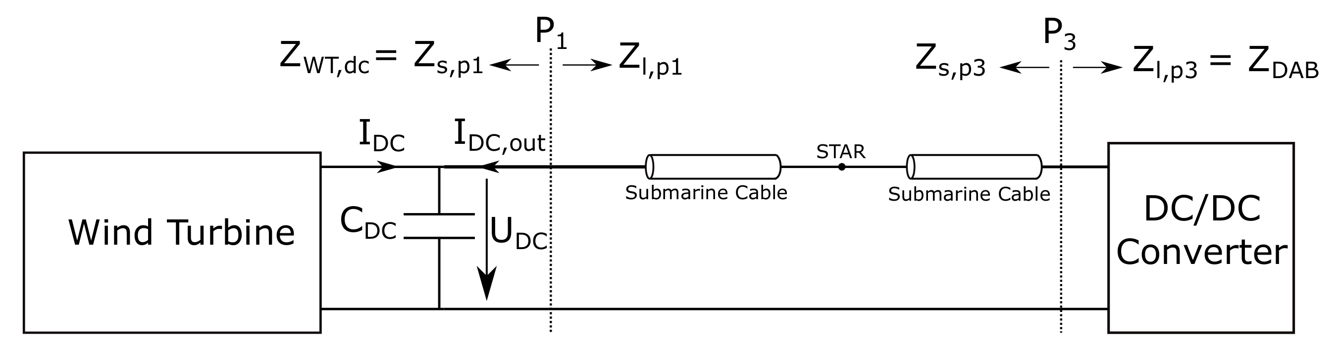
4. Impedance Modelling of the Interconnected System
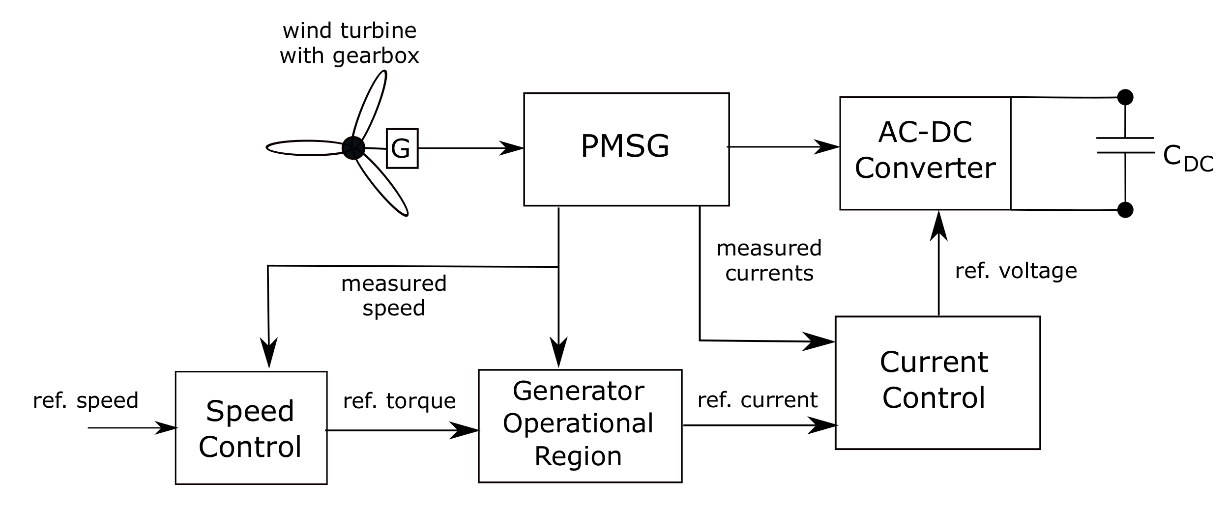
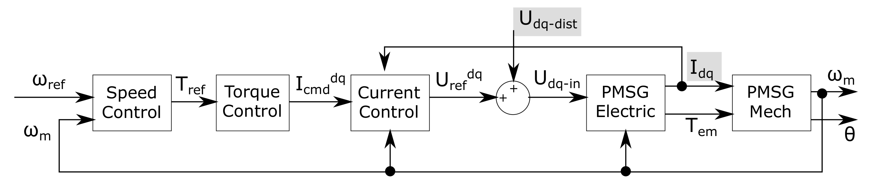
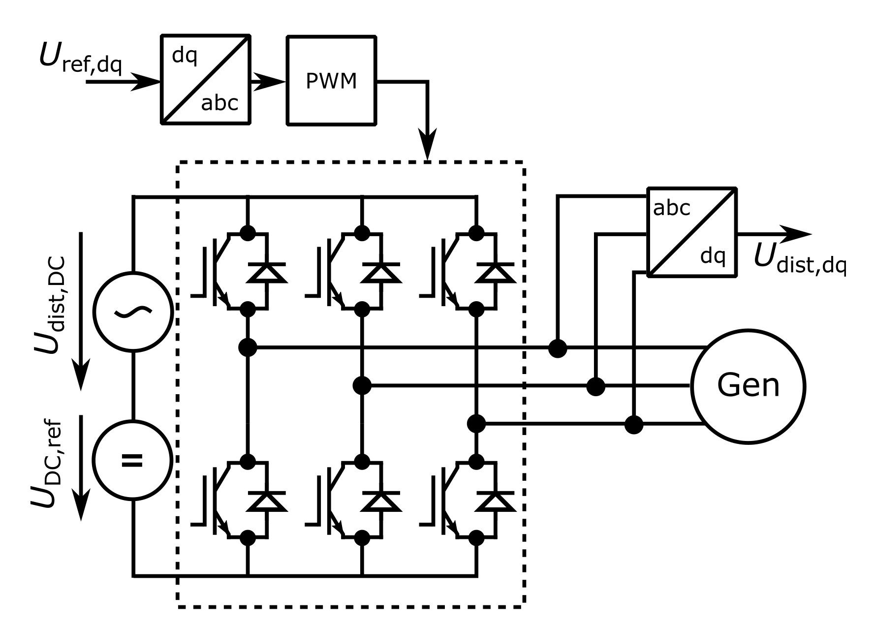
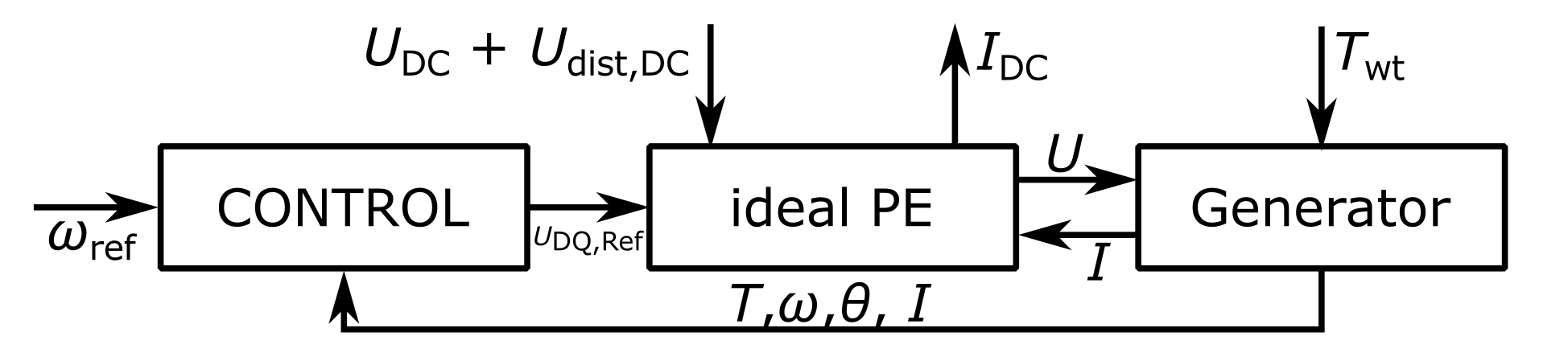
4.1. Model of the Wind Turbine System
4.1.1. PMSG
4.1.2. Speed Control
4.1.3. Generator Operational Region
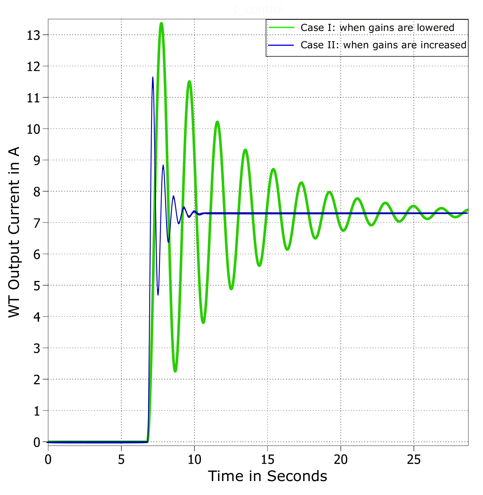
4.1.4. Current Control
4.2. Modelling of Submarine Cables
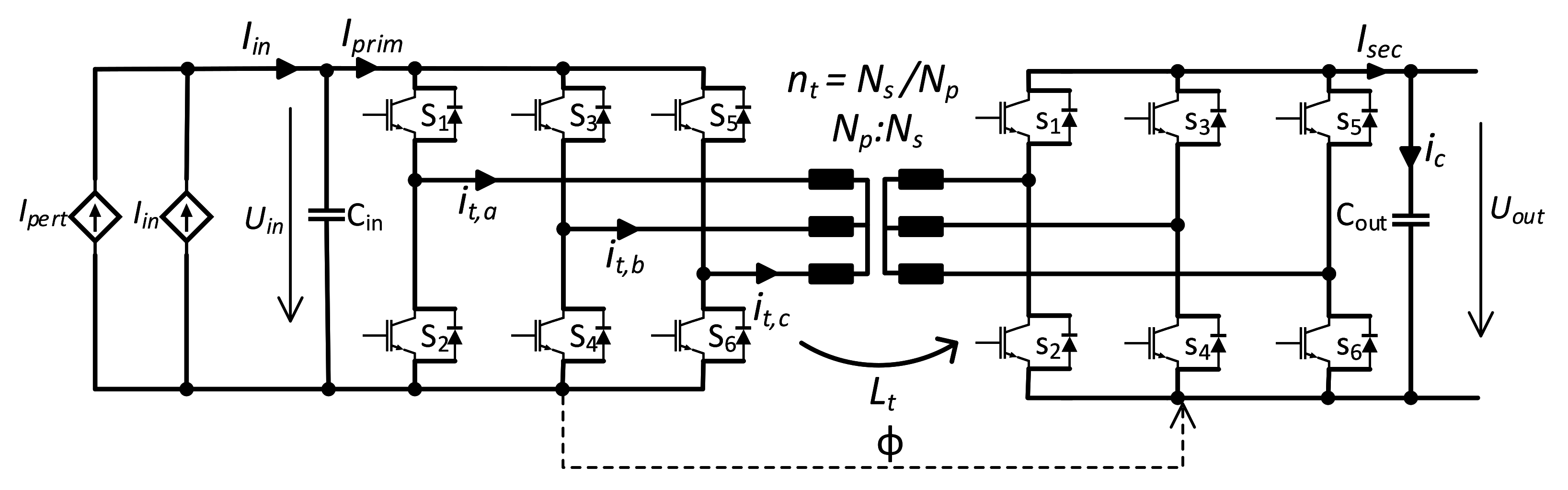
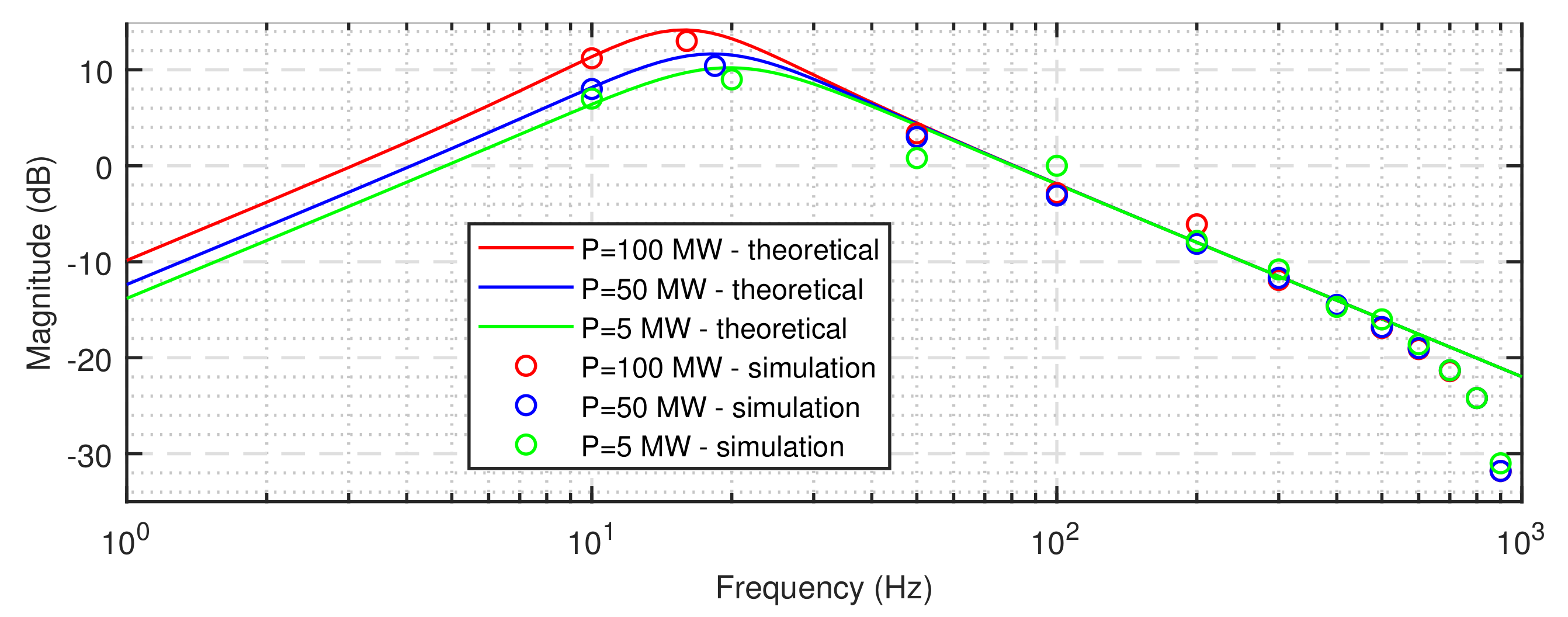
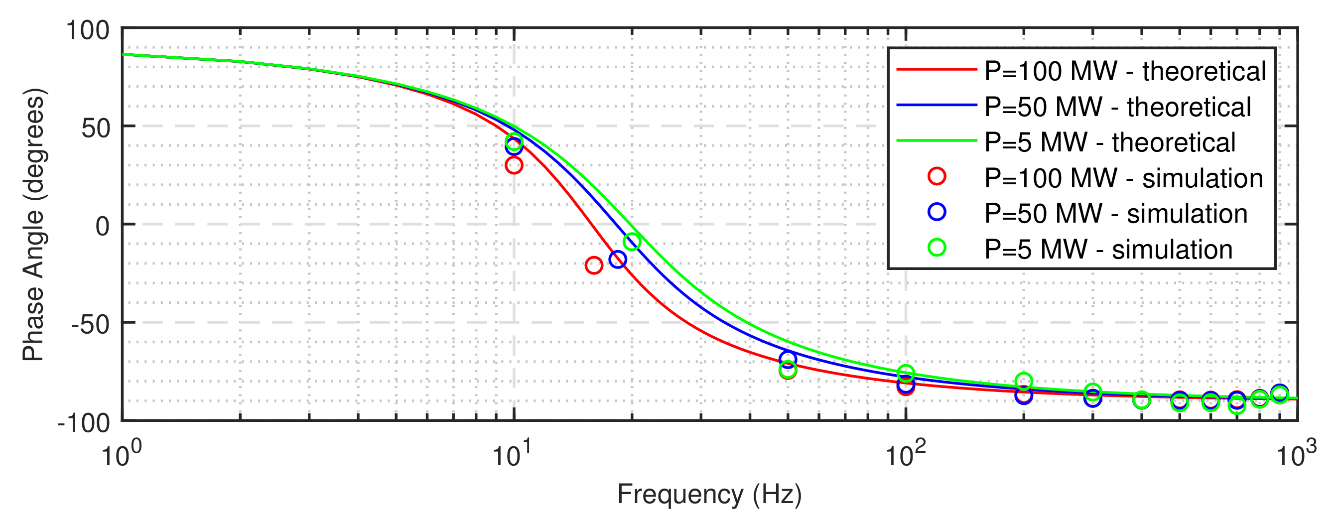
4.3. Modelling of DC/DC Converter
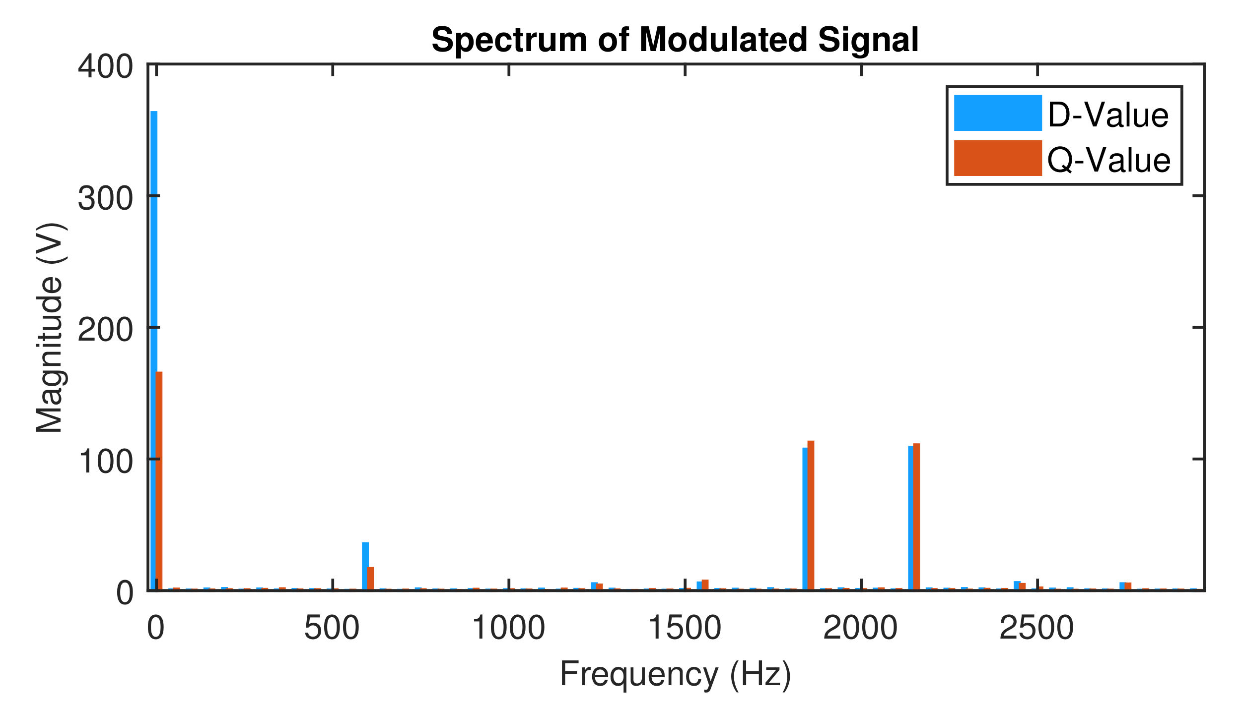
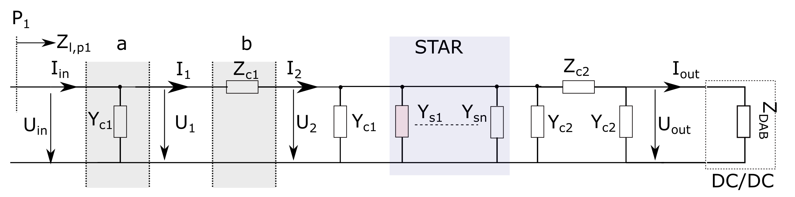
5. Non-Parametric Impedance Building Algorithm
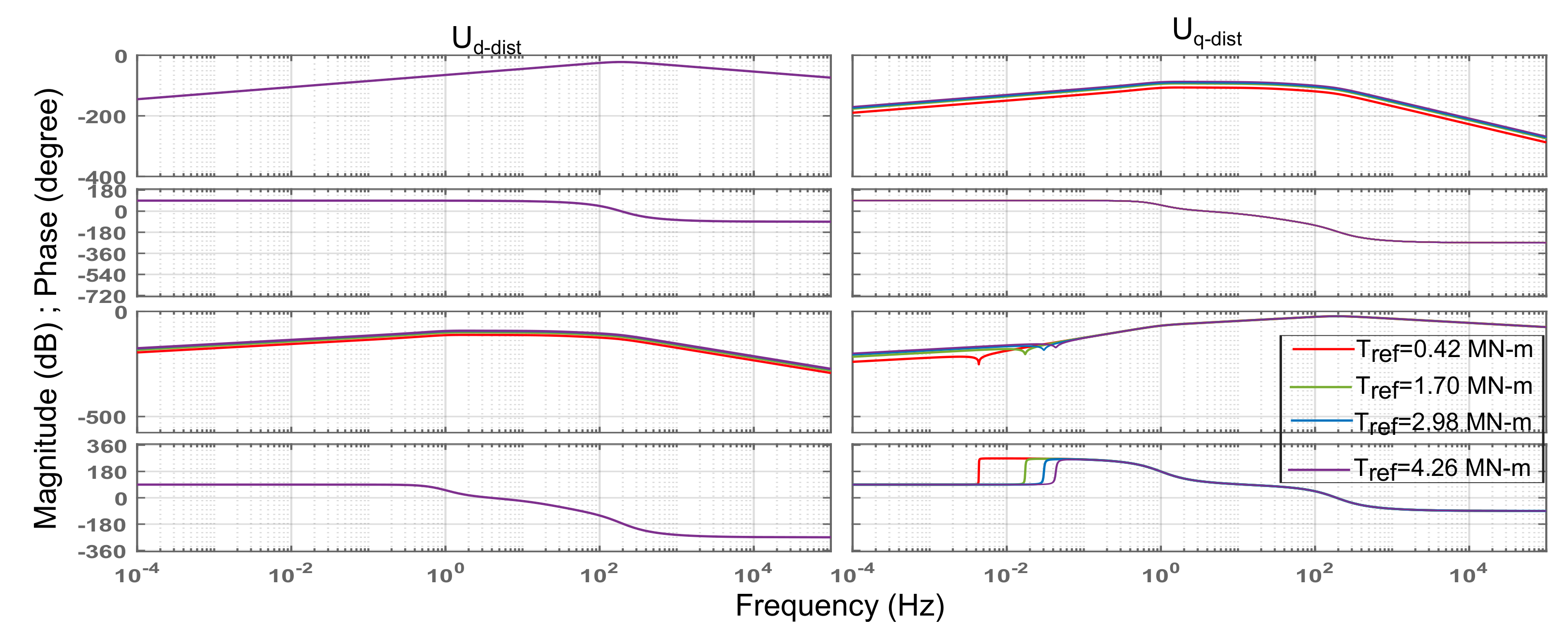
6. Frequency Domain Stability Analysis
6.1. Stability Analysis of Single Wind Turbine
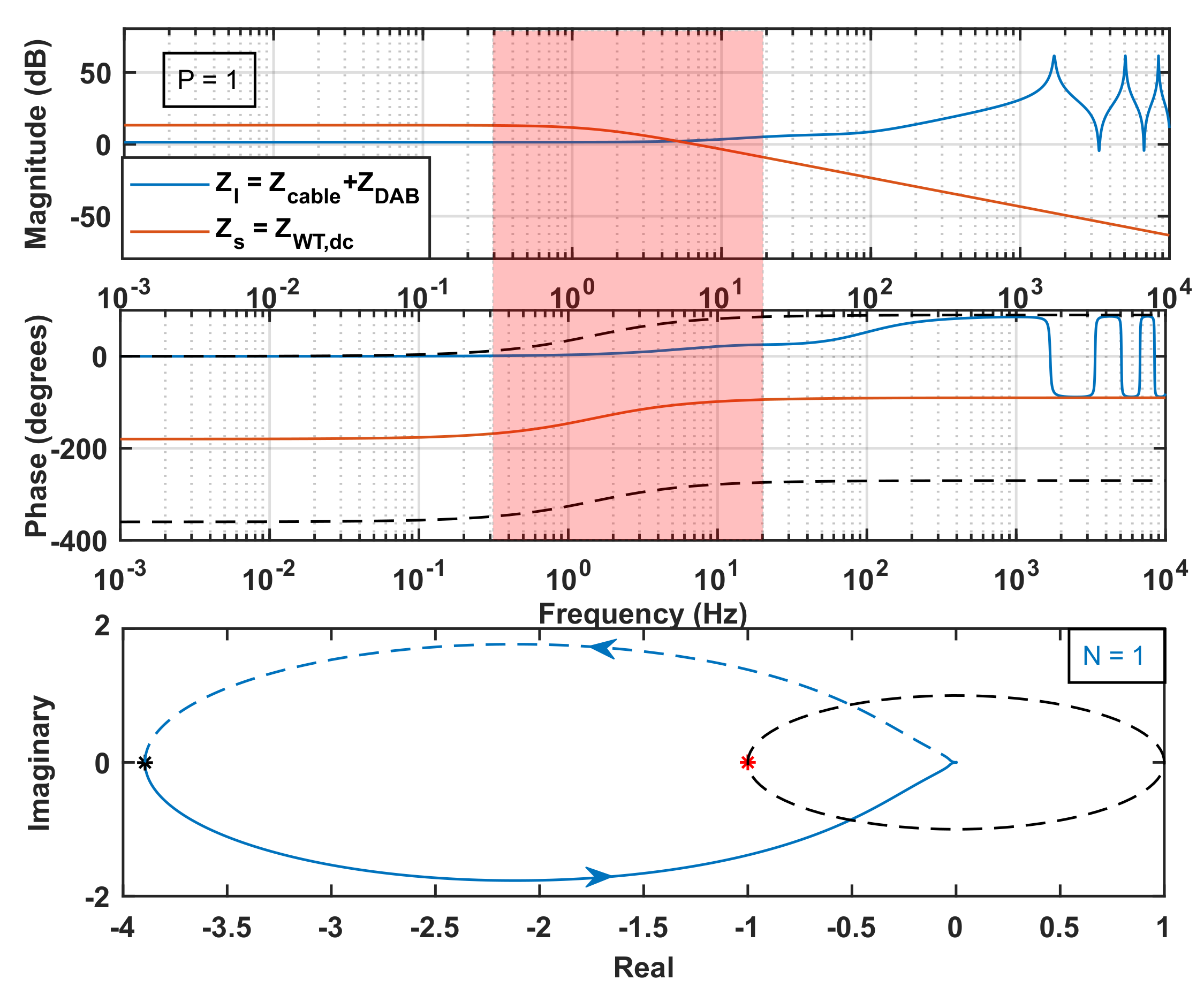
6.2. Star Configuration
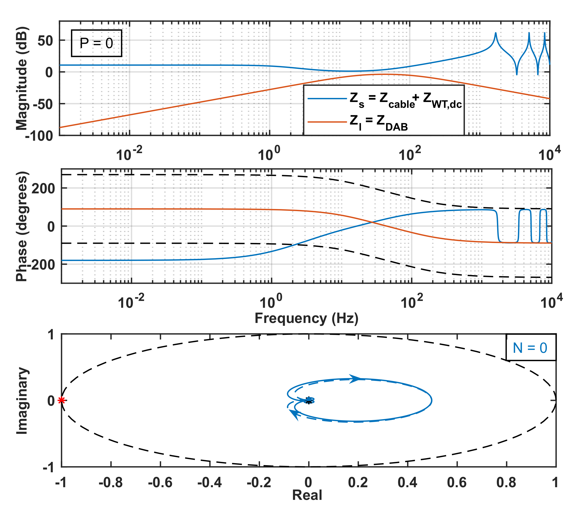
6.3. String Configuration
7. Conclusions
Author Contributions
Funding
Institutional Review Board Statement
Informed Consent Statement
Data Availability Statement
Conflicts of Interest
References
- Lundberg, S. Wind Farm Configuration and Energy Efficiency Studies-Series DC Versus AC Layouts; Chalmers University of Technology: Gothenburg, Sweden, 2006. [Google Scholar]
- Engel, S.P.; Stieneker, M.; Soltau, N.; Rabiee, S.; Stagge, H.; De Doncker, R.W. Comparison of the modular multilevel DC converter and the dual-active bridge converter for power conversion in HVDC and MVDC grids. IEEE Trans. Power Electron. 2014, 30, 124–137. [Google Scholar] [CrossRef]
- Lakshmanan, P.; Liang, J.; Jenkins, N. Assessment of collection systems for HVDC connected offshore wind farms. Electr. Power Syst. Res. 2015, 129, 75–82. [Google Scholar] [CrossRef] [Green Version]
- Wei, Q.; Wu, B.; Xu, D.; Zargari, N. Overview of offshore wind farm configurations. In IOP Conference Series: Earth and Environmental Science; IOP Publishing: Bristol, UK, 2017; Volume 93, p. 012009. [Google Scholar]
- Bahirat, H.J.; Mork, B.A.; Høidalen, H.K. Comparison of wind farm topologies for offshore applications. In Proceedings of the 2012 IEEE Power and Energy Society General Meeting, San Diego, CA, USA, 22–26 July 2012; IEEE: Piscataway, NJ, USA, 2012; pp. 1–8. [Google Scholar]
- Biskoping-ABB’Schweiz’AG. HVDC Circuit Breaker Switchyard. European EP3540750A1, 18 September 2019. [Google Scholar]
- Khersonsky, Y.; Ericsen, T.; Bishop, P.; Amy, J.; Andrus, M.; Baldwin, T.; Bartolucci, B.; Benavides, N.; Boroyevich, D.; Chaudhary, A.; et al. Recommended Practice for 1 to 35 kV Medium Voltage DC Power Systems on Ships; IEEE: Piscataway, NJ, USA, 2010. [Google Scholar]
- Abeynayake, G.; Li, G.; Liang, J.; Cutululis, N.A. A Review on MVdc Collection Systems for High-Power Offshore Wind Farms. In Proceedings of the 2019 14th Conference on Industrial and Information Systems (ICIIS), Kandy, Sri Lanka, 18–20 December 2019; IEEE: Piscataway, NJ, USA, 2019; pp. 407–412. [Google Scholar]
- Lyu, J.; Cai, X.; Molinas, M. Frequency domain stability analysis of MMC-based HVDC for wind farm integration. IEEE J. Emerg. Sel. Top. Power Electron. 2015, 4, 141–151. [Google Scholar] [CrossRef] [Green Version]
- Amin, M.; Rygg, A.; Molinas, M. Self-synchronization of wind farm in an MMC-based HVDC system: A stability investigation. IEEE Trans. Energy Convers. 2017, 32, 458–470. [Google Scholar] [CrossRef]
- Freijedo, F.D.; Rodriguez-Diaz, E.; Dujic, D. Stable and passive high-power dual active bridge converters interfacing MVDC grids. IEEE Trans. Ind. Electron. 2018, 65, 9561–9570. [Google Scholar] [CrossRef] [Green Version]
- Liu, B.; Li, Z.; Zhang, X.; Dong, X.; Liu, X. Impedance-Based Analysis of Control Interactions in Weak-Grid-Tied PMSG Wind Turbines. IEEE J. Emerg. Sel. Top. Circuits Syst. 2020, 11, 90–98. [Google Scholar] [CrossRef]
- Zhou, W.; Wang, Y.; Chen, Z. Reduced-order modelling method of grid-connected inverter with long transmission cable. In Proceedings of the IECON 2018-44th Annual Conference of the IEEE Industrial Electronics Society, Washington, DC, USA, 21–23 October 2018; IEEE: Piscataway, NJ, USA, 2018; pp. 4383–4389. [Google Scholar]
- Sun, J. Impedance-based stability criterion for grid-connected inverters. IEEE Trans. Power Electron. 2011, 26, 3075–3078. [Google Scholar] [CrossRef]
- Riccobono, A.; Santi, E. Comprehensive review of stability criteria for DC power distribution systems. IEEE Trans. Ind. Appl. 2014, 50, 3525–3535. [Google Scholar] [CrossRef]
- Gurumurthy, S.K.; Uhl, R.; Pitz, M.; Ponci, F.; Monti, A. Non-Invasive Wideband-frequency Grid Impedance Measurement Device. In Proceedings of the 2019 IEEE 10th International Workshop on Applied Measurements for Power Systems (AMPS), Aachen, Germany, 25–27 September 2019; IEEE: Piscataway, NJ, USA, 2019; pp. 1–6. [Google Scholar]
- Monti, A.; Gurumurthy, S.K.; Uhl, R.; Pitz, M. Vorrichtung zur Bestimmung der Impedanz in Abhängigkeit der Frequenz eines zu messenden Versorgungsnetzes. Patent DE 102019214533, 25 March 2021. [Google Scholar]
- Liao, Y.; Wang, X. Impedance-based stability analysis for interconnected converter systems with open-loop RHP poles. IEEE Trans. Power Electron. 2019, 35, 4388–4397. [Google Scholar] [CrossRef] [Green Version]
- Liu, X.; Islam, S. Reliability issues of offshore wind farm topology. In Proceedings of the 10th International Conference on Probablistic Methods Applied to Power Systems, Rincon, PR, USA, 25–29 May 2008; IEEE: Piscataway, NJ, USA, 2008; pp. 1–5. [Google Scholar]
- Zarkov, Z.; Demirkov, B. Power control of PMSG for wind turbine using maximum torque per ampere strategy. In Proceedings of the 2017 15th International Conference on Electrical Machines, Drives and Power Systems (ELMA), Sofia, Bulgaria, 1–3 June 2017; IEEE: Piscataway, NJ, USA, 2017; pp. 292–297. [Google Scholar]
- Doncker, R.W.D. Advanced Electrical Drives: Analysis, Modeling, Control; Springer: Berlin, Germany, 2011. [Google Scholar]
- Cupelli, M.; Gurumurthy, S.K.; Bhanderi, S.K.; Yang, Z.; Joebges, P.; Monti, A.; De Doncker, R.W. Port controlled Hamiltonian modeling and IDA-PBC control of dual active bridge converters for DC microgrids. IEEE Trans. Ind. Electron. 2019, 66, 9065–9075. [Google Scholar] [CrossRef]


Publisher’s Note: MDPI stays neutral with regard to jurisdictional claims in published maps and institutional affiliations. |
© 2021 by the authors. Licensee MDPI, Basel, Switzerland. This article is an open access article distributed under the terms and conditions of the Creative Commons Attribution (CC BY) license (https://creativecommons.org/licenses/by/4.0/).
Share and Cite
Biskoping, M.; Kadam, T.; Gurumurthy, S.K.; Ponci, F.; Monti, A. Comparison of Star and String Offshore DC Collector Grid Topologies on the Aspect of Stability—An Impedance Approach. Energies 2021, 14, 6253. https://doi.org/10.3390/en14196253
Biskoping M, Kadam T, Gurumurthy SK, Ponci F, Monti A. Comparison of Star and String Offshore DC Collector Grid Topologies on the Aspect of Stability—An Impedance Approach. Energies. 2021; 14(19):6253. https://doi.org/10.3390/en14196253
Chicago/Turabian StyleBiskoping, Matthias, Tanmay Kadam, Sriram Karthik Gurumurthy, Ferdinanda Ponci, and Antonello Monti. 2021. "Comparison of Star and String Offshore DC Collector Grid Topologies on the Aspect of Stability—An Impedance Approach" Energies 14, no. 19: 6253. https://doi.org/10.3390/en14196253
APA StyleBiskoping, M., Kadam, T., Gurumurthy, S. K., Ponci, F., & Monti, A. (2021). Comparison of Star and String Offshore DC Collector Grid Topologies on the Aspect of Stability—An Impedance Approach. Energies, 14(19), 6253. https://doi.org/10.3390/en14196253