
A Topology Optimization Based Design of Space Radiator for Focal Plane Assemblies


Abstract
:1. Introduction
2. Thermal Analysis of the Radiator Design Problem
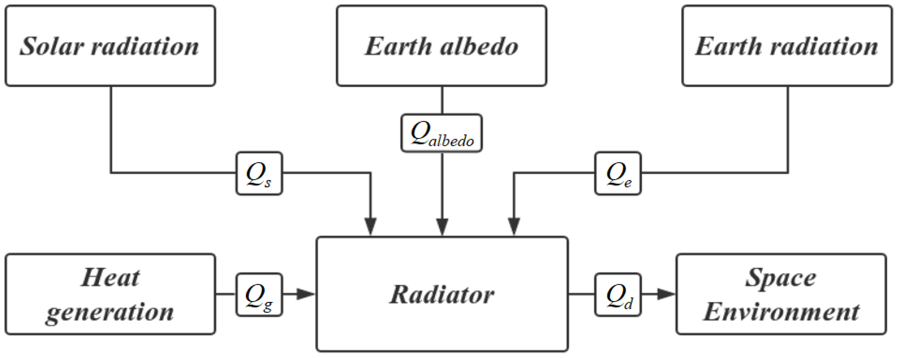
2.1. Thermal Environment of the Radiator
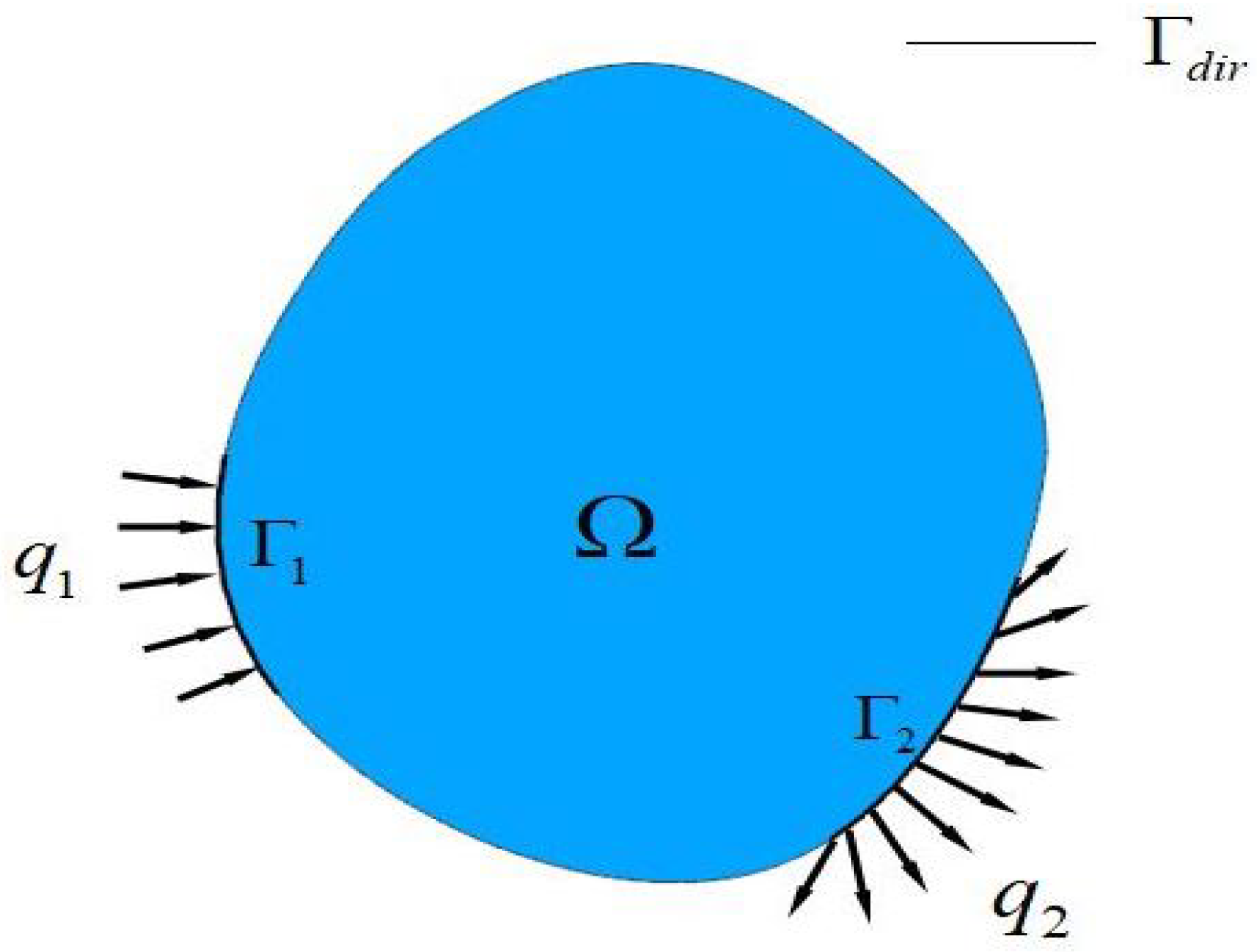
2.2. Generalization of the Governing Equations and Boundaries of Radiator Design Problems
3. Formation of the Topology Optimization Model
3.1. SIMP Model
3.2. Formation of the Optimization Objective
3.3. Finite Element Solution of the Problem
3.4. Formation of Mathematical Model
3.5. Optimization Design Work Flow
4. Optimization Design of the Radiator
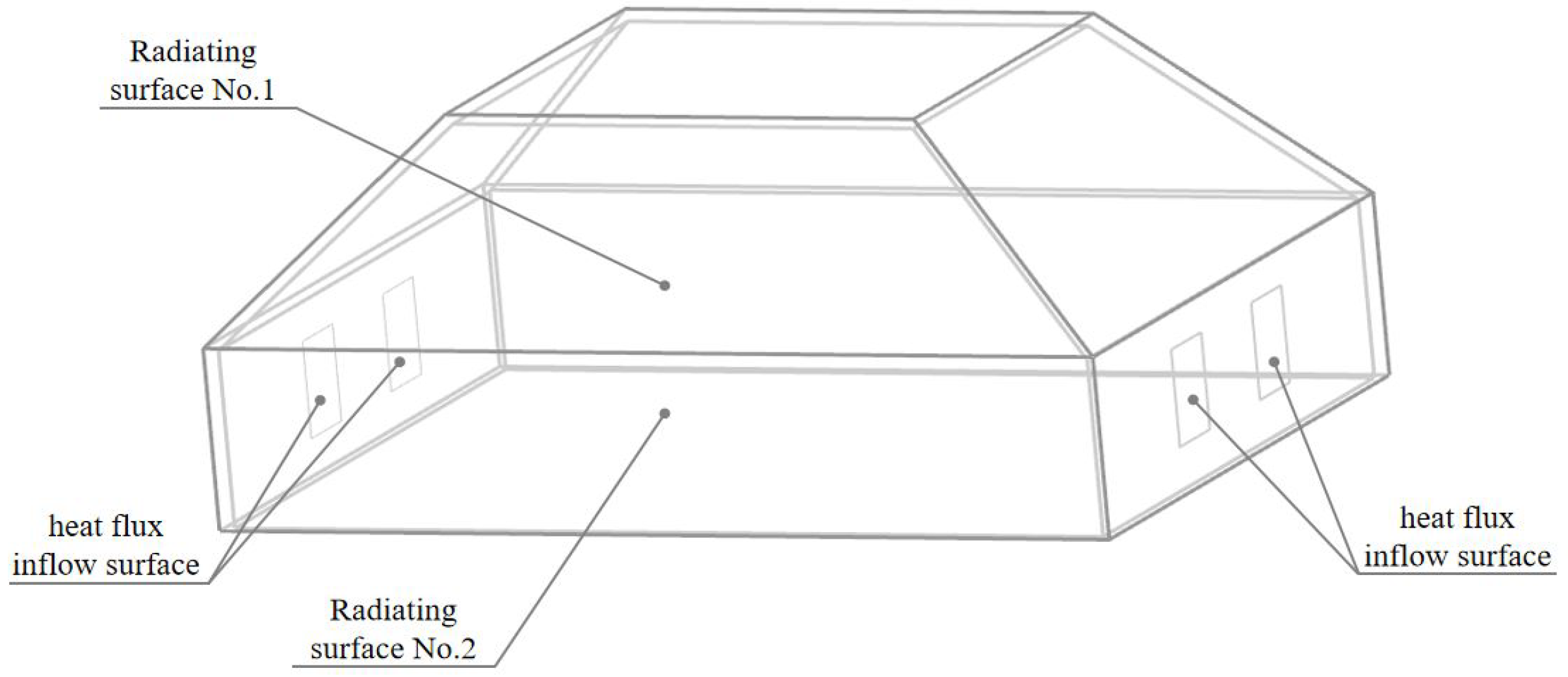
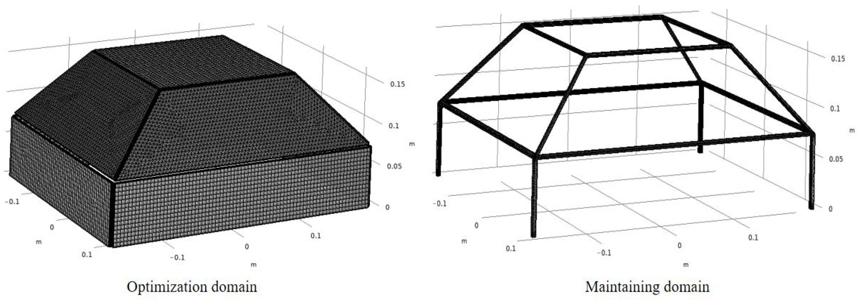
4.1. Initial Design of the Radiator
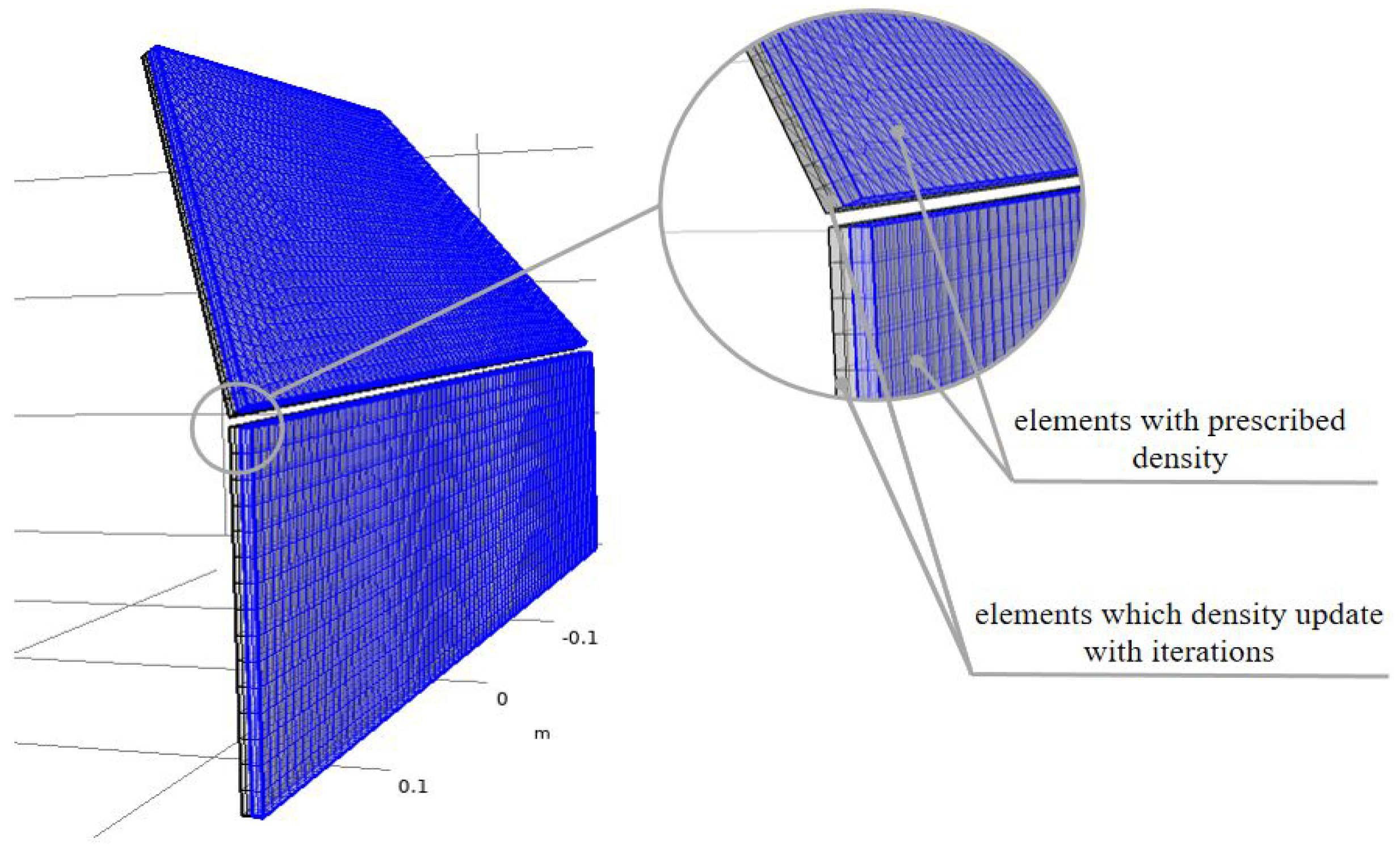
4.2. Mesh Configuration
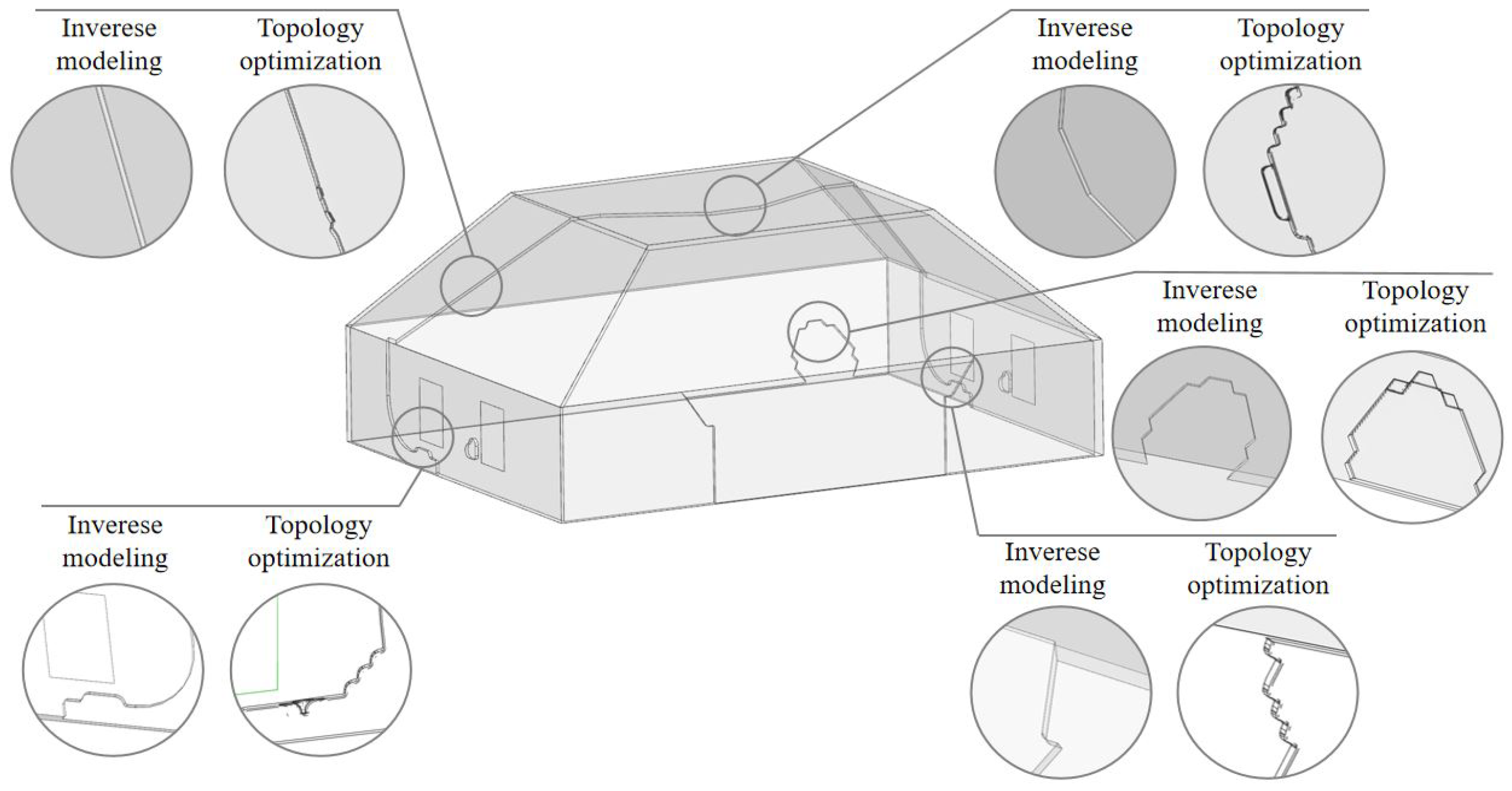
4.3. Topology Optimization Result of Maximal Thermal Stiffness Design
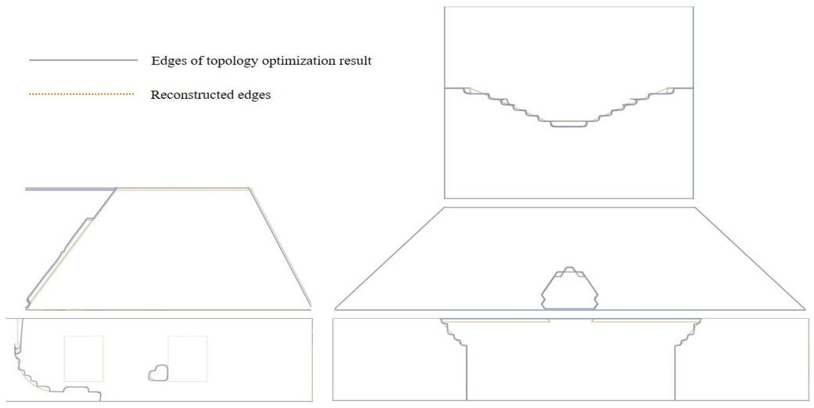
4.4. Reconstruction of the Radiator
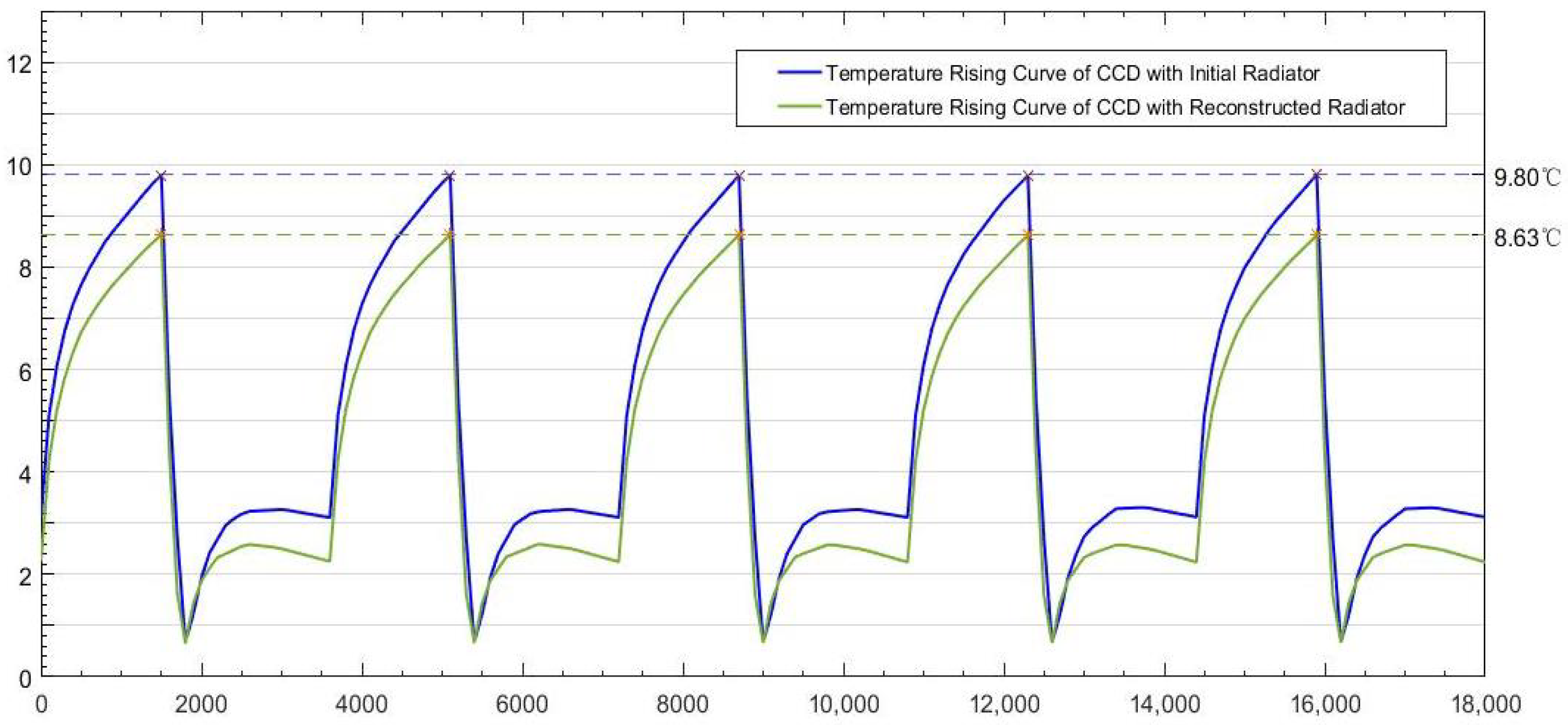
4.5. Transient Thermal State Simulation
4.6. Results
5. Conclusions
- (1)
- The objective of maximal thermal stiffness formed in this paper could describe influences of coupled conduction and radiation on the radiator.
- (2)
- Inverse modeling based on the result of topology optimization could improve manufacturability. As the maximal temperature on reconstructed radiator increases by 0.033 °C compared to topology optimization result, the heat dissipation efficiency improvement by topology optimization could be retained to a great extent after reconstruction.
- (3)
- The transient simulation results indicate that heat dissipation efficiency is improved on reconstructed radiator, as an average decrease of 1.167 °C of maximal temperature on CCD assemblies in working durations is achieved compared to those with initial radiator. The improvement makes a longer working duration per cycle possible under the same temperature limits.
Author Contributions
Funding
Institutional Review Board Statement
Informed Consent Statement
Data Availability Statement
Conflicts of Interest
Nomenclature
| solar radiation absorption | |
| earth radiation absorption | |
| albedo absorption | |
| external heat flow generated by power-consuming sensors | |
| the energy that radiating into space environment | |
| time dependent energy change within the radiator | |
| solar radiation absorptance | |
| view factor of solar radiation | |
| solar constant | |
| earth radiation absorptance | |
| view factor of earth radiation | |
| earth radiation | |
| view factor of albedo | |
| A | area of the radiator |
| ,, | isotropical thermal conductivity |
| earth albedo | |
| view factor of the radiating surface to the space | |
| hemispherical emittance | |
| Stefan–Boltzmann constant | |
| outer surface of the domain | |
| ambient temperature | |
| Lagrange multiplier | |
| optimization domain | |
| T | temperature field on radiator |
| C | specific heat capacity |
| density | |
| m | mass of the radiator |
| t | time |
| n | number of element nodes |
| element nodal temperature vector | |
| global heat conduction matrix | |
| global thermal radiation matrix | |
| nodal temperature vector | |
| global thermal load vector | |
| artificial density | |
| u | virtual temperature |
| objective function of max thermal stiffness | |
| equivalent objective function | |
| thermal load | |
| prescribed working temperature | |
| total thermal resistance | |
| p | penalty |
References
- Xu, X.; Li, Z.; Xue, L. Analysis and processing of CCD noise. Infrared Laser Eng. 2004, 33, 343–357. [Google Scholar]
- Ahmad, A.; Arndt, T.; Gross, R.; Hahn, M.; Panasiti, M. Structural and thermal modeling of a cooled CCD camera. Proc. SPIE Int. Soc. Opt. Eng. 2001, 4444, 122–129. [Google Scholar]
- Jian, C. Research of CMOS Image Sensor. Electron. Sci. Technol. 2007, 144, 73–76. [Google Scholar]
- Chen, L.H.; Li, Y.C.; Luo, Z.T.; Dong, J.H.; Wang, Z.S.; Xu, S.Y. Thermal design and testing of CCD for space camera. Opt. Precis. Eng. 2011, 19, 2117–2122. [Google Scholar] [CrossRef]
- Sarafraz, M.M.; Dareh Baghi, A.; Safaei, M.R.; Leon, A.S.; Ghomashchi, R.; Goodarzi, M.; Lin, C.-X. Assessment of Iron Oxide (III)–Therminol 66 Nanofluid as a Novel Working Fluid in a Convective Radiator Heating System for Buildings. Energies 2019, 12, 4327. [Google Scholar] [CrossRef] [Green Version]
- Bagherzadeh, S.A.; Jalali, E.; Sarafraz, M.M.; Akbari, O.A.; Karimipour, A.; Goodarzi, M.; Bach, Q.-V. Effects of magnetic field on micro cross jet injection of dispersed nanoparticles in a microchannel. Int. J. Numer. Methods Heat Fluid Flow 2019, 30, 2683–2704. [Google Scholar] [CrossRef]
- Han, D.; Wu, Q.W.; Lu, E.; Chen, L.H.; Yang, C.Y. Thermal design of CCD focal plane assemblies for attitude-varied space cameras. Opt. Precis. Eng. 2009, 17, 2665–2671. [Google Scholar]
- Chen, E.T.; Lu, E.; Chen, L.H.; Yang, C.Y. Thermal engineering design of CCD component of space remote-sensor. Opt. Precis. Eng. 2000, 8, 523–526. [Google Scholar]
- Wu, Q.W.; Guo, L. Thermal design and proof tests of CCD components in spectral imagers. Opt. Precis. Eng. 2009, 17, 2441–2444. [Google Scholar]
- Zi, K.M.; Wu, Q.W.; Guo, J.; Luo, Z.T.; Chen, L.H.; Li, M. Thermal design of CCD focal plane assembly of space optical remote-sensor. Opt. Tech. 2008, 34, 401–407. [Google Scholar]
- Fan, G.; Duan, B.; Zhang, Y.; Ji, X.; Qian, S. Thermal control strategy of OMEGA SSPS based simultaneous shape and topology optimization of butterfly wing radiator. Int. Commun. Heat Mass Transf. 2020, 119, 104912. [Google Scholar] [CrossRef]
- da Silva, D.F.; Muraoka, I.; de Sousa, F.L.; Garcia, E.C. Multiobjective and Multicase Optimization of a Spacecraft Radiator. J. Aerosp. Technol. Manag. 2019, 11, e0518. [Google Scholar] [CrossRef]
- Kim, T.Y.; Chang, S.Y.; Yong, S.S. Optimizing the Design of Space Radiators for Thermal Performance and Mass Reduction. J. Aerosp. Eng. 2016, 30, 04016090. [Google Scholar] [CrossRef]
- Jiang, F.; Wu, Q.; Wang, Z.; Liu, J.; Deng, H. Thermal design and analysis of high power star sensors. Case Stud. Therm. Eng. 2015, 6, 52–60. [Google Scholar] [CrossRef] [Green Version]
- Bendsøe, M.P.; Noboru, K. Generating optimal topologies in structural design using a homogenization method. Comput. Methods Appl. Mech. Eng. 1998, 71, 197–224. [Google Scholar] [CrossRef]
- Haslinger, J.; Hillebrand, A.; Kärkkäinen, T.; Miettinen, M. Optimization of conducting structures by using the homogenization method. Struct. Multidiscip. Optim. 2002, 24, 125–140. [Google Scholar] [CrossRef]
- Bendsøe, M.P. Optimal shape design as a material distribution problem. Struct. Optim. 1989, 1, 193–202. [Google Scholar] [CrossRef]
- Cho, S.; Choi, J.Y. Efficient topology optimization of thermo-elasticity problems using coupled field adjoint sensitivity analysis method. Finite Elem. Anal. Des. 2005, 41, 1481–1495. [Google Scholar] [CrossRef]
- Bendsøe, M.; Sigmund, O. Topology Optimization—Theory, Methods and Applications; Springer: Berlin/Heidelberg, Germany, 2003; pp. 2–62. [Google Scholar]
- Iga, A.; Nishiwaki, S.; Izui, K.; Yoshimura, M. Topology optimization for thermal conductors considering design-dependent effects, including heat conduction and convection. Int. J. Heat Mass Transf. 2009, 52, 2721–2732. [Google Scholar] [CrossRef]
- Joe, A.; Ole, S.; Niels, A. Large scale three-dimensional topology optimisation of heat sinks cooled by natural convection. Int. J. Heat Mass Transf. 2016, 100, 876–891. [Google Scholar]
- Yin, L.; Ananthasuresh, G.K. A novel topology design scheme for the multi-physics problems of electro-thermally actuated compliant micromechanisms. Sens. Actuators A Phys. 2009, 97, 599–609. [Google Scholar]
- Xie, Y.M.; Steven, G.P. Evolutionary Structural Optimization; Springer: Lodon, UK, 1997; pp. 12–61. [Google Scholar]
- Qing, L.I.; Steven Grant, P.; Querin Osvaldo, M. Shape and topology design for heat conduction by Evolutionary Structural Optimization. Int. J. Heat Mass Transf. 1999, 42, 3361–3371. [Google Scholar]
- Castro, D.A.; Kiyono, C.Y.; Silva, E.C.N. Design of radiative enclosures by using topology optimization. Int. J. Heat Mass Transf. 2015, 88, 880–890. [Google Scholar] [CrossRef]
- Ming, G.R.; Guo, S. Thermal Control of Spacecraft, 2nd ed.; Science Press: Beijing, China, 1998; pp. 5–56. [Google Scholar]
- Gunga, H.C.; Steinach, M.; Werner, A.; Kirsch, K.A. Handbook of Space Technology; Wiley: West Sussex, UK, 2009; pp. 33–51. [Google Scholar]
- Yang, S.M.; Tao, W.Q. Heat Transfer, 4th ed.; Beijing Higher Education Press: Beijing, China, 1998; pp. 20–118. [Google Scholar]
- Niu, F.; Xu, S.L.; Cheng, G.D. A general formulation of structural topology optimization for maximizing structural stiffness. Struct. Multidipl. Optim. 2011, 43, 561–572. [Google Scholar] [CrossRef]
- Bruns, T.E. Topology optimization of convection-dominated, steady-state heat transfer problems. Int. J. Heat Mass Transf. 2007, 50, 2859–2873. [Google Scholar] [CrossRef]
- Qi, Y.; He, Y.; Zhang, W.; Guo, J. Thermal analysis and design of electronic equipments. Mod. Electron. Technol. 2003, 144, 73–76. [Google Scholar]
- Svanberg, K. The method of moving asymptotes—A new method for structural optimization. Int. J. Numer. Methods Eng. 2010, 24, 359–373. [Google Scholar] [CrossRef]
- Sophie, D. Radiation effects on electronic devices in space. Aerospaceence Technol. 2005, 9, 93–99. [Google Scholar]


| Material | Conductivity (W/(m · K)) | Density (kg/m3) | Specific Heat Capacity (J/(kg · K)) |
|---|---|---|---|
| Aluminum | 155 | 2700 | 900 |
| Heat conductive gasket | 3.5 | / | / |
| Silver foil | 400 | 10,530 | 230 |
| Heat conductive grease | 1.5 | / | / |
| Load (W) | Maximal Temperature (°C) | Minimal Temperature (°C) | Weight (kg) |
|---|---|---|---|
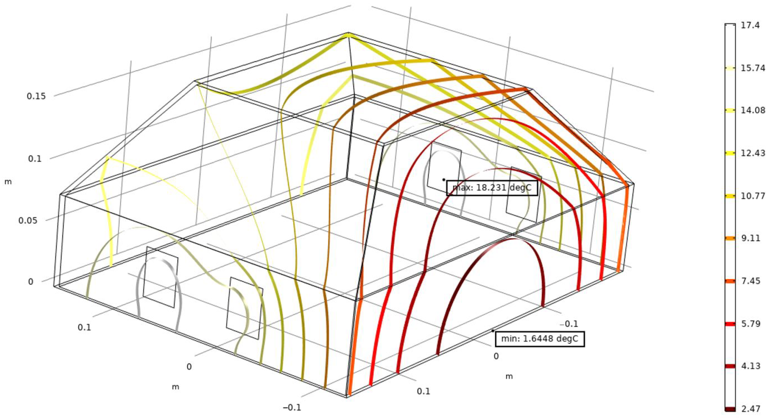
| 16 | 18.231 | 1.645 | 2.026 |
| Load (W) | Maximal Temperature (°C) | Minimal Temperature (°C) | Weight (kg) |
|---|---|---|---|
| 16 | 15.601 | 1.480 | 2.048 |
| Design | Max Temperature (°C) | Min Temperature (°C) | Weight (kg) |
|---|---|---|---|
| Initial design | 18.231 | 1.645 | 2.011 |
| Topology optimization | 15.601 | 1.480 | 2.048 |
| Reconstructed radiator | 15.634 | 1.489 | 2.029 |
| Time (s) | 1500 | 5100 | 8700 | 12,300 | 15,900 |
|---|---|---|---|---|---|
| Max temperature on CCD with initial radiator (°C) | 9.793 | 9.792 | 9.787 | 9.787 | 9.805 |
| Max temperature on CCD with reconstructed radiator (°C) | 8.634 | 8.627 | 8.629 | 8.620 | 8.619 |
Publisher’s Note: MDPI stays neutral with regard to jurisdictional claims in published maps and institutional affiliations. |
© 2021 by the authors. Licensee MDPI, Basel, Switzerland. This article is an open access article distributed under the terms and conditions of the Creative Commons Attribution (CC BY) license (https://creativecommons.org/licenses/by/4.0/).
Share and Cite
Shen, X.; Han, H.; Li, Y.; Yan, C.; Mu, D. A Topology Optimization Based Design of Space Radiator for Focal Plane Assemblies. Energies 2021, 14, 6252. https://doi.org/10.3390/en14196252
Shen X, Han H, Li Y, Yan C, Mu D. A Topology Optimization Based Design of Space Radiator for Focal Plane Assemblies. Energies. 2021; 14(19):6252. https://doi.org/10.3390/en14196252
Chicago/Turabian StyleShen, Xiao, Haitao Han, Yancheng Li, Changxiang Yan, and Deqiang Mu. 2021. "A Topology Optimization Based Design of Space Radiator for Focal Plane Assemblies" Energies 14, no. 19: 6252. https://doi.org/10.3390/en14196252
APA StyleShen, X., Han, H., Li, Y., Yan, C., & Mu, D. (2021). A Topology Optimization Based Design of Space Radiator for Focal Plane Assemblies. Energies, 14(19), 6252. https://doi.org/10.3390/en14196252