Abstract
Transparent, objective, and repeatable resource assessments should be the goal of companies, investors, and regulators. Different types of resources, however, may require different approaches for their quantification. In particular, coal can be treated both as a solid resource (and thus be mined) as well as a reservoir for gas (which is extracted). In coal mining, investment decisions are made based on a high level of data and establishment of seam continuity and character. The Australasian Code for Reporting of Exploration Results, Mineral Resources and Ore Reserves (the JORC Code) allows deposits to be characterised based on the level of geological and commercial certainty. Similarly, the guidelines of the Petroleum Resource Management System (PRMS) can be applied to coal seam gas (CSG) deposits to define the uncertainty and chance of commercialisation. Although coal and CSG represent two very different states of resources (i.e., solid vs. gaseous), their categorisation in the JORC Code and PRMS is remarkably similar at a high level. Both classifications have two major divisions: resource vs. reserve. Generally, in either system, resources are considered to have potential for eventual commercial production, but this has not yet been confirmed. Reserves in either system are considered commercial, but uncertainty is still denoted through different subdivisions. Other classification systems that can be applied to CSG also exist, for example the Canadian Oil and Gas Evaluation Handbook (COGEH) and the Chinese Standard (DZ/T 0216-2020) and both have similar high-level divisions to the JORC Code and PRMS. A hypothetical case study of a single area using the JORC Code to classify the coal and PRMS for the gas showed that the two methodologies will have overlapping, though not necessarily aligned, resource and reserve categories.
1. Introduction
When hydrocarbon resources are referred to as either conventional or unconventional what is really being referenced is the maturity of knowledge on how to develop those reservoirs. For the last 150 years the oil and, later, natural gas industries have exploited high permeability reservoirs that have accumulated hydrocarbons in structural and stratigraphic traps. Now, the search for hydrocarbons includes very low permeability strata where new technologies must be employed to extract them at economic rates. As the world transitions to a higher proportion of renewable energy, it will remain important to characterise and quantify resources such as gas and coal, as countries will wish to maintain ongoing energy security during the transition, especially in times of uncertainty, such as the pandemic of 2020–2021 and beyond.
Coal is unique among gas reservoirs because it can also be mined as a solid material. The techniques and standards for the estimation of mineral resources and reserves, including coal, are different from those for estimation of oil and gas volumes. Minerals resource estimation standards have fairly stringent criteria, mandating that, before the point of a final investment decision to develop a mine, volumes and quality be determined to a high level of confidence. To be economically viable, a mining project must typically operate throughout one or more price cycles, which often includes a sustained period of low prices. Companies, government regulators, and especially investors need assurance that there are enough resources at specific quality levels and defined capital and operating costs to be commercial throughout the mine’s life. Thus, mining companies and their investors are relatively risk-averse and historically have probably had lower tolerance for uncertainties than, say, petroleum companies, and this is reflected in the resource and reserve estimation standards for minerals, hereinafter referred to as codes. In contrast, historically, the oil and gas industry began with a higher appetite for risk. Profit margins of successful conventional oil and gas projects are typically larger than those of mining projects.
While the classification of coal resources and reserves follows the same standards as other minerals, the estimation techniques and resource classifications when applied to coal reflect the commodity’s geological controls. The differences in resource estimation and classification techniques between petroleum and coal therefore also reflect the fundamentally different geological controls of the two commodities. Coal occurs as distinct layers whose thickness, quality, and lateral continuity are controlled by stratigraphy and structure. Conventional petroleum deposits are also highly influenced by stratigraphy and structure, but because the hydrocarbons need to migrate and accumulate in a trap there is an extra level of complexity in their discovery and estimation of volumes compared to coal. There are of course huge differences also between the geology of coal and of metallic minerals such as gold, copper, and uranium, which are all covered by the same mineral estimation code; however, the codes are not prescriptive in defining actual estimation techniques. In addition, there are commodity-specific clauses within the codes, and, in the case of coal, associated guidelines to the Australasian Code for Reporting of Exploration Results, Mineral Resources and Ore Reserves [1], hereon referred to as the JORC Code.
Finally, how minerals and petroleum are extracted also determines how their resources and reserves are assessed. For example, for coal, the quality and thickness are “static” in the sense that, although these properties are quite heterogeneous having both vertical and lateral variability, they do not change over time and certainly not within the time frame of mining. Coal is also a “static” resource in the sense that every tonne mined has a specific geospatial location and that does not change, that is, unlike petroleum, the resource does not migrate to a different location (i.e., a drillhole) where it is extracted.
In contrast to coal, a petroleum deposit is relatively homogeneous. Although different gas deposits may have different qualities, the quality within a single gas field tends to remain roughly the same throughout most of its extraction, at least until the field nears depletion. Unlike coal, the gas is “dynamic” and will mix within the reservoir, resulting in a relatively uniform composition.
When gassy, a coal seam is considered an unconventional reservoir for a few reasons: 1. the permeability of coal is low (compared to sandstones, for example), 2. coal is a source as well as a reservoir (and thus is considered to be a “continuous reservoir”), 3. a coal reservoir needs to be de-pressured through de-watering before gas will flow, and 4. gas generated from coal (referred to here as “coal seam gas”, CSG) can be biogenic or thermogenic in origin. The most widely used system to estimate gas in coal is the Petroleum Resource Management System (PRMS) [2,3,4]; however the Canadian Oil and Gas Evaluation Handbook (COGEH) [5] is also commonly employed, as is the Chinese Standard [6], for deposits within China or Chinese companies reporting their assets to their government. Thus, it is these three classification schemes that will be summarized and compared in this paper, although the latter two will only have a precursory review compared to the PRMS. The goal will be to make broad comparisons, and we recognise that our interpretations and assertions may differ from others. There are, of course, other coal and coal seam gas resource classification systems, such as those used by the U.S. Geological Survey [7,8,9]. Although brilliant at addressing geological risk, they do not explicitly address commercial risk nor are they accepted by most major stock market exchanges.
In the case of coal, relatively standardised codes for the public estimating of resources and reserves have been developed over recent decades and are now applied in most countries with a significant mining industry. This development began with the JORC Code for public reporting of mineral resources and reserves in Australia and New Zealand, first released in 1989. With the globalisation of the mining industry, and improved regulation and reporting standards, an international committee (the Committee for Mineral Reserves International Reporting Standards, or CRIRSCO) was formed in 1994, and by 2006 it had released a template to be used by professional organisations developing national standards for their own countries, known as the CRIRSCO template (which was later modified). The key aspects of the JORC Code and the CRIRSCO template are almost identical, as are those of the many national codes that were later developed. As the CRIRSCO document is a template, not a binding code, this paper will focus on the closely related JORC Code, which was developed for reporting of all minerals but also refers to non-binding guidelines specific to the estimation of coal resources.
Ultimately, the audience for this paper are CSG and coal mining professionals who want to understand how the different classifications estimate the same commodity, whether it is the tonnage of coal or the volume of gas in coal. This paper may be of little help to professionals who use one or the other classification system routinely, but it is hoped that it will give insight to those less familiar with coal and/or CSG assessments. Thus, the purpose of this paper relative to coal and CSG deposits is to:
- Summarise the JORC system of coal resource and reserve classification,
- Summarise the PRMS, COGEH, and Chinese Standard of resource and reserve classification,
- Compare points of differences and similarity of how these two sets (i.e., JORC Code vs. PRMS, COGEH, and Chinese Standard) of standards classify uncertainty and commerciality of a deposit, and
- Conduct a simple test case that uses the same data to calculate resources using both the JORC Code (coal) and the PRMS (gas).
There are two important caveats for this paper that readers should bear in mind. Firstly, the relevant codes, guidelines, and supporting documents prepared by the relevant professional organisations should always be consulted for detail and context before any assessments are conducted. This paper gives a perspective, formed from the usage of these codes by the authors, and is not meant to be definitive but rather demonstrative. Secondly, both authors come from an exploration background and thus it is through that prism which both coal and gas resources are generally viewed and thus more heavily presented in this paper.
2. Classification of Coal Resources and Reserves from the Perspective of Mining
2.1. The International Codes
As mentioned, the first of the modern codes for estimation of mineral resources and reserves was the JORC Code of Australia and New Zealand, which was initially released in 1989. The CRIRSCO template was developed later, and “CRIRSCO-like” standardised national codes developed in other countries/regions, including the USA, Russia, Europe, Brazil, Canada, Indonesia, South Africa, the Philippines, Chile, and Colombia, covering most of the countries with a significant mining industry. These codes, and the JORC Code, can all be referred to as “CRIRSCO-like” codes. They share common definitions of terms like “resource” and “reserve” and share the three principles that guide the use of the code. The codes have been updated with improvements every few years. Standardisation of the codes is important with globalisation, making it easier for investors to evaluate and compare projects and for technical people to work across borders. To avoid duplication, the focus of subsequent discussions will be on the JORC Code as an example.
2.2. The JORC Code
The JORC Code is mandated for public reporting of exploration results, mineral resources, and mineral reserves in Australia and New Zealand. The application of the Code has been described in detail by Miskelly and West [10]. The three principals that guide the use of the code are:
- Transparency of information and data,
- Materiality—all information relevant to investors and their advisors must be included, and
- Competency—a qualified person, the Competent Person, must take responsibility for reporting under the code and must not remain silent on any aspect that is material to investors or their advisors [1]; the Competent Person is a member of and subject to the Code of Ethics of a suitable professional organisation and can be questioned and sanctioned by peers within this professional organisation if necessary; the Competent Person must have a minimum of 5 years relevant experience.
The JORC Code is not prescriptive. It is not a rulebook on the actual techniques to be used in estimating mineral resources and reserves. As noted by Coombes [11], “JORC has fiercely safeguarded any attempts to introduce prescriptive techniques and processes,” therefore, as noted by Stephenson and Miskelly [12] (as reported by Coombes [11]), “allowing Competent Persons considerable freedom to exercise their professional judgement, but ensuring they can be held to account for their actions.” The Competent Person, following industry best practices, decides the estimation techniques. The JORC Code focusses on clear definitions of the meaning of the terms “resource” and “reserve” and of their sub-categories and on describing the technical studies required for public reporting of resource and reserve volumes and quality. There is also a detailed check list covering the level of detail normally expected in the accompanying report, including topics such as the status of mineral tenements, the sampling techniques, integrity of the database, verification of analytical results, resource and reserve modelling techniques, and discussion of the level of accuracy of the results. The use of this checklist is prescriptive (“if not, why not?”) and has become a benchmark for Competent Persons to follow.
However, guidelines to the JORC Code of 2012 have been issued, specifically for coal, titled “Australian Guidelines for the Estimation and Classification of Coal Resources” [13], which will be referred to here as the Coal Guidelines. The JORC Code refers to these for guidance but cautions that “Competent Persons should, as always, exercise their judgement in the application of these guidelines to ensure they are appropriate to the circumstances being reported. They may not be appropriate to all situations in Australia or overseas.” In this context, the Coal Guidelines are meant to provide guidance on resource estimation techniques.
2.3. Points of Observation
The starting point for definition of resources and reserves is the definition of the Point of Observation, as the type and density of points of observation are integral to the definitions. They are well-defined in the Coal Guidelines, being data points (drillholes, trenches, channels, etc.) of two types:
Quality Points of Observation: Data where a section of the coal has been collected and analysed (e.g., drillholes, trenches) as channel samples in surface or underground workings. Cores taken by a drillhole should have a suitable level of core recovery to be regarded as a valid Quality Point of Observation.
Quantity Points of Observation: These are data that provide information on the seam by observation. Examples include boreholes with downhole geophysical logs that were not cores but where drill cuttings can be observed.
There are typically more quantity Points of Observation than those for quality. Quality Points, of course, are also valid as quantity points. Deposits with complicated structures will need infill Quantity Points. In the evaluation of deep underground coal, where the presence of faults or intrusives can be highly disruptive to longwall mining, closely spaced drilling to define their presence and extent may be impractical. A combination of drilling with seismic may be technically (and financially) the most effective. Seismic, gravity, and other geophysical surveys, and data from geological mapping, are regarded in the Coal Guidelines as “supportive data”.
2.4. Classification of Coal Resources
2.4.1. Coking and Thermal Coal
When discussing coal resources, it is important to note that there are two distinct uses. Thermal coal is used in power plants or other facilities to provide heat, for electricity generation (the majority of thermal coal), or for industrial processes (e.g., cement making). Coking coal is used as an ingredient for the blast furnace process of steel making and is higher priced than thermal coal. Thermal coal in small volumes may also be a lower quality by-product of mining and processing coking coal.
2.4.2. Coal Beneficiation
Coking coal generally goes through a process of beneficiation, using density separation to reduce the amount of higher density material, i.e., non-coal partings, seam roof, and seam floor. Thermal coal may be marketed as raw coal (unprocessed) into some markets, but higher-quality thermal coal is frequently also processed.
2.4.3. The Time Frame
The JORC Code definition of mineral resources includes the criteria of “reasonable prospects for eventual economic extraction” [1]. The JORC Code also clarifies that for coal and some other commodities the time frame of “eventual” may be up to 50 years. As a reality check, Davis and Radonich [14] have reviewed the huge changes in the Queensland mining industry over the last 50 years and have compared long-term coal price forecasts by well-established industry and government groups with the real-world volatility of coal prices over the medium term. In the case of thermal coals, such a prolonged timeframe may run up against the limits of an increasingly carbon-constrained global economy. For example, many industry analysts and stakeholders (e.g., [15]) predict a significant decline in global thermal coal utilisation over the next 30 years.
2.4.4. The Classifications
The quantity, quality, and continuity of a mineral resource is estimated or interpreted from geological evidence, including sampling. In practice, for a deposit to be considered as having reasonable prospects of eventual economic extraction, it is necessary to consider the mining technique and costs. Costs will vary greatly, for example, between a surface and underground mine. Other factors such as possible environmental issues, transport methods and costs, the likely market and coal price through a price cycle, and the infrastructure needed to transport the coal to market must all be considered.
The JORC Code also adds that “a Mineral Resource is not simply an inventory of all mineralisation drilled or sampled.” Furthermore, it states an assessment “is a realistic inventory of mineralisation which, under assumed and justifiable technical, economic, and development conditions, might in whole or in part become economically extractable.”
Mineral resources are further subdivided into the categories of inferred, indicated, and measured, depending on the confidence level (Figure 1). Again, more detail is provided in the JORC Code [1].
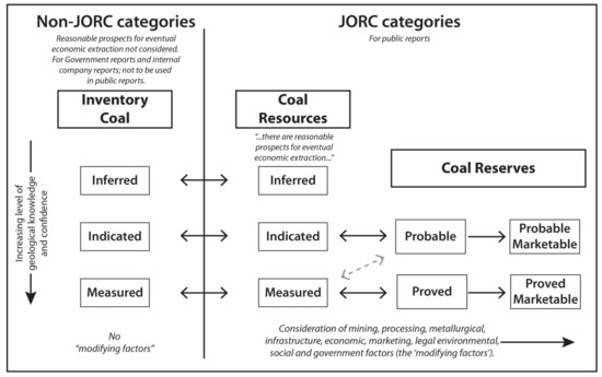
Figure 1.
The relationship between Inventory Coal, Coal Resource and Coal Reserves (modified from the Guidelines Review Committee [13]).
2.4.5. Exploration Results
If there is insufficient data to estimate a Mineral Resource (in the early exploration stage), then the Exploration Results (sampling intervals, grade, etc.) may be presented in a Public Report.
2.4.6. Exploration Target
A conceptual Exploration Target may be estimated in the early exploration stage. Both the quantity and the grade must be presented as ranges and it must be clear that the Exploration Target is a conceptual “order of magnitude” range of estimates.
2.4.7. Inferred Resource
The quality and quantity of an Inferred Resource are estimated from limited data, which is enough to imply, but not confirm, geological and quality continuity. Continuity cannot confidently be assumed.
2.4.8. Indicated Resource
An Indicated Mineral Resource quantity and quality are sufficiently delineated to be used (after appropriate adjustments from modifications from mining and processing the coal) as input into mine planning and economic evaluation. Continuity of coal can be assumed. A technical and economic study can be conducted at this stage, after which probable coal reserves can be publicly reported.
2.4.9. Measured Resource
A Measured Mineral Resource is estimated with enough confidence that it can be used as input into detailed mine planning and final evaluation of the economic viability. An estimation of either Probable or Proved Coal Reserves can then be publicly reported.
2.4.10. Inventory Coal
The term “Inventory Coal” is not covered by the JORC Code but was introduced in the Coal Guidelines [13]. It is coal that “can be estimated and reported without being constrained by economic potential.” Inventory Coal can also be subdivided into inferred, indicated, and measured sub-categories. Companies may be required to report Inventory Coal estimates to governments but cannot report these estimates publicly. If minimal exploration has been done, insufficient to establish even Inferred Resources, then the resource classification is not that of Inventory Coal, but an Exploration Target may be estimated.
Clearly, a company’s estimate of the coal resource may not be the entire quantity of interest to an assessment of the CSG potential of a deposit or region that has been explored for coal. Portions of a coal deposit may be too deep, the coal too thin, the quality too low, or the location too remote to make it of eventual economic interest. In addition, individual seams within an otherwise mineable sequence might be unmineable because of thickness, or perhaps because of many non-coal partings, but may still be of interest for CSG production.
With increasing limits on CO2 emissions, some thermal coal resources may over a 50-year period become uneconomic. Thus, some previous coal resource classifications may eventually be withdrawn, at which point the resource would be classified as Inventory Coal under the Coal Guidelines [13]. Inventory Coal might be of considerable interest as a CSG target, even though there are no reasonable prospects for mining.
2.4.11. Distance between Points of Observation
The JORC Code, being non-prescriptive, does not specify physical distances required between datum points for the varying resource sub-categories. Older versions of the Coal Guidelines [13] provided guidance. A previous edition of the Coal Guidelines in 2003 stated that Inferred Coal Resources (and Inferred Inventory Coal) may be estimated “using data obtained from Points of Observation up to 4 km apart.” To be assigned the status of “Indicated”, this distance was “normally less than 1 km apart,” with the qualification that it may be extended where justified, for example, by the use of geostatistical analysis. For Measured Coal Resources and Inventory Coal, this was “normally less than 500 m apart” with the same qualification about extending this if supported by geostatistical analysis. As pointed out by Larkin and Ballantine [16], all deposits are different and will therefore vary in the optimum spacing for each sub-category. In addition, of course, this is a level of guidance to the Competent Person that was not found in the original JORC Code, which relies heavily on the skills and experience of the Competent Person. The 2014 Coal Guidelines [13] removed a suggestion of maximum distances, firmly placing the responsibility for deciding the appropriate distance back on the Competent Person. Techniques to optimise the required spacing are mentioned by Larkin and Ballantine [16], including appropriate geological modelling and geostatistical analysis. These authors also point out that through the use of appropriate techniques the level of uncertainty may also be estimated, clarifying the degree of uncertainty for each sub-category as required by the JORC Code.
2.5. Classification of Coal Reserves
As defined by the JORC Code, an “Ore Reserve is the economically mineable part of a Measured and/or Indicated Mineral Resource.” An Ore Reserve (and therefore a Coal Reserve) is defined by pre-feasibility or feasibility studies. These studies may make allowances for “Modifying Factors”, including mining losses and addition of diluting materials (non-coal material not included in the resource estimate that will be added during the mining process). Any other “Modifying Factors” are also considered in converting resources to reserves.
2.5.1. Probable Coal Reserves
The relationship between Coal Reserves and Coal Resources is shown in Figure 1. Probable Coal Reserves is the economically mineable part of an Indicated Coal Resource, (or in some cases of a Measured Coal Resource) after completion of a technical and economic study that has identified the preferred mine plan, production schedule, and infrastructure.
2.5.2. Proved Coal Reserves
The confidence level of a Proved Coal Reserve is high. It is from the economically mineable part of a Measured Coal Resource after applying appropriate modifying factors. There must be high confidence in the geological, technical, and economic aspects of a Proved Coal Reserve, normally sufficient to allow an investment decision to be made. Discussion on the complete requirements to define a Proved Coal Reserve is of course provided in the relevant section of the JORC Code.
2.5.3. Marketable Coal—How Much of the Coal Reserve Will Be Sold?
Clauses 42 to 44 of the JORC Code [1] comprise a section termed “Reporting on Coal Resources and Reserves.” The term “Marketable Coal Reserves” is introduced, with the definition that this is the product after modifications due to mining, dilution, and processing have been considered. Much of the coal that is mined will also be processed, through a density separation process, to remove higher-density impurities. The product coal after processing is the Marketable Coal. The JORC Code states that “Marketable Coal Reserves must be reported together with, not instead of, reports of Coal Reserves.” The percentage of the original coal that remains after this separation is the yield. Any public report on Marketable Coal Reserves must include the amount of the predicted yield.
2.6. Coal Exploration Techniques
The estimation of coal resources follows a staged process with increasing geological confidence and reduced risk as the project progresses toward a decision to mine. At the time of the “Final Investment Decision” (FID) the geological risks are relatively low. As both thermal and coking coal are subject to sometimes-volatile price swings within price cycles, there remains market pricing risk, but this is mitigated by assessing the project’s investment returns throughout a price cycle, not by using temporary spot prices.
The initial exploration is done using relatively low-cost techniques as geological risk is high. With more certainty, exploration costs rise, and in the later years the exploration is combined with mining and marketing studies. The typical exploration techniques used at each stage are summarised by Edwards et al. [17]. Figure 2 illustrates typical stages of exploration activities in Indonesia, where there is often an emphasis on field mapping and outcrop sampling at preliminary stages of the programs [18]. More detail is given below.
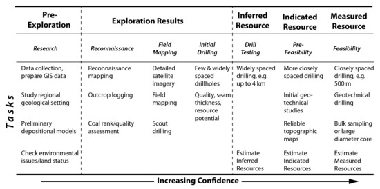
Figure 2.
Typical stages in exploration programs; note that this example was developed for Indonesian programs with their emphasis on field mapping and channel sampling of coal outcrops in the early stages of exploration (modified from Friederich [18]).
2.6.1. Research
The Research stage involves a compilation of all relevant data, including large-scale regional data sets, and starts with literature reviews. In Australia, this will include review of records from companies and state geological surveys that may have previously explored an area. Such data may not be freely available in other jurisdictions. The geological literature, including conference proceedings and research studies by post-graduate students, may also contain useful information. Understanding the geological setting, the location relative to markets and to known or potential infrastructure, and of course the target coal quality are important in generating an exploration target.
Data sets including open file regional geological maps and regional geophysical data and satellite imagery, are also important. In some situations, a company may choose to acquire its own airborne geophysical data over a prospective area.
2.6.2. Field Mapping
The importance of field mapping will vary. In some basins (e.g., in parts of Indonesia or New Zealand), many outcrops, particularly of coal, may be mapped along streams that cut through coal measures. A program of reasonably intensive field mapping along streams with channel sampling of coal intervals is an essential step before a more focused drilling program. Field mapping is low-cost and can be very effective, especially when combined with regional data such as satellite imagery.
2.6.3. Drilling
The first drilling program is usually widely spaced, targeting confirmation of coal thickness and coal quality and perhaps regional structure. Subsequent drilling programs become progressively more focused with reduced borehole spacing. Core recovery within coal seams must be high enough to ensure that the coal samples are representative of the seam. All boreholes, cored and non-cored, are downhole geophysically logged, a necessary step in confirming seam thickness and core recovery and allowing correlation of seams.
There are other exploration techniques that can be employed such as collection of coal samples for analyses, mapping of topography, geostatistical and geotechnical analysis, and seismic surveys. These and other techniques have been used previously [13,17].
2.7. Estimating the Coal Resources
After a sufficient level of exploration by cored drilling, infill non-cored drilling, and supplementary techniques such as field mapping and geophysical surveys, a geological model is created of the target coal seam(s). The amount of tonnes is then estimated by multiplying the area underlain by the coal of interest (square metres) by seam thickness (in metres) and the relative density; both thickness and density are estimated on a weighted average basis. Quality is also estimated on a weighted average basis. As noted in the Coal Guidelines [13], all coal quantities should be estimated at in situ moisture and relative density.
The steps involved in good practice in estimating coal resources are described in detail in the Coal Guidelines [13]. As noted, the seam distribution, depth, thickness, relative density, and moisture content are key points. Other quality parameters must also be assessed and reported. The estimation is supported by a detailed report and maps.
Individual coal seams must be correlated and the extent of any seam splitting defined. An intermediate step is to decide on the definition of “plies” within a seam (portions of a seam where the quality and thickness remain relatively persistent laterally) and to exclude thick non-coal partings that will definitely not be mined. The upper and lower seam boundaries are defined to develop a consistent “working section”, the interval that will probably be mined. The seams, their plies, and their splits are named individually so they can be modelled. This step is useful later in developing mine plans as it becomes easier to exclude marginal parts of the seam and to follow coal qualities and thicknesses across seam splits. At the end of this process the geological structure of the seam must be well understood. Once these steps have been conducted a computerised geological model can be generated.
Any geological model must take into account areas, identified by a geologist or a Competent Person, that are too thin or too deep or exceedingly structurally complex, which would preclude efficient mining. Once the model reliably represents the geology and quality of the coal seams then it can be used to generate weighted average properties.
The level of uncertainty within the model must also be understood. Possible areas of uncertainty, especially at the stage of estimating an Indicated Resource, might be the precise location of a major fault, the extent of intrusives impacting the coal seam, the extent of surface weathering near seam subcrop, or analytical uncertainty; for example, the true in situ moisture or quality variability. The JORC Code requires that areas of uncertainty be identified and discussed.
3. Classification of Coal Seam Gas from the Perspective of Petroleum
Compared to conventional petroleum systems, estimating the resources and reserves of gas in a coal seam is relatively new. Many of the methods of estimating gas volume had to be rethought for CSG reservoirs to be consistent with how the gas is stored within the coal (such as how the gas is held in pores). Pragmatic changes from conventional to CSG reservoirs when determining reserves also had to be adopted (for example, ultimate recovery could not be estimated until after de-watering, pressure draw-down, and then peak gas attained).
A CSG well profile is fundamentally different to that of conventional gas. In a conventional reservoir, such as sandstone, gas is produced immediately. The methane molecules are held within the pore spaces between the mineral grains. Once a conduit to the surface is made (e.g., a drillhole) gas buoyancy drives the molecules up the annulus to the surface. Once the greater volume of gas is removed from the reservoir, oil and then water, if present, will be produced (Figure 3A). In contrast, in a CSG reservoir, methane is attached to the sides of pores and thus it is the pore surface area, rather than the pore volume, as in conventional reservoirs, which is important [19,20,21,22,23]. Importantly, the methane molecules are held in place until the reservoir is de-pressurised, which means, in the case of CSG, that it is de-watered. Thus, a CSG play will show significant water production first, then once the reservoir is sufficiently de-pressurised gas will flow (Figure 3B). The time it takes to de-water and reach peak gas flow in a CSG play can vary greatly from days to months [21,24,25,26,27].
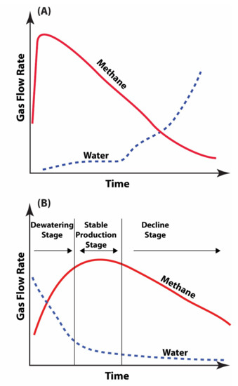
Figure 3.
Differences in production profiles from a (A) conventional natural gas well and (B) CSG well.
The purpose of this section is to set out how gas resources and reserves in CSG reservoirs may be estimated. At the risk of belabouring the point, but in the hope that clarity is achieved and expectations mitred, what is discussed is both directed only at CSG plays and is not meant to be exhaustive. That is, other practitioners may emphasize different aspects of estimating resources and reserves and still be within the confines of the guidelines. What is outlined, however, has been used repeatedly and successfully, with success being defined that the approach, as well as the results, have been acceptable (and in close approximation) to what other third-party certification companies have concluded from the same data. Additionally, the approach given here has been acceptable when submitted directly to various regulatory organisations.
Finally, although the PRMS, the COGEH, and the Chinese Standard are all discussed, it is only the PRMS that is covered in the most detail. Other articles, too, have discussed assessment methods of CSG and the reader is directed to Altowilib et al. [28], Boyer and Qingzhao [29], Chećko et al. [30], Jenkins and Boyer [31], Meneley et al. [32], Sarhosis et al. [33], Scott et al. [34], and Xia et al. [35].
3.1. Methods of Estimation
Most resource and reserve methodologies for petroleum allow for different types of determinations in both input variables (e.g., gas content) and data treatment to estimate a resource. For example, there are direct or indirect methods to determine the gas content of a reservoir. A direct method, for example, would be where gas content has been measured directly from a core [36,37,38,39,40,41,42] or from a flowing well. Data from direct methods can calculate resources volumetrically using a material balance approach or be gleaned from production performance data. The volumetric method, as the names implies, uses the volume and character of the reservoir, along with the gas content, to calculate gas in place. Material balance estimates of gas volumes use pressure data derived from the draw-down of wells, though this works best for higher-permeability reservoirs. Lower-permeability CSG reservoirs are not well suited for this type of resource analysis. Production performance of wells can also be used to estimate reservoir gas volume, but only after sufficient time has elapsed can reliable estimates be made.
An indirect method is when gas content measurements are extrapolated based on other known properties of the coal reservoir [39,42]. For example, if the rank, ash yield, and/or petrography are known for coal at a certain depth, then a range of gas contents can be projected using another coal reservoir where gas contents are known as an analogue. If maximum gas holding capacity has been measured (i.e., through an adsorption isotherm test [20,43,44,45,46]) on samples from a coal reservoir, but still no direct gas content measurements have been made, then actual gas content can be estimated by assigning a range of likely gas saturation values [21,47] from an analogue reservoir. Indirect (analogue) methods are usually only used during initial exploration phases where quite speculative resources are being estimated.
When all the variables needed to estimate a resource are assigned values [21,29,32,39,48], they can then be used either deterministically or probabilistically to estimate gas volume. A third method that uses geostatistical methods is also viable but is not discussed here. Probabilistic analysis takes the full range of all the individual input variables and randomly samples them using stochastic or Monte Carlo simulations [47,49,50,51,52,53,54,55]. Any probability level then can be used to estimate relative uncertainty. For example, a probability of 10% (P10) in most statistical probabilistic packages denotes a reasonable low end of estimates. What it means is that there is only a 10% chance that the “true” volume will be less than this value. A 90% probability (P90) is usually used as an upper, or high-end case value, while the 50% (P50) value is considered a base or best-case scenario. A P90 probabilistic value means that there is a 90% chance that the true volume is less than the estimate based on the input variables given. Interestingly, distinct from mathematicians and statisticians, the petroleum industry (including the PRMS) reverses the P10 and P90 definitions (so that the high-end case scenario, for example, is expressed as P10, meaning that there is a 10% chance that the actual quantities will exceed the estimate, while there is a 90% chance the actual value will be greater than the P90 estimate).
In a deterministic assessment the evaluator assigns a range of values for each variable, usually termed “high”, “base” (sometimes called “best”), and “low” cases. A base (or best) case is the one that the evaluator feels is most likely. The values chosen for high- and low-end scenarios are selected based on the evaluator’s experience and expertise and, unless there are other mitigating circumstances, roughly correspond, respectively, to what P10 and P90 (sensu PRMS) values might predict.
3.2. Petroleum Resource Management System (PRMS)
The Petroleum Resource Management System (PRMS) is the most widely used methodology for estimating CSG resources and reserves. This guideline is a joint collaboration between the Society of Petroleum Engineers (SPE), the American Association of Petroleum Geologists (AAPG), the World Petroleum Council, and other societies. Interestingly, although there are a number of industry publications (e.g., [56,57,58,59,60,61,62]) there are surprisingly few scholarly evaluation papers, though there are exceptions [51].
The purpose of the PRMS, as with any of the assessment guidelines, is to set out, as objectively as possible, standard procedures and terminology that clearly define the level of risk and uncertainty in any project at any particular time. Ultimately, the aim is to provide to potential investors (as well as regulatory and governance boards) a common set of rules and nomenclature for comparison of projects and their levels of uncertainty and risk. This discussion will focus on the criteria needed to gain different levels of resource or reserve designations. It is beyond the scope of the paper to delve into the detail of the PRMS and, thus, the reader is directed to the guidelines themselves for specifics. The most recent PRMS guidelines were published in 2018 [4], but the reader is directed to the extensive 2011 edition [3], which also has a subsection specifically on evaluating CSG reservoirs (written by industry experts Chris Clarkson and Geoffrey Barker).
The PRMS recognises that all geological, engineering, and economic variables have a range of uncertainty no matter how well known and characterised they may be. The PRMS therefore has been set out in such a way as to reflect both uncertainty as well as commercial risk. In the PRMS framework there are three main levels that are attributable to commercial risk and they are, in order of descending risk: Prospective Resources, Contingent Resources, and Reserves (Figure 4). Prospective Resources are considered “undiscovered”, while both Contingent Resources and Reserves are classed as “discovered”, although all three categories are simultaneously considered “recoverable”. This is an important distinction because of the significant increase in value that a deposit may have if it is designated as discovered.
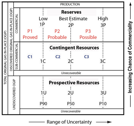
Figure 4.
Resource classification framework as defined by the Petroleum Resource Management System (PRMS) [4].
The horizontal axis of the PRMS framework is meant to show the degree of uncertainty at any of the resource or reserve levels. Some of the constraints on uncertainty for the different framework levels will be discussed below. But what all have in common is that, with a higher degree of characterisation, which is usually linked to having more data, the spread of possible values from high to low becomes more constrained. When there is little difference between high and low estimates there is more certainty. It must be said that it is not just about data quantity, but also quality. Analytical data that is obtained following well-established international or national standards will have higher confidence than unknown or little-used procedures. If it cannot be established which standards were used for which analyses, and/or the standards used are not recognised, then the analyses may be given large margins of errors, effectively increasing the level of uncertainty.
3.2.1. Prospective Resources
In a CSG play, Prospective Resources are assigned when the presence of coal reservoirs can be demonstrated. It is the easiest of the resource/reserve levels to attain and requires the least data and information. It is usually enough to show through outcrops of coal and/or subsurface drill wells or even the presence of mines that coal-bearing sediments occur. These types of data, even if sparse, establish if there is some continuity of the coal-bearing zone, though specific correlation of coal beds may not be possible. Gas content estimates are conducted either through analogy with other basins with similar-rank coal (thus, some coal quality data is required for Prospective Resource assignment) or if gas has been measured and documented in any nearby mines. It is not necessary to demonstrate that the gas is moveable; that is, no reservoir permeability tests need to be performed or gas saturation levels need to be determined for a deposit to be classed as a Prospective Resource. As noted previously, Prospective Resources are considered undiscovered petroleum initially-in-place (PIIP). A range of values that is designed to illustrate the level of uncertainty is also needed. A lower estimate of Prospective Resources (termed 1U) should correspond to having a 90% probabilistically determined chance that the actual quantities will exceed that estimate. The upper estimate (3U) corresponds to having only a 10% chance of being higher than the value. Finally, the intermediate value (2U) is equivalent to a 50% probability (which is the same as a statistical median value).
Note that Prospective Resources are usually reduced down from a calculated original gas in-place (OGIP) estimate. An OGIP will also have a range of values (low, best/base, high) like the Prospective Resources. The reduction from OGIP to Prospective Resources can vary greatly between fields or projects, largely a factor of what is determined to be unrecoverable versus recoverable. Resources may be unrecoverable for any number of reasons, including economic, technological, and sociological. At a later date, however, unrecoverable resources may become recoverable.
Finally, Prospective Resources may be reported on a “risked” or “unrisked” basis. Risk assessment is generally meant to encompass a determination of chance of commercial success. The PRMS is not prescriptive in what constitutes a commercial risk. However, it is noted that only the mean (P50) should have a risked success case. Contingent Resources are not risked in such a manner because, by definition, such an assessment is part of the criteria.
3.2.2. Contingent Resources
A Contingent Resource is one that has the potential to be recoverable, but at the time of assessment has not been deemed or demonstrated to be commercial. Commercial development of a resource could be contingent on a number of factors, including having a market or development of a key technology to assist deliverability or demonstration of a sufficiently large enough resource to be economic.
In order to be classed as a Contingent Resource, an area has to satisfy all the criteria for Prospective Resources plus have additional data. For CSG, the key additional data needed are:
- Core data with direct gas content (desorption) analyses which demonstrates a significant quantity of adsorbed gas, and
- Demonstration that the gas is moveable.
Although there are other possible methods to determine gas content [63], gas desorption from cores remains the most accepted and reliable.
Additional analyses, although not explicitly expected, can help to prove a Contingent Resource. Gas quality, that is, the relative proportion of CH4 to other gases, will demonstrate the value of a CSG play. A coal bed gas play that has high CO2 levels will be harder to develop. Another analysis that is helpful is an adsorption isotherm, which is conducted in the laboratory from a fresh sample of coal (preferably core) [21,44,46,64,65,66,67]. This test determines the maximum methane holding capacity of a sample of coal at different pressures under constant temperature. The test temperature used is usually the measured or estimated reservoir temperature at the depth the sample was collected.
The requirement to demonstrate that gas is moveable within in a CSG reservoir is perhaps open to interpretation, which may be why it is written as such. What this means, however, is that an operator needs to give some evidence that the gas, which is in the reservoir, can flow at a reasonable rate. The best and most direct way to demonstrate that gas in a coal reservoir is moveable, other than a flow test, is to conduct an in situ permeability analysis [68,69,70,71,72,73]. A less direct way to infer that hydrocarbons have the potential to be moveable is to determine gas saturation. The calculation of gas saturation requires that both adsorption and desorption isotherm analyses are conducted. Gas saturation is the difference between the maximum gas holding capacity (an adsorption analysis) at any given pressure (which means depth) and temperature and that of the actual gas charge (that is, the measured gas content from a desorption analysis) [21,25,74,75]. Even if a coal reservoir is highly permeable, if the gas saturation is low, gas flow may be negligible. Although there are a number of mitigating circumstances, gas saturations below 70% generally result in low gas flows, where peak flow is significantly delayed [26,27], and thus may be uneconomic.
Low permeability reservoirs may still be able to flow gas at reasonable rates if stimulated. However, a strong case needs to be made in order to satisfy the criteria that hydrocarbons are moveable within the reservoir. If the coal seam is at relatively shallow depths, depending on the initial measured permeability, then a case could be made that stimulation would result in economic gas flows. Basins with high horizontal stress, however, are problematic as artificially fractured coal reservoirs have a tendency to close up after initial fracture stimulation; even the use of proppant may not work on some coals because they will merely “close-up” around the grains.
Because of the importance of demonstrating the presence of moveable hydrocarbons in order to be classed as a Contingent Resource (and to be considered “discovered”) a short discussion of permeability is warranted.
Permeability is dynamic and changes with production. In general, permeability has a tendency to decrease as the reservoir is de-watered (which is necessary to release the gas) as a result of decreasing pore pressure, and with that decrease the cleat system closes up. In other words, after de-pressurising the reservoir, the formation water is no longer present to keep cleats and fractures open with the result that permeability decreases. However, through a process where the coal matrix shrinks as methane is removed [76,77,78,79,80,81], previously closed cleats re-open and permeability can then increase. The caveat here is if the gas saturation of a CSG reservoir is low then permeability may never recover [26,27]. Reservoirs with low permeability and low gas saturation may never have the ability to host “moveable” hydrocarbons. A final note on the dynamic nature of permeability in a CSG reservoir is that even in reservoirs where permeability does increase with production that increase may only be minimal. For example, some CSG production wells in the Bowen Basin, which began with an initial permeability of 1 mD, did increase but only to ~5 mD [81], and that increase is unlikely to produce substantial production.
The potential variability of permeability changes during production is one of the factors that drive uncertainty in a Contingent Resource assessment. The range of uncertainty is denoted at the low end as 1C, at the high end as 3C, and the base case is referred to as 2C. Note that 2C is the sum of both C1 and C2 portions of the estimate and, similarly, 3C is the sum of C1, C2, and C3 incremental volumes (Figure 4). The range of uncertainty can be determined using either probabilistic or deterministic methodologies.
Assigning a Contingent Resource requires making an estimate of the area that might be directly accessed by a production well. This is primarily accomplished through estimating the likely drainage area based on actual permeability measurements made in the reservoir or through an estimation based on an analogue. It must be recognised that not all the in-place gas resource can be recovered and a range of estimates must be made on how much can be recovered. Reservoir simulations can be used to estimate ultimate recovery (EUR). The final quantity of deliverable gas is influenced by a host of factors, including those already discussed as well as market pressures and influences.
Finally, although Contingent Resources can be assigned around single wells where gas content and an estimate of moveable gas has been made, if enough of these wells show consistent reservoir properties and chance of deliverability then areas between wells may also be classified as a Contingent Resource at some level (i.e., C1, C2, C3; Figure 4). This process is sometimes referred to as “rubber banding”.
3.2.3. Reserves
A Reserve designation under the PRMS is the highest rating given and indicates a high potential for commercial success. In the official definition, reserves must satisfy four criteria: they need to be “discovered”, recoverable, commercial and “remaining”. But to distil that down into very practical terms, the primary criterion to gain reserve status for a CSG play is to demonstrate that gas flow is economic. Although easily written, there is a lot in that short, simple statement. Firstly, sustained gas flow will need to be demonstrated over some period of time, ideally enough to reach peak production rate. This is particularly true in a new CSG field, where there are no other proximal producing neighbours. Secondly, and not as straight forward to demonstrate, is that any produced gas has to be commercially viable. This means several things all at once: there has to be a market for the gas, the price of the gas has to be higher than the cost of getting it out, and there has to be an intent for the deposit to be developed within a reasonable time frame (~5 years). Having a gas sales agreement (GSA) in place goes a long way toward demonstration of commerciality. There are exceptions of course and reserves may be designated from limited gas flow in a CSG well or even only from well data if a nearby field has a reasonable maturity.
Similar to the levels within the Prospective and Contingent Resources, a Reserve classification has three levels of certainty: Proved, Probable, and Possible. The Proved designation represents the least uncertainty and is the amount of gas that has been calculated to occur within the drainage area of a single currently producing well. A drainage area is that area where one well is thought to be able to drain within a reasonable timeframe. The size of the drainage area is essentially determined by the permeability of the reservoir at that area. A common grid used for Proved reserves in CSG is between 500 m to 750 m; this area is sometimes referred to as “Proved, Developed Producing” (or PDP). An additional “ring” of one drainage area in width can sometimes be assigned and is designated a “Proved, Undeveloped” (or PUD).
A Probable Reserve status indicates a higher degree of uncertainty of gas being present than that of the Proved Reserves. The actual area that a Probable Reserve would cover is largely dependent on the permeability of the reservoir; the more permeable the reservoir, the larger the drainage area. Additionally, if a CSG field is fairly mature and commerciality is well established, the area over which a Probable reserve could be claimed may be larger. Typically, though, two drainage units surrounding the Proved Reserve area are assigned (Figure 5).
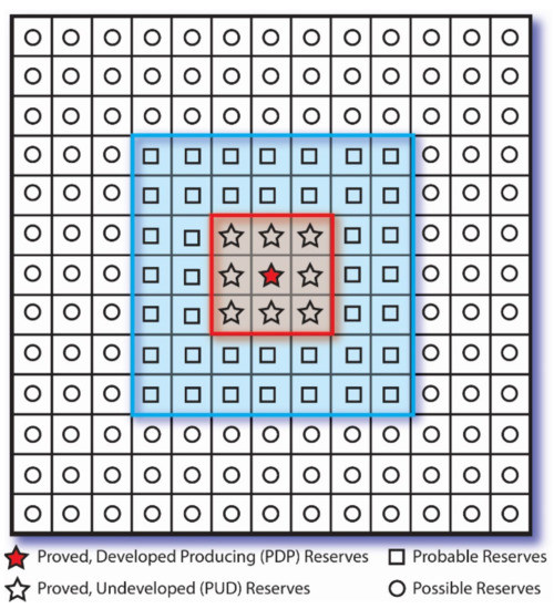
Figure 5.
Schematic of possible arrangement of Proved, Probable, and Possible Reserves based on a well drainage unit, represented here by individual squares. The size of each drainage unit will be determined by permeability and well type.
Possible Reserves are also concentrically assigned around the Probable Reserve. Although the area is usually three drainage units deep (Figure 5), that area may be increased or decreased primarily depending on the reservoir permeability and/or the overall field maturity. The Possible Reserves represent the least certain of the reserves.
Finally, 1P, 2P, and 3P designations represent the cumulative amount of gas reserves from the reasonably certain (1P = Proved), to the less certain (2P = Proved + Probable), and finally the even less certain (3P = Proved + Probable + Possible). In conventional reservoirs, it is the 1P volumes that are generally used to value a company, whereas for CSG it is the 2P reserves (cf. Figure 4).
Reserves in the PRMS can be calculated by a number of means; for example, through estimation of ultimately recoverable gas using history matching and future forecasting. The more production wells there are, generally the higher degree of confidence there is in making a best estimate of reserves. Whatever the methodology used, in a CSG reservoir a deterministic approach is often applied.
3.3. Canadian Oil and Gas Evaluation Handbook (COGEH)
The latest edition of the Canadian Oil and Gas Evaluation Handbook (COGEH) [5] is an impressive document. Previously, the COGEH was spread over three volumes all published and/or updated at different times: volume 1 in 2002 (with an update in 2007), volume 2 in 2005 (Resources Other Than Reserves, ROTR: 2014), and volume 3 from 2007–2014. The update consolidates those volumes into one document. Note that the COGEH is tied to the Canadian National Instrument 51–101 (NI 51–101), which is regulatory in nature and not discussed here.
The COGEH framework of resources and reserves is identical to that of the PRMS, which is not too surprising since the Society of Petroleum Evaluation Engineers (SPEE) was involved in both classifications. One of the most obvious differences, however, is that COGEH goes into a huge amount of detail defining almost every aspect of resource and reserve estimation, from resource classes to project description levels, from risk and uncertainty to reservoir simulation methods, as well as a plethora other attributes of assessment criteria. The COGEH also has an extensive section just on the estimation CSG. For a thorough understanding of hydrocarbon assessments, especially CSG, this is the document to consult. The biggest issue is that unlike the PRMS and Chinese Standard the COGEH is not freely available.
As a general rule, the COGEH is more specific about its requirements for attainment of different resource and reserve levels than the PRMS. For example, no reserves or resources (Contingent or Prospective) can be assigned on the basis of experimental technology. The COGEH is also explicit that a conservative (low) estimate for Prospective or Contingent Resources should be equivalent to a P90 probabilistic assessment, that an optimistic (high) estimate is to be equivalent to a P10 assessment, and finally a best (base) estimate should be close to a P50 probabilistic assessment.
Of particular note is that for Contingent Resources to be assigned in the COGEH there must be demonstrable coal within a 9.7 km radius and that there must be a reasonable expectation of production, which can be based on coal characteristics and the use of analogues. Importantly, any area assigned Contingent Resources must be bounded by data.
Finally, a significant difference between the COGEH and the PRMS are how reserves are treated. The COGEH has explicitly different criteria of assessment between Proved, Probable, and Possible Reserves. All Proved Reserves (Producing, Non-Producing, and Undeveloped) should have a probability equal to or greater than 90% (a conservative estimate), whereas Probable Reserves should be equivalent to a 50% probability and Possible Reserves have a probability equal to or greater than 10% (an optimistic estimate). The spacing assigned to any of the reserve classes is about 0.65 km2, and for Proved Reserves there has to be a producing well. Probable Reserves can only be assigned adjacent to a Proved area and where both the continuity of the coal seam and its properties are certain. For example, in areas where there are abundant faults or where the coal seam has a high rate of lateral thickness change, it may be difficult to assign Probable Reserves. For Possible Reserves, coal must be demonstrated to occur within a 3.2 km radius of a producing well or one that has had at least some tests confirming presence of gas that could be of economic producibility.
3.4. Chinese Standard
The Chinese Standard DZ/T 0216-2020 [6] for estimating the volume of gas in coal, by its own definition, can only be applied to “The hydrocarbon gas of which the main component is methane.” Furthermore, “coalbed methane resources” are defined as the “total amount of coalbed methane which occurs in a coal bed,” thus, by definition, it is important to remember that “coalbed methane” in the Chinese Standard is only that methane which is within the coal reservoir.
The Chinese Standard is structured differently than the PRMS and the COGEH standards. However, if the content and criteria are examined closely, the Chinese Standard is not that dissimilar in practise or intent. An important note is that the Chinese Standard uses the word “reserves” for almost everything, rather than reserves and resources as does the PRMS and the COGEH. The salient point is that at least some of what is referred to as “reserves” in the Chinese Standard should not be confused with how the PRMS or the COGEH use the designation “reserves”.
There are four basic categories in the Chinese Standard:
- Proved;
- Controlled;
- Inferred;
- Potential.
The Potential category is considered “to be discovered”, while the other categories are all classed as “discovered”. The difference between “discovered” and not yet discovered corresponds to the recoverability of the gas. An attempt has been made, as a visual aid, to show the interrelationships between the resource categories, commerciality, chance of success (“confidence coefficient”), and well type (Figure 6). It is recognised that not all the complexity of the Chinese Standard may have been captured in this figure.
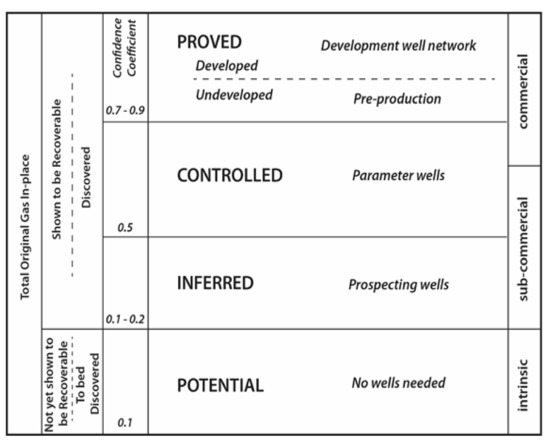
Figure 6.
Schematic of the classification framework for the Chinese Standard (DZ/T 0216-2020) [6].
The Potential Resources are the lowest designation and easiest to be assigned. These resources are obtained through analysis of regional geological information and/or analogy with other similar coal basins and no specific drill wells are needed. In other words, just the reasonable assurance that the presence of coal is in an area and some of its properties need to be demonstrated. The Chinese Standard also gives a “confidence coefficient” of 0.1. Which means there is only 10% confidence in this being a commercial CSG play. In the Chinese Standard it is described as having “intrinsic” commerciality, which means at the time of assessment, geological, economic, and technological uncertainty precludes any determination of whether the deposit is economic or not. This level would be roughly equivalent to Prospective Resources in the PRMS and the COGEH classifications.
The next level in the Chinese Standard is that of Inferred Resources. These are characterised through initial exploration efforts such as “prospecting” wells with cores that obtain coal quality, gas content, gas type, and other reservoir physical data. A regional analysis, which is required for Potential Resources, would also be needed. This level of resource has slightly higher confidence coefficients in the range of 0.1 to 0.2, i.e., 10–20% confidence that these deposits would be commercially extractable (Figure 6). Inferred resources are considered sub-commercial, which means that although at the time of the assessment, technical and economic conditions do not indicate economic benefits, a potential pathway may exist. Inferred Resources require gas data to be collected from core, but it does not have to be demonstrated that the gas is moveable. Thus, Inferred Resources in the Chinese Standard would be classed somewhere between Prospective and Contingent Resources in the PRMS and the COGEH classifications.
To be designated as a Controlled reserve in the Chinese Standard requires “parameter” wells to be drilled for all target layers. All analyses required for Inferred resources are also needed, plus permeability, gas saturation (i.e., both desorption and adsorption tests), and numerical simulation should also be conducted. The confidence coefficient for the data should be about 0.5 (or a 50% chance of being commercial). Controlled resources can be considered sub-commercial or commercial (Figure 6) l; the latter occurring if it can be demonstrated that development is technically feasible, economically reasonable, and with geological conditions that are not too complex. A business case has to be given that meets requirements for return on investment. This resource is most analogous to the Contingent Resource classification in the PRMS and the COGEH.
A Proved Reserve designation is the highest classification for a CSG deposit in the Chinese Standard and has the most stipulations it has to meet. To be classified as Proved requires all the analyses of the Controlled designation but with the addition of well tests that have a continuous 3-month production with all associated data. Well results must meet minimum production standards of 500 m3/day, 1000 m3/day, or 2000 m3/day for wells less than 500 m in depth, between 500 and 1000 m in depth, or >1000 m in depth, respectively. The confidence coefficient for data/results should be in the range of 0.7 to 0.9, that is, the results should indicate that there is a 70 to 90% chance of commercial success (Figure 6). Part of qualification of the designation of Proved is that its commerciality has been clearly demonstrated. This reserve grade in the Chinese Standard is most analogous to the Reserve class of the PRMS and the COGEH.
For Proved Reserves there is a secondary classification that relates to the areal extent that those reserves can be extended from a datum point. The well spacing requirements are divided into three groups based on geological (structural) complexity (Table 1). Category I is simple structures, such as gentle folds or monoclines; Category II is relatively complex geological structures such as folds, steep dips, and faults; Category III is complex geologic structure with compact (tight) folding and/or faulting or intrusives. Each of these categories are also further subdivided depending on variability of the coal bed thickness: Type 1 = coal thickness is stable throughout the area; Type 2 = coal thickness changes to a degree, but only slightly; Type 3 = coal thickness that is “instable”, that is, there is high variability in the lateral continuity of the seam from thinning and splitting. For the Controlled designation, well spacing cannot be more than two times the well spacing needed for Proved Reserves under the same structural and coal thickness variability conditions.

Table 1.
Well spacing requirements for different levels of geological complexity as indicated from the Chinese Standard.
Finally, reserves and resources can be estimated in the Chinese Standard through similar methodologies as prescribed for the PRMS and the COGEH classifications. Volumetric, analogy, and numerical simulations are all sanctioned as viable in the Chinese Standard.
3.5. Summary Comparison of the PRMS, the COGEH, and the Chinese Standard
Of the three classifications, the COGEH and the PRMS are most similar and use mostly the same criteria and terminology. The biggest difference between the two is that the COGEH is more specific in its requirements and less flexible in data types needed for various levels of resource assessment.
The Chinese Standard is more different from the PRMS and the COGEH than those two are to each other. But there are perhaps more similarities than real substantial differences between any of the classifications. The following is the basic framework that all of the schemes work within:
The lowest ranking resources (Prospective in the PRMS and the COGEH and Potential in the Chinese Standard) require only regional studies and demonstration that there is coal present with some knowledge of the coal rank and quality. These are termed “undiscovered”.
The highest-ranking resources (Contingent in the PRMS and the COGEH and Inferred to Controlled in the Chinese Standard) require a minimum of gas testing and collection of other reservoir properties, the most important of which is either permeability and/or gas saturation. These data need to demonstrate that there is potential to move economic quantities of gas. If this cannot be demonstrated (for example, if permeability or if gas saturation is low), then they cannot be classed as Contingent Resources. If data can demonstrate this possibility, then this would be termed “discovered”. The Chinese Standard has a slightly more nuanced classification in this regard in that the Controlled Reserves would definitely be equivalent to Contingent Resources, but the Inferred classification is somewhere between Prospective and Contingent.
The pinnacle of all three classifications is Reserves (or Proved reserves in the Chinese Standard). There is a very high standard for data before this classification can be applied to a gas deposit. The main criterion for this classification is commerciality. This is demonstrated through pilot or development wells. If a well does not reach commercial flows, then a reserve designation is highly unlikely to be given. This is especially true in green field basins where no previous CSG production has taken place.
The PRMS and the COGEH both have explicit methods to try and address uncertainty in estimates in all of the main layers of their system (i.e., Prospective, Contingent, and Reserves). A range of recoverable gas is given so as to give an indication of how certain the assessment is—a vital statistic for project and investment purposes. This uncertainty can be delineated deterministically or probabilistically. However, the Chinese Standard does not really have this in the same manner, and this constitutes the biggest divergence with the PRMS and the COGEH. Instead, the Chinese Standard takes into account geological complexity to help classify uncertainty. The geological complexity is denoted by two attributes: intensity of structural deformation and the degree of lateral variability of coal seam thickness. These are semi-quantitative, but they do act as a guide in assessing a field for further investment and management.
4. Differences and Similarities between the JORC Code and PRMS
4.1. Background—The Importance of Continuity of Coal Seams and Coal Quality
A resource estimate under the JORC Code requires consideration of the degree of continuity of geology and grade. In the context of coal, this is geological continuity of the relevant coal seams and continuity of the coal quality. Quantifying the degree of continuity within the JORC Code is defined as:
Inferred: The geological and quality continuity are implied but not verified.
Indicated: The exploration data are sufficiently detailed to assume geological and quality continuity.
Measured: The geological and quality continuity have been confirmed (Figure 7).
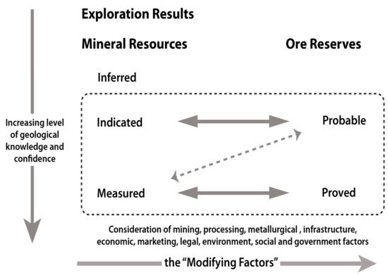
Figure 7.
The relationship between Exploration Results, Mineral Resources, and Ore Reserves [1].
In practice, this means that at the stage of estimation of measured resources, the location of faults is well defined, changes in seam thickness are understood, any seam splitting has been defined, and coal quality is well defined. Typically, in advanced projects, geostatistics may be completed to quantify variability of quality and seam thickness. For estimation of underground resources, seismic may be needed to better determine the extent and location of faulting that could disrupt underground mining. The presence of disruptive igneous intrusions or other discontinuities must also be determined. Of course, the distance between boreholes for each of these stages will vary between deposits depending on geological and quality complexity and, in some cases, depending on whether surface or underground mining is planned.
The need for this focus on continuity is clear. In the context of coal mining, any significant unexpected disruption in seam geology or coal quality could also significantly disrupt or delay mining and reduce the project’s economic value. For underground mining in particular, an unanticipated significant fault or intrusion could be disastrous to the value of a mine that uses capital intensive longwall techniques.
In the PRMS, as applied to CSG, less detail about continuity is needed than in the JORC Code. Production is from gas flowing to a well from the drainage area of that well. In that context, the drainage rates and gas volumes, as inferred from gas content and permeability tests and established by pilot wells, become more important than detail about the coal seam internal stratigraphy and its quality variations. Gas flow may in some circumstances be continued despite structural or geological changes that could wreak havoc on a mine plan. However, best practice still requires a good overall understanding of coal seam stratigraphy, geological structure, and the location of faulting. It is also important to understand the major quality parameters and broad scale variations, but of course not in the high level of detail required of coal mining by the markets that use the coal. Direct measurement of gas contents and saturation levels and flow rates is more important. Understanding continuity and coal quality is important in both the JORC Code and the PRMS, but it is the level of detail that differs significantly.
4.2. Similarities
Both the PRMS and JORC Code try to constrain uncertainty and risk and address commerciality through a classification system. Both are designed to give a more or less standardised system in which deposits can be characterized with the least ambiguity, primarily for investment purposes. Both the JORC Code and the PRMS have a three-tier system of classification comprised of:
- Preliminary data;
- Substantial data;
- Data that indicates commerciality.
Both classifications address the quality of product (whether coal or gas) as well as commerciality and uncertainty. In particular, the JORC Code addresses commerciality through:
- The criteria that a Mineral Resource must have “reasonable prospects for eventual economic extraction”, and
- The conversion from a Mineral Resource to an Ore Reserve through applying the Modifying Factors, essentially confirming commerciality through the confirmation of an Ore Reserve (see Figure 7); a final investment decision (FID) can be made at this time.
In addition, the JORC Code addresses resource estimate uncertainty through:
- The progression from an Exploration Result to a Mineral Resource,
- The progression from an Inferred Mineral Resource to a Measured Mineral Resource, and
- The increased certainty on the resource estimate needed for a Probable Reserve compared to a Proved Reserve, and greater clarity on the Modifying Factors.
For the PRMS, the three main tiers of classification (Prospective Resources, Contingent Resources, and Reserves (Figure 4)) define the level of data, and within each tier there is an assessment of uncertainty. The Reserves tier in both the PRMS and the JORC Code has to demonstrate a relatively high-level commerciality. In the JORC Code, a pre-feasibility or feasibility study is required as well as having a mine plan and planning for infrastructure, coal processing, a port, and estimates of markets and prices. It is very similar for reserves in the PRMS system, though for gas plants rather than coal, of course. Both systems must take into account the grade/quality and quantity of the product.
4.3. Differences
There is more emphasis in the JORC Code on the degree of continuity of the coal seam geology and quality of the deposit than in the PRMS. As a result, while the JORC Code and its Coal Guidelines are not prescriptive on borehole spacing, in practice a Competent Person would typically require a higher level of data than what is found in the PRMS, especially at the Coal Resource/Contingent Resource level. At the Coal Reserve/Gas Reserve level, the data density is more comparable, although there is still usually a higher data density for coal.
Another difference is that the JORC Code has only two reserve subclasses, while the PRMS has three. The JORC Code is more explicit in what parameters should be considered for commerciality than the PRMS, while the PRMS places less emphasis on a “Competent Person” doing the assessment than the JORC Code. Finally, there is less emphasis in the PRMS than the JORC Code on materiality and transparency.
5. Case Study: Resource Analysis Using the JORC Code and the PRMS
It was thought helpful to graphically demonstrate, in a hypothetical case study, the effect data types and geology may have on the determination of coal and CSG resources, reserves, and their distribution. The stratigraphic situation is given in Figure 8, and for this case study it can be assumed that coal and sediment thickness variations are relatively minor. Both hypothetical scenarios (i.e., coal and CSG) start with the constraints (i.e., town, national park), geological structure (i.e., faults, dipping strata), and data given in Figure 9.
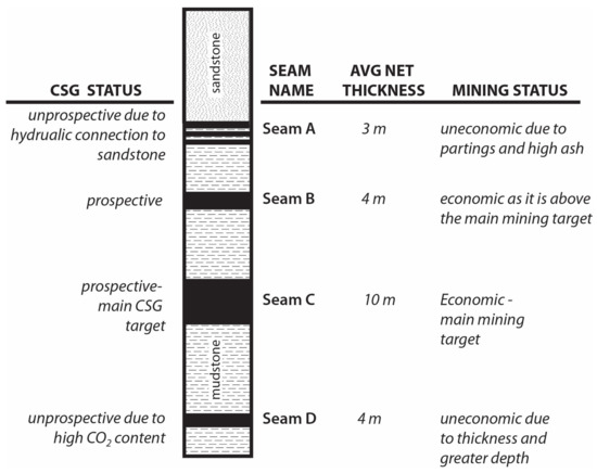
Figure 8.
Hypothetical vertical section showing stratigraphy and status relative to mining and CSG utilisation.
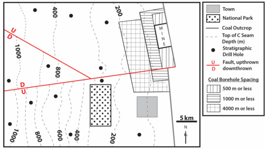
Figure 9.
Hypothetical case study showing boreholes, coal seam structure, and land use.
5.1. Coal Resources, Reserves, Exploration Targets, and Inventory Coal
The relevant figures illustrate a case study of a coal resource where both coal and CSG can be produced. There is a small operating mine on the eastern margin, in an area of shallow coal extending to the seam subcrop. There is a main target seam, Seam C, averaging 10 m thickness, with several other seams above and below it. Seam B, a 4-m thick seam, is economic for mining. Seam D is a 4-m thick seam that cannot be economically mined.
In addition, there is a town and a national park, both underlain by coal. In this scenario, for the purpose of this exercise, early coal exploration drilling in different times has extended to only 1 km north of the town (Figure 9). However, later discussions have come to mutual agreement that there will be a buffer zone of 5 km around the town, from which surface mining will be permanently excluded, and 2 km for underground mining. Mining and CSG production are of course excluded from below the National Park.
In this scenario, the most detailed exploration drilling, with a spacing of 500 m or less, was in the area of shallowest coal near the seam subcrop, north and south of the mine, aimed at determining whether the current small mine can be simply continued along strike (Figure 9). More widely spaced drilling, 1 km or less, has been conducted down dip in deeper coal to approximately 100 m depth. Drilling at a spacing of 4 km has been conducted to about 200 m depth, which informs the company and investors on the potential for a larger and deeper mine. (Note that these borehole spacings are illustrative only and are not intended as guidance for real projects!)
5.1.1. Exploration Target
Estimation of Exploration Targets is done relatively infrequently and typically at a very early stage in the exploration process and is meant to convey an “order of magnitude” assessment of the potential if exploration is successful. The estimation is included here as an illustration only and not to convey the methodology to be used. Often, exploration results will be presented instead without an estimate of the Exploration Target. An Exploration Target in this scenario would be mainly an underground target and would assume a high-quality coal. An Exploration Target was estimated only over areas not included within Coal Resources or Reserves (Figure 10). No estimate was made over the National Park or over the town and its exclusion zone. The result is expressed as a range of values. In this case, the upper range of underground coal thickness was decided as 10 m, extending down to 400 m depth of cover, over an area of 310 km2, or about 4090 million tonnes at relative density of 1.32. The lower range might be a mineable section of 4 m thickness, down to 300 m depth, over a smaller area of 234 km2, with 1390 million tonnes.
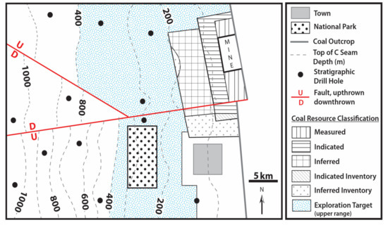
Figure 10.
Hypothetical case study showing coal resource distribution.
There is also an area of potentially surface mineable coal, in the north, where the upper range of thickness is 14 m (seams B and C) over an area of 35 km2, with an upper range estimate of 640 million tonnes. The lower range estimate is 370 million tonnes. The total estimate of both surface and underground potential is 4730 million tonnes (upper range) and 1760 million tonnes (lower range) (Table 2).
Table 2.
Results for hypothetical case study of tonnes of coal for different resource and reserve levels.
5.1.2. Coal Resources
Estimates of Coal Resources were made with classifications depending on the borehole spacing, as the assumption was made that this area was geologically not complex. The area of the Coal Resource estimates is shown in Figure 10.
Seam thickness was mostly 14 m (i.e., the combined thickness of seams B and C). The area of Measured Coal Resource was 25 km2, with a reduced coal thickness within a portion of this, outside the subcrop of Seam C. The area of Indicated Coal resource was 52 km2, and the area of Inferred Coal Resource was 78 km2.
5.1.3. Coal Reserves
Estimates of Proved Coal Reserves were made, with locations shown in Figure 11, within the area of Measured Coal Resources. As there were no complexities, the areas matched exactly. However, there were some coal losses in the mining process, resulting in a reserve estimate some 5% below the Measured Resource.
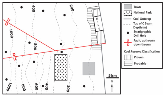
Figure 11.
Hypothetical case study showing coal reserve distribution.
The area of estimated Probable Coal Reserves broadly corresponds to the area of Indicated Resources (Figure 11). However, part of the Indicated Resources was excluded as the Probable Reserves are actually the area within a mine plan and part of the deeper coal had to be excluded. As a result, the area was reduced, to 41 km2 from 52 km2. The coal volume was further reduced 5% by mining losses.
5.1.4. Inventory Coal
The areas of Inventory Coal are shown in Figure 10. In this scenario, an area north of the town that had been explored in sufficient detail to allow an estimate of Indicated and Inferred Coal Resources was later excluded because of proximity to the town. A buffer of 5 km from the edge of the town was agreed. The Competent Person decided to also exclude a small part of the drilled area as it was regarded as too deep for surface mining. However, reporting to governments (e.g., to State Geological Surveys) typically requires reporting of all known coal volumes, whether economic or not. These volumes would be reported as Inventory Coal and are estimated in the same manner as Coal Resources.
5.2. Coal Seam Gas Resources and Reserves
Using the PRMS, one possible workflow scenario to derive original gas in place (OGIP), Prospective and Contingent Resources is given in Figure 12 and Figure 13. In step 1, all available data is assessed, including public and company data for the area in question. The target seams are identified, and, in this case, there are four (Figure 8). The important part in step 2 is determining what primary data there are to assess the coal seams, which includes coal thickness, distribution, and coal quality, especially ash content and relative density. In some cases, there may exist some reservoir data such as gas desorption, adsorption, or possibly permeability tests. If this is a CSG green field area, such as in our hypothetical case, there will be no gas data except, perhaps, for information that the local mine has gathered. In this case, we have access to the 12 stratigraphic drillholes as well as the high-density drilling associated with the mine (Figure 9). From this, we ascertain that there is little thickness variation in the possible CSG reservoirs. Since there are no reservoir data in the area, but we know the rank and coal quality with some certainty, we can use analogue data, such as gas content, quality, and saturation (step 3). Because we suspect that gas content will increase with depth, we take this into account. Finally, we know from the mine data that there is no indication of gas until depths of 75 m below the ground surface and thus shallower coal is not considered in this assessment.
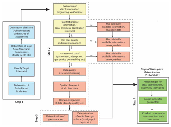
Figure 12.
One possible workflow scenario for determination of original gas in place (OGIP).
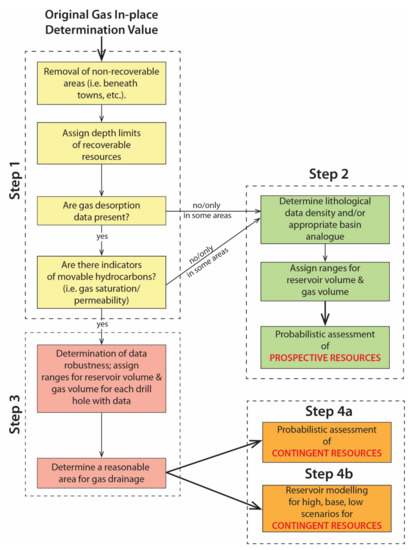
Figure 13.
One possible workflow scenario for determination of Prospective and Contingent Resources.
Since we only have basic coal thickness and depth and use analogue data for gas content, the OGIP will be determined probabilistically (Figure 14). Thus, ranges for each of the key variables (area, thickness, and gas content) for each coal seam (A-D) at different depths are assigned (step 4). In this hypothetical case, the resultant probabilistic assessment returns a P90 of 5,703 billion cubic feet (BCF; 162 billion cubic meters, BCM), a P10 of 6218 BCF (176 BCM), and a median (P50) of 5961 BCF (169 BCM) of gas (Figure 14A). Note that gas volumes of resources and reserves are given only as a guide for scale and trends.
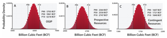
Figure 14.
Probabilistic distribution for (A) original gas in place (OGIP), (B) Prospective Resources, and (C) Contingent Resources in the hypothetical case study area.
The determination of OGIP usually does not use any, or possibly only a few, mitigating factors when determining gas volumes. However, when Prospective and Contingent Resources are determined, assessments must take into consideration the potential for recoverability. Thus, in the hypothetical case study presented here, for the Prospective Resource assessment we must remove areas that are known (or very highly likely) not to be accessible for gas drainage, such as towns and national parks (Figure 13). Although analogue data is still fine to use for a Prospective Resource assessment, a range of possible recoverability factors will need to be given. Typically, recoverability factors will be higher in shallower reservoirs and decrease with depth. In this example, recoverability has been given a range of 40–65% for the shallower depths of each seam, while a lower and wider range of 25–60% were used for the deeper, lower permeability reservoirs. The higher range of recoverability at greater depth is to reflect the increase in uncertainty. The area of Prospective Resources is shown in Figure 15A, noting that both the national park and the relevant proportion of the town have also been removed. A probabilistic analysis results in a P90 of 2364 BCF (67 BCM), a P10 of 2747 BCF (78 BCM), and a median (P50) of 2550 BCF (72 BCM) of gas (Figure 14B) when all seams and depth ranges are taken into account.
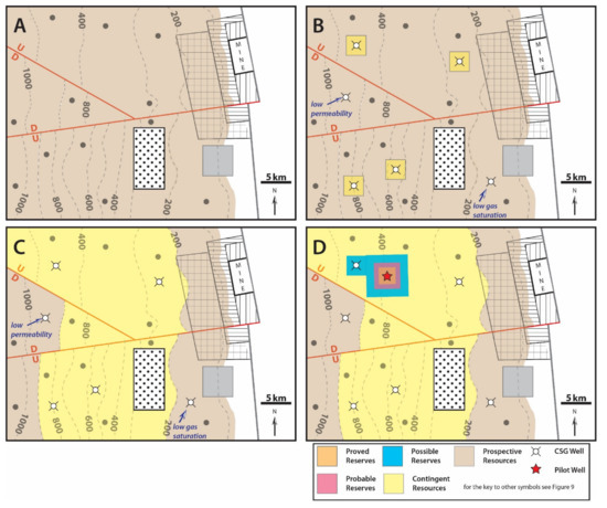
Figure 15.
Hypothetical case study showing distribution of (A) Prospective Resources, (B) initial assignment of Contingent Resources, (C) full extent of Contingent Resource after “rubber banding”, and (D) Reserves distribution after a successful pilot well.
To achieve the next level of resource classification (Contingent) in the hypothetical case given here, six wells were drilled, and all seams received desorption, adsorption, gas quality, and coal quality tests. Wells were also tested for permeability. Note that in real situations wells drilled to collect core can often be problematic to then test for permeability. In many of the wells, seam A was found to be in hydraulic connection with the overlying sandstone, which is deemed a regional aquifer. Thus, seam A cannot be developed at this time and is not considered as a Contingent Resource. In addition, seam D was found to have high levels of CO2 in most of the wells and would be considered uneconomic and therefore also cannot be considered as a Contingent Resource. Seams B and C, however had good gas contents, quality, saturation and permeability in four of the six wells. Those four wells have been given a designation of Contingent Resource in a 3 × 3 km area around the drillhole (Figure 15B). In the well that targeted seams at 950 m the permeability was very low and thus not considered to be able to produce movable gas. Although the well at about 180 m had good permeability, the gas saturation was so low that movable gas will not occur and thus cannot be given a Contingent Resource designation. In this hypothetical case study, this is considered enough data to “rubber band” the Contingent Resource areas for seams B and C between the depths of 200 m and 900 m (Figure 15C). A probabilistic assessment was conducted on this large Contingent Resource area. In our hypothetical case study, the drilling found that the gas contents in seam B were slightly lower but slightly higher in seam C than what was used previously from analogue data. Thus, the gas content ranges have been updated to reflect the new, site-specific data. In addition, because permeability and gas saturation in these depths were favourable, the recoverability factor has been increased, though still is higher at shallower depths and lower in deeper areas. The resultant analysis then indicates that the P90 Contingent Resources are 1607 BCF (46 BCM), with a P10 of 1840 BCF (52 BCM) and a P50 of 1721 BCF (49 BCM) (Figure 14C).
Finally, in the hypothetical case study, a pilot well is drilled (Figure 15D). The well was allowed to flow long enough to de-water the reservoir and reach peak gas. During this time the nearby CSG well was monitored for reservoir connectivity, which showed a strong response and suggested an optimal drainage area per well of about 700 m2. Using history matching and forecast modelling, an estimated ultimate recovery (EUR) per well drainage area has been determined to be 0.42 BCF (0.12 BCM). In this case study, the company has been able to demonstrate that the gas is of economic value in terms of markets, infrastructure, and requisite governmental permits. Thus, reserves have been awarded and estimated deterministically based on drainage area and the pilot well production. A Proved Reserve of 3.78 BCF (1.07 BCM) has been determined with 0.42 BCF (0.12 BCM) of that being Proved, Developed and Producing (PDP) and 3.36 BCF being Proved, Undeveloped (PUD). Probable Reserves have been estimated at 16.8 BCF (4.76 BCM). Because of the proximity and demonstration of connectedness between the pilot well and the nearby CSG well, an area surrounding that well has also been awarded Possible Reserves, which in combination with the pilot well results in a total of 54.18 BCF (15.34 BCM). Thus, the uncertainty in reserves can be expressed as ranging from 3.78 BCF (1P; 1.07 BCM) to 20.58 BCF (2P; 5.82 BCM) to 74.76 BCF (3P; 21.17 BCM). These values, though not derived from a probabilistic analysis, would be equivalent to P90 (conservative estimate), P50 (best case), and P10 (an optimistic estimate).
6. Summary
Gas extraction and mining of coal can occur coevally or sequentially and, thus, it is an advantage to understand how each is quantified. In this paper, we have reviewed the salient attributes of the main classification system for coal (the JORC Code) and CSG (the PRMS). In addition, the COGEH and the Chinese Standard for assessing CSG has also been compared with the PRMS. In summary we have found:
- All classification systems allow resources to be classed based on the level of data collected, and this is related directly both to uncertainty and commercial risk,
- The highest classification levels are reserves in all systems, though the criteria to attain them can be different between coal (the JORC Code) and gas (PRMS, COGEH, Chinese Standard),
- In general, the JORC Code is more stringent in its requirements (through the Competent Person) on borehole density for resources or reserves at any particular level,
- The PRMS and the Chinese Standard place less emphasis on the role of a “Competent Person” than the COGEH, while the JORC Code places the most emphasis,
- The COGEH tends to be more prescriptive and descriptive about requirements to attain different levels of resources as well as reserves than the PRMS or the Chinese Standard,
- Both the PRMS and the COGEH give substantial detail about how to quantitatively assess uncertainty statistically,
- The Chinese Standard is the most explicit in identifying geological structure and coal reservoir character in defining risk, which impacts on resource and reservoir level, and
- Finally, in a hypothetical case study using the same initial data, the JORC Code and PRMS had overlapping, though not necessarily aligned, resource and reserve designations.
Author Contributions
Both authors contributed equally in the conceptualisation, direction and conclusions of the paper. M.C.F. wrote mostly on the coal resource and reserve assessments while T.A.M. wrote mostly on the coal seam gas resource and reserve assessments. All authors have read and agreed to the published version of the manuscript.
Funding
The writing of this paper received no external funding.
Institutional Review Board Statement
Not applicable.
Informed Consent Statement
Not applicable.
Data Availability Statement
Not applicable.
Acknowledgments
Both authors wish to acknowledge the input of the three anonymous reviewers who helped to improve the manuscript. T.A.M. wishes to acknowledge the direct, hands-on, practical learning of resource estimation he has gained while in the employment of such companies as Solid Energy NZ, Arrow Energy International, Sinopec Oil and Gas Australia, and Origin Energy as well as the numerous other companies he has consulted to, including Ephindo Energy, Exxaro, Vale, ExxonMobil, Sugico Energy, PetroChina, Strike Energy, Sucofindo, Dart Energy, and others. The analysis of a diverse range of coals in basins throughout the world illustrates how important data, context, and geology is to any resource assessment. M.C.F. acknowledges the leading role of the Australian Institute of Mining and Metallurgy (AusIMM) and related professional groups in developing, then promoting to their membership and to industry stakeholders, an understanding of the benefits of a systematic code for public reporting of mineral resources and reserves, and for the educational resources provided for their members. He also wishes to acknowledge both the formal training and the practical learning of resource estimation and of applying the relevant codes while employed by BHP Billiton and by other companies that he has worked for or consulted to in coal basins in a wide range of geological settings.
Conflicts of Interest
The authors declare no conflict of interests.
References
- Joint Ore Reserves Committee (JORC). Australasian Code for Reporting Exploration Results, Mineral Resources and Reserves; Australasian Institute of Mining and Metallurgy, Australian Institute of Geoscientists and Minerals Council of Australia: Melbourne, VIC, Australia, 2012; 44p. [Google Scholar]
- Society of Petroleum Engineers. Petroleum Resources Management System; Society for Petroleum Engineers: Houston, TX, USA, 2007; 47p. [Google Scholar]
- Society of Petroleum Engineers. Guidelines for Application of the Petroleum Resources Management System; Society of Petroleum Engineers: Richardson, TX, USA, 2011; 221p. [Google Scholar]
- Society of Petroleum Engineers. Petroleum Resources Management System; Society of Petroleum Engineers: Richardson, TX, USA, 2018; 57p. [Google Scholar]
- Society of Petroleum Evaluation Engineers. Canadian Oil and Gas Evaluation Handbook, 3rd ed.; Society of Petroleum Evaluation Engineers: Calgary, AB, Canada, 2020; 460p. [Google Scholar]
- Ministry of Natural Resources of the People’s Republic of China. Regulation of Coalbed Methane Reserves Estimation, DZ/T 0216-2020; Ministry of Natural Resources of the People’s Republic of China: Beijing, China, 2020; 20p. [Google Scholar]
- Schmoker, J.W. Resource-assessment perspectives for unconventional gas systems. AAPG Bull. 2002, 86, 1993–1999. [Google Scholar]
- Schmoker, J.W. U.S. Geological Survey assessment concepts and model for continuous petroleum accumulations. In Total Petroleum System and Assessment of Coalbed Gas in the Powder River Basin Province, Wyoming and Montana; U.S. Geological Survey Digital Data Series-69-C, Chapter 4, CD-ROM Version 1; USGS Powder River Basin Province Assessment Team, Ed.; U.S. Geological Survey: Reston, VA, USA, 2004. [Google Scholar]
- Wood, G.H.; Kehn, T.M.; Carter, M.D.; Culbertson, W.C. Coal Resource Classification System of the U.S. Geological Survey; Geological Survey Circular 891; U.S. Geological Survey: Reston, VA, USA, 1983; 65p. [Google Scholar]
- Miskelly, N.; West, R. The Australasian Joint Ore Reserves Code in Practice. In Proceedings of the The AusIMM Annual Conference, Perth, Australia, 24–28 March 1996; pp. 313–316. [Google Scholar]
- Coombes, J. Refining competent persons criteria for resource geologists. In Proceedings of the Ninth International Mining Geology Conference, Adelaide, Australia, 18–20 August 2014; pp. 153–158. [Google Scholar]
- Stephenson, P.; Miskelly, N. Reporting standards and the JORC Code. In Mineral Resource and Ore Reserve Estimation—The AusIMM Guide to Good Practice; The Australasian Institute of Mining and Metallurgy: Melbourne, Australia, 2001; pp. 653–661. [Google Scholar]
- Guidelines Review Committee. Australian Guidelines for the Estimation and Classification of Coal Resources; Coalfields Geology Council of New South Wales and the Queensland Resources Council: Maitland, NSW, Australia, 2014; 47p. [Google Scholar]
- Davis, M.; Radonich, A. Unreasonable Prospects: What Does 50 Years in Coal Mining Actually Mean? In Proceedings of the Bowen Basin and Beyond, Bowen Basin Symposium 2015, Brisbane, QLD, Australia, 7–9 October 2015; Beeston, J.W., Ed.; The Bowen Basin Geologists Group and the Geological Society of Australia Incorporated Coal Geology Group: Sydney, Australia, 2015; pp. 253–266. [Google Scholar]
- International Energy Agency (IEA). Net Zero by 2050. A Roadmap for the Global Energy Sector; IEA: Paris, France, 2021; 222p, Available online: https://iea.blob.core.windows.net/assets/beceb956-0dcf-4d73-89fe-1310e3046d68/NetZeroby2050-ARoadmapfortheGlobalEnergySector_CORR.pdf (accessed on 23 July 2021).
- Larkin, B.; Ballantine, G. Classification of an example coal resource using conditional simulation. In Proceedings of the Bowen Basin and Beyong, Bowen Basin Symposium 2015 Brisbane, QLD, Australia 7–9 October 2015; Beeston, J.W., Ed.; The Bowen Basin Geologists Group and the Geological Society of Australia Incorporated Coal Geology Group: Sydney, Australia, 2015; pp. 267–274. [Google Scholar]
- Edwards, J.; Barlett, K.; Hatherly, P.; Lea, J.; Wilson, F.G. Exploration of deposits. In Australasian Coal Mining Practice, Monograph 12, 3rd ed.; The Australasian Institute of Mining and Metallurgy: Melbourne, Australia, 2009; pp. 93–111. [Google Scholar]
- Friederich, M.C. Coal Exploration Techniques and Reporting (Presentation); Seminar on Professional Reporting on Exploration Results and Resource/Reserve Estimates; MGEI and IAGI: Bandung, Indonesia, 2009. [Google Scholar]
- Gürdal, G.; Yalçin, M.N. Pore volume and surface area of the Carboniferous coals from the Zonguldak basin (NW Turkey) and their variations with rank and maceral composition. Int. J. Coal Geol. 2001, 48, 133–144. [Google Scholar] [CrossRef]
- Li, Q.; Liu, D.; Cai, Y.; Zhou, Y.; Yin, T. Investigation on the methane adsorption capacity in coals: Considerations from nanopores by multifractal analysis. Energy Fuels 2021, in press. [Google Scholar] [CrossRef]
- Moore, T.A. Coalbed methane: A review. Int. J. Coal Geol. 2012, 101, 36–81. [Google Scholar] [CrossRef]
- Şenel, I.G.; Gürüz, A.G.; Yücel, H. Characterization of pore structure of Turkish coals. Energy Fuels 2001, 15, 331–338. [Google Scholar] [CrossRef]
- Yu, S.; Bo, J.; Liu, J.-G. Nanopore structural characteristics and their impact on methane adsorption and diffusion in low to medium tectonically deformed coals: Case study in the Huaibei coal field. Energy Fuels 2017, 31, 6711–6723. [Google Scholar] [CrossRef]
- Kang, J.; Fu, X.; Gao, L.; Liang, S. Production profile characteristics of a large dip angle coal reservoir and its impact on coalbed methane production: A case study on the Fukang west block, southern Junggar Basin, China. J. Pet. Eng. Technol. 2018, 171, 99–114. [Google Scholar] [CrossRef]
- Moore, T.A.; Zarrouk, S.J. The origin and significance of gas saturation in coalbed methane plays: Implications for Indonesia. In Proceedings of the Indonesian Petroleum Association, Thirty-Fifth Annual Convention & Exhibition, Paper IPA11-G-195, Jakarta, Indonesia, 18–20 May 2011; Indonesian Petroleum Association: Jakarta, Indonesia, 2011; 10p. [Google Scholar]
- Wang, X.J. Influence of Coal Quality Factors on Seam Permeability Associated with Coalbed Methane Production. Ph.D. Thesis, University of New South Wales, Sydney, Australia, 2006. [Google Scholar]
- Zheng, A.; Wang, X.; Wang, X.; Wu, M.; Yuan, Y. The effect of coal seam gas saturation on CBM well productivity—A case study of central region of Hedong area. Procedia Eng. 2011, 26, 1205–1213. [Google Scholar] [CrossRef] [Green Version]
- Altowilib, A.; AlSaihati, A.; Alhamood, H.; Alafnan, S.; Alarifi, S. Reserves estimation for coalbed methane reservoirs: A review. Sustainability 2020, 12, 10621. [Google Scholar] [CrossRef]
- Boyer, C.M., II; Qingzhao, B. Methodology of coalbed methane resource assessment. Int. J. Coal Geol. 1998, 35, 349–368. [Google Scholar] [CrossRef]
- Chećko, J.; Howaniec, N.; Paradowski, K.; Smolinski, A. Gas migration in the aspect of safety in the areas of mines selected for closure. Resources 2021, 10, 73. [Google Scholar] [CrossRef]
- Jenkins, C.D.; Boyer, C.M., II. Coalbed- and shale-gas reservoirs. J. Pet. Eng. 2008, 60, 92–99. [Google Scholar]
- Meneley, R.A.; Calverley, A.E.; Logan, K.G.; Proctor, R.M. Resource assessment methodologies: Current status and future direction. AAPG Bull. 2003, 87, 535–540. [Google Scholar] [CrossRef]
- Sarhosis, V.; Jaya, A.A.; Thomas, H.R. Economic modelling for coal bed methane production and electricity generation from deep virgin coal seams. Energy 2016, 107, 580–594. [Google Scholar] [CrossRef] [Green Version]
- Scott, A.R.; Zhou, N.; Levine, J.R. A modified approach to estimating coal and coal gas resources: Example from the Sand Wash Basin, Colorado. AAPG Bull. 1995, 79, 1320–1336. [Google Scholar]
- Xia, L.; Yin, Y.; Yu, X.; Zheng, Y. An approach to grading coalbed methane resources in China for the purpose of implementing a differential production subsidy. Pet. Sci. 2019, 16, 447–457. [Google Scholar] [CrossRef] [Green Version]
- Bertard, C.; Bruyet, B.; Gunther, J. Determination of desorbable gas concentration coal (direct method). Int. J. Rock Mech. Min. Sci. 1970, 7, 43–65. [Google Scholar] [CrossRef]
- Diamond, W.P.; Levine, J.R. Direct Method Determination of the Gas Content of Coal: Procedures and Results; Report of Investigations 8515; U.S. Bureau of Mines: Washington, DC, USA, 1981; 36p. [Google Scholar]
- Diamond, W.P.; Schatzel, S.J. Measuring the gas content of coal: A review. Int. J. Coal Geol. 1998, 35, 311–331. [Google Scholar] [CrossRef]
- Mavor, M.; Nelson, C. Coalbed Reservoir Gas-In-Place Analysis; GRI-97/0263; Gas Research Institute: Chicago, IL, USA, 1997. [Google Scholar]
- McCulloch, C.M.; Levine, J.R.; Kissell, F.N.; Deul, M. Measuring the Methane Content of Bituminous Coalbeds; Report of Investigations 8043; US Bureau of Mines: Washington, DC, USA, 1975; 22p. [Google Scholar]
- Smith, D.M.; Williams, F.L. Direct method of determining the methane content of coal—A modification. Fuel 1984, 63, 425–427. [Google Scholar] [CrossRef]
- Williams, R.J.; Yurakov, E. Improved Application of Gas Reservoir Parameters; Wollongong, ACARP Project No C10008 (GeoGAS report 2003-244); GeoGas Pty Ltd.: Mackay, Australia, 2003; 111p. [Google Scholar]
- Bustin, R.M.; Clarkson, C.R. Geological controls on coalbed methane reservoir capacity and gas content. Int. J. Coal Geol. 1998, 38, 3–26. [Google Scholar] [CrossRef]
- Crosdale, P.J.; Moore, T.A.; Mares, T.E. Influence of moisture content and temperature on methane adsorption isotherm analysis for coals from a low-rank, biogenically-sourced gas reservoir. Int. J. Coal Geol. 2008, 76, 166–174. [Google Scholar] [CrossRef]
- Laxminarayana, C.; Crosdale, P.J. Controls on methane sorption capacity of Indian coals. AAPG Bull. 2002, 86, 201–212. [Google Scholar]
- Yee, D.; Seidle, J.P.; Hanson, W.B. Gas sorption on coal and measurement of gas content. In Hydrocarbons from Coal; Law, B.E., Rice, D.D., Eds.; Studies in Geology 38; American Association of Petroleum Geologists: Tulsa, Oklahoma, 1993; pp. 203–218. [Google Scholar]
- Moore, T.A.; Mares, T.E.; Moore, C.R. Assessing uncertainty of coalbed methane resources. In Proceedings of the Indonesian Petroleum Association, 33rd Annual Convention & Exhibition, IPA09-G-056, Jakarta, Indonesia, 5–7 May 2009. [Google Scholar]
- Bustin, R.M.; Bustin, A.M.M. Horseshoe Canyon and Belly River coal measures, south central Alberta: Part 1—Total original gas-in-place. Bull. Can. Pet. Geol. 2011, 59, 207–234. [Google Scholar] [CrossRef]
- Chen, Y.; Yang, Y.; Luo, Y. Uncertainty analysis of coalbed methane economic assessment with Monte Carlo method. Procedia Environ. Sci. 2012, 12, 640–645. [Google Scholar] [CrossRef] [Green Version]
- Crovelli, R.A. Probabilistic assessment methodology for continous-type petroleum accumulations. Int. J. Coal Geol. 2003, 56, 45–48. [Google Scholar] [CrossRef]
- Khisamov, R.S.; Safarov, A.F.; Kalimullin, A.M.; Dryagalkina, A.A. Probabilistic-statistical estimation of reserves and resources according to the international classification SPE-PRMS. Georesources 2018, 30, 158–164. [Google Scholar] [CrossRef]
- Mehana, M.; Callard, J.; Kang, Q.; Viswanathan, H. Monte Carlo simulation and production analysis for ultimate recovery estimatino of shale wells. J. Nat. Gas Sci. Eng. 2020, 83, 103584. [Google Scholar] [CrossRef]
- Moore, T.A.; Friederich, M.C. A probabilistic approach to estimation of coalbed methane resources for Kalimantan, Indonesia. In Kalimantan Coal and Mineral Resources; Basuki, N.I., Prihatmoko, S., Eds.; MGEI-IAGI Seminar: Balikpapan, Indonesia, 2010; pp. 61–71. [Google Scholar]
- Yang, Y.; Chen, Y.; Qin, Y.; Cheng, Q. Monte-Carlo method for coalbed methane resource assessment in key coal mining areas of China. J. China Univ. Geosci. 2008, 19, 429–435. [Google Scholar]
- Zuber, M.D. The use of Monte Carlo analysis to evaluate prospective coalbed methane properties. In Coalbed Methane: Scientific, Environmental and Economic Evaluation; Mastalerz, M., Glikson, M., Golding, S.D., Eds.; Kluwer Academic Publishers: Dordrecht, The Netherlands, 1999; pp. 55–66. [Google Scholar]
- Barker, G.J. Application of the PRMS to coal seam gas. In Proceedings of the 2008 Asia Pacific Oil & Gas Conference Adn Exhibition, SPE Paper 117124. Perth, Australia, 20–22 October 2008. [Google Scholar]
- Carpenter, C. PRMS classifications: A new methodology for resource inventory management. J. Pet. Technol. 2019, 71, 50–51. [Google Scholar] [CrossRef]
- Chan, P.B.; Etherington, J.R.; Aguilera, R. Using the SPE/WPC/AAPG/SPEE/SEG PRMS To Evaluate Unconventional Resources. SPE Econ. Manag. 2012, 4, 119–127. [Google Scholar] [CrossRef]
- Cronquist, C. Estimation and Classification of Reserves of Crude Oil, Natural Gas, and Condensate; Society of Petroleum Engineers: Richardson, TX, USA, 2001; 416p. [Google Scholar]
- DiLuzio, D. An update of the global standard in reserves/resources classification and definitions. J. Pet. Technol. 2018, 70, 74–77. [Google Scholar] [CrossRef]
- Kreft, E.; Godderij, R.; Scheffers, B. The value added of five years SPE-PRMS. In Proceedings of the SPE Annual Technical Conference and Exhibition, Amsterdam, The Netherlands, 27–29 October 2014; Society of Petroleum Engineers: Richardson, TX, USA, 2014; 10p. [Google Scholar]
- Macdonald, D.; Falcone, G.; Heiberg, S.; Ross, J.; Griffiths, C.; Denelle, F.; Coll, C. UNFC: Expanding the Influence of PRMS beyond Petroleum; SPE-181623-MS; Society of Petroleum Engineers: Richardson, TX, USA, 2016; 9p. [Google Scholar]
- Lamarre, R.A.; Pope, J. Critical-gas-content technology provides coalbed-methane-reservoir data. J. Pet. Technol. 2007, 59, 108–113. [Google Scholar] [CrossRef]
- Crosdale, P.J.; Beamish, B.B.; Valix, M. Coalbed methane sorption related to coal composition. Int. J. Coal Geol. 1998, 35, 147–158. [Google Scholar] [CrossRef]
- Crosdale, P.J.; Saghafi, A.; Williams, R.; Yurakov, E. Inter-laboratory comparative CH4 isotherm measurement on Australian coals. In Proceedings of the Bowen Basin Symposium 2005, Yeppon, QLD, Australia, 12–14 October 2005; Beeston, J.W., Ed.; The Geological society of Australia: Sydney, Australia, 2005; pp. 273–277. [Google Scholar]
- Karacan, C.O.; Okandan, E. Adsorption and gas transport in coal microstructure: Investigation and evaluation by quantitative X-ray CT imaging. Fuel 2001, 80, 509–520. [Google Scholar] [CrossRef]
- Zhou, Y.; Zhou, L. Fundamentals of high pressure adsorption. Langmuir 2009, 25, 13461–13466. [Google Scholar] [CrossRef] [PubMed]
- Clarkson, C.R.; Bustin, R.M. Coalbed methane: Current field-based evaluation methods. SPE Reserv. Eval. Eng. 2011, 14, 60–75. [Google Scholar] [CrossRef]
- Kamenar, A.; Taco, G.; Edgoose, J. How to plan a safe and successful permeability program in coal seams. In Proceedings of the 17th Coal Operator’s Conference, Mining Engineering, University of Wollongong, Wollongong, Australia, 8–10 February 2017; pp. 341–349. [Google Scholar]
- Ramurthy, M.; Marjerisson, D.M.; Daves, S.B. Diagnostic fracture injection test in coals to determine pore pressure and permeability. In Proceedings of the SPE Gase Technology Symposium, Calgary, AB, Canada, 30 April–2 May 2002; Society of Petroleum Engineers: Richardson, TX, USA, 2002; 16p. [Google Scholar]
- Salmachi, A.; Dunlop, E.; Rajabi, M.; Yarmohammadtooski, Z.; Begg, S. Investigation of permeability change in ultradeep coal seams using time-lapse pressure transient analysis: A pilot project in the Cooper Basin, Australia. AAPG Bull. 2019, 103, 91–107. [Google Scholar] [CrossRef]
- Wang, X.; Wu, Q. Methodology review of interpreting permeability of CBM reservoir across Asia Pacific region. In Proceedings of the The 3rd Asia Pacific Coalbed Methane Symposium, Paper No. 091. Brisbane, Australia, 3–6 May 2011. [Google Scholar]
- Zhou, F.; Yao, G. Sensitivity analysis in permeability estimation using logging and injection-falloff test data for an anthracite coalbed methane reservoir in Southeast Qinshui Basin, China. Int. J. Coal Geol. 2014, 131, 41–51. [Google Scholar] [CrossRef]
- Mares, T.E.; Moore, T.A.; Moore, C.R. Uncertainty of gas saturation estimates in a subbituminous coal seam. Int. J. Coal Geol. 2009, 77, 320–327. [Google Scholar] [CrossRef]
- Pashin, J.C. Variable gas saturation in coalbed methane reservoirs of the Black Warrior Basin: Implications for exploration and production. Int. J. Coal Geol. 2010, 82, 135–146. [Google Scholar] [CrossRef]
- Connell, L.D. A new interpretation of the response of coal permeability to changes in pore pressure, stress and matrix shrinkage. Int. J. Coal Geol. 2016, 162, 169–182. [Google Scholar] [CrossRef]
- Connell, L.D.; Mazumder, S.; Sander, R.; Camilleri, M.; Pan, Z.; Heryanto, D. Laboratory characterisation of coal matrix shrinkage, cleat compressibility and the geomechanical properties of determining reservoir permeability. Fuel 2016, 165, 499–512. [Google Scholar] [CrossRef]
- Durucan, S.; Ahsan, M.; Shi, J.-Q. Matrix shrinkage and swelling characteristics of European coals. Energy Procedia 2009, 1, 3055–3062. [Google Scholar] [CrossRef] [Green Version]
- Gray, I. Reservoir engineering in coal seams: Part 1. The physical process of gas storage and movement in coal seams. SPE Reserv. Eng. 1987, 2, 28–34. [Google Scholar] [CrossRef]
- Levine, J.R. Model study of the influence of matrix shrinkage on absolute permeability of coal bed reservoirs. In Coalbed Methane and Coal Geology; Special Publication No. 109; Gayer, R., Harris, I., Eds.; The Geological Society: London, UK, 1996; pp. 197–212. [Google Scholar]
- Mazumder, S.; Scott, M.; Jiang, J. Permeability increase in Bowen Basin coal as a result of matrix shrinkage during primary depletion. Int. J. Coal Geol. 2012, 96–97, 109–119. [Google Scholar] [CrossRef]
Publisher’s Note: MDPI stays neutral with regard to jurisdictional claims in published maps and institutional affiliations. |
© 2021 by the authors. Licensee MDPI, Basel, Switzerland. This article is an open access article distributed under the terms and conditions of the Creative Commons Attribution (CC BY) license (https://creativecommons.org/licenses/by/4.0/).