Review

The Influence of Outdoor Particulate Matter PM2.5 on Indoor Air Quality: The Implementation of a New Assessment Method

by
Dominik Bekierski
* and
Krystyna Barbara Kostyrko
Thermal Physics, Acoustics and Environment Department, Building Research Institute (ITB), 1 Filtrowa Str., 00-611 Warsaw, Poland
*
Author to whom correspondence should be addressed.
Energies 2021, 14(19), 6230; https://doi.org/10.3390/en14196230
Submission received: 5 August 2021 / Revised: 14 September 2021 / Accepted: 22 September 2021 / Published: 30 September 2021
(This article belongs to the Special Issue Energy Efficiency and Indoor Environment Quality)

Abstract

:
Epidemiological research has shown that there is a positive correlation between the incidence of disease and mortality in humans and the mass concentration of particulate matter. An average 1 g of suspended dust emitted in a room results in the same exposure as 1 kg emitted to the outside air. In this study, the authors described the state of knowledge on dust pollution inside and outside buildings (I/O ratios), and methods of testing the PM infiltration process parameters. According to the law of indoor–outdoor particle mass balance and the physical basis of aerosol penetration theory, a relatively simple but new method for estimating the penetration factor P was tested. On the basis of the curve of dynamic changes of internal dust concentration in the process of particle concentration decay and next of the followed curve of dynamic rebound of particle concentration, authors measured penetration factor of ambient PM2.5 through building envelope. Authors modification of the method is to be used for determining the value of the particle deposition rate k not from the course of the characteristics in the transient state (the so-called particle concentration decay curves) but from the concentration rebound course, stimulated by natural particle infiltration process. Recognition measurements of the mass concentration of suspended PM2.5 and PM10 particles inside the rooms were carried out. In this study, the choice of the prediction particle penetration factor P calculation method was supported by the exemplary calculation of the p value for a room polluted by PM2.5. The preliminary results of the penetration factors determined by this method P = 0.61 are consistent with the P factor values from the literature obtained so far for this dimensional group of dusts.

1. Introduction

The aim of the article is to present the authors’ proposal for a new method of assessment of the influence of outdoor particulate matter PM2.5 on indoor air quality indirectly by determining the value of the parameter that determines the intensity of dust penetration into the interior of the building. This parameter is the penetration factor, i.e., the ratio of the amount of dust entering from the outside, ending the infiltration processes, to the amount of dust retained outside.
In this study, the authors described the state of knowledge concerning dust pollution inside and outside buildings (I/O ratios), and methods of testing the PM infiltration process parameters. Methods known in the literature are based on the observation of the process of dynamic air pumping from a dusty external environment into a room with the use of an exhaust blower or an air cleaner. However, the process is not only dependent on the difference in PM concentration levels but more on the O/I air pressure difference produced. The authors’ proposal includes the observation of the PM concentration rebound curve of the dust indoor concentration level increasing caused by the natural process of dust infiltration from the outside, to achieve dust balance in the exterior and interior of the building protected by a dust-permeable envelope.
The authors’ field study aimed to estimate indoor air quality, especially particulate matter concentration in relation to the infiltration process through the buildings’ envelope. Several analyses based on air quality measurements and calculation procedures were undertaken. On the basis of the curves of dynamic changes of internal dust concentration in the processes of particle concentration decay and next followed curves of dynamic change particle concentration rebound the authors proposed the method of estimating the value of the penetration factor of ambient PM2.5 through a building envelope. Information on the value of the P factor can be a reliable parameter that classifies buildings in terms of resistance to dust infiltration into their interior, which partly characterizes the condition of the envelope structure and its resistance to dust penetration into the building. According to research in residential buildings, a large proportion of both groups of particles and their mass concentration are attributed to human activities such as cooking, smoking, vacuuming, gas stoves, the burning of solid fuels and candles, electrical appliances, cleaning, washing and walking. Both sources influence the characteristics of indoor particulate matter, and their concentrations are increased by the resuspension of particles deposited on internal surfaces in the air.
The term PM10 is used for particles with an aerodynamic diameter <10 µm. The term PM2.5 defines aerodynamic particles with a diameter <2.5 μm. The coarse fraction contains particles with an aerodynamic diameter between 2.5 µm and 10 µm. The “ultrafine particles” fraction has an aerodynamic diameter <0.1 µm. A commonly used indicator describing particulate pollution is the mass concentration of PM10.
Thatcher and Layton’s [1] experiments concluded that PM > 5 µm may be resuspended, particles < 5 µm are not easily resuspended and particles < 1 µm show almost no tendency to re-suspend at high human activity.
In the project INDEX PM [2], it was demonstrated that indoor air PM dust pollution mainly consists of salt (ammonium sulphate, ammonium nitrate, sodium and potassium chloride), soot (elemental carbon, EC), minerals (silicon oxides, aluminium, calcium, iron, manganese, titanium, zinc, etc.), organic substances (shredded organic matter, also called organic carbon, OC) and materials of biological origin (bacteria and fungi, dandruff, pollen, fragments of plants and insects). All of these components have different particle size distributions and mechanisms, which are strongly dependent on particle size and are involved in removing particles from the indoor air. Sedimentation is the most important mechanism for the removal of coarse particles (>10 μm), diffusion and the agglomeration/coagulation of ultrafine particles (<0.1 μm).
Particles (0.1–1.0 μm) are most stable in air. A typical input fraction (fraction of the total PM mass emitted from the source that will be inhaled by the whole population) for an indoor PM source is 10−2 to 10−3, compared to 10−5 to 10−6 for outdoor PM sources: An average 1g of suspended dust emitted in a room results in the same exposure as 1kg emitted to the outside air. Consequently, while internal sources are less efficient and their total emission loads are smaller than the PM of external sources, each of these sources, if present, may dominate both the sum of individual exposures and the inhalation risks of PM.
Between 1999 and 2016, the Canadian Census Health and Environment Cohort (Can-CHEC) conducted panel studies involving approximately 2.5 million Canadians [3]. The relationship between non-accidental mortality and the concentration of fine particulate matter (≤2.5 μm; PM2.5), ozone (O3) and nitrogen dioxide (NO2) in the environment was investigated. Models with combinations of these contaminants have also been tested and PM2.5 was found to be associated with an increased risk of non-accidental mortality, i.e., lung cancer, diabetes and ischemic heart disease. The results obtained provide evidence that long-term exposure to these three key components of ambient air pollution is associated with an increased risk of non-accidental mortality. Cumulative risk models suggest that exposure to PM2.5 alone does not fully characterise the toxicity of a mixed atmosphere and cannot fully explain the mortality risks associated with exposure to environmental contamination. The strongest cumulative risk estimate is for mortality from diabetes (HR = 1.180; 95% CI: 1.125, 1.236). Assuming the additive exposure of individual pollutants, HR (Health Risk) in 95% CI (Confidence Interval), as estimated using three pollutant models showed that a change in exposure by an average of 5% for all three pollutants together resulted in impact synergies of 1.075. The effect of PM2.5 and O3 was weaker than the effect of NO2 alone, but HR increased with the combination of all three pollutants, i.e., adding NO2.
It has also been proved that the strongest correlation between PM2.5 concentration and mortality increased by 1.5% when PM2.5 concentration increased by 10 μg/m3 per day [3], because particulate matter <PM2.5 enters into the bloodstream.
The health effects of PM2.5 were also studied by Hvelplund [4]. The Brownian motion of particles in the respiratory system is only visible for particles below 0.05 µm. The same tendency was found by Wang et al. [5], who investigated the deposition efficiency of particles with aerodynamic diameters between 0.001 and 300 µm moving through the nasal cavity with an air mass flow of 0.6 m3/h. Studies in this area have shown that the lowest deposition efficiency is in the range of 0.015 to 10.0 µm due to the low influence of diffusion and the effects of impact and gravity settling.
The number of exhaled particles is debatable, e.g., most particles below 1.0 µm were predicted to escape through the bronchiolar orifices. It is not the case, however, that all particles escape because some of them are absorbed directly into the bloodstream through the bronchioles, which in human airways make up most of the levels of the tracheobronchial tree. Particles larger than 5–10 µm are usually removed from the upper respiratory tract, indicating that the mucosa and nasal hair contribute greatly to the filtration of particles.
According to [4], inhalation exposure to particulate pollutants is one of the main threats to public health. Most existing airway morphometry models are theoretical or semi-empirical in nature; they were designed to predict the deposition fraction for an averaged subgroup of the general population. It is difficult to tailor a quick and accurate prediction to suit individual needs.
Hvelplund et al. [4] aimed to analyse the local particle deposition along an anatomically reconstructed model of the airways, which was developed from computed tomography images of healthy subjects. Computational simulations of airway fluid dynamics show that most particles are deposited in the bronchi. The accumulation of particles (0.1–2.0 µm) is the smallest fraction, about 11%, of sediment in the lower respiratory tract. Increasing the aerodynamic diameter >2.0 µm of the particles increased the fraction of deposited particles. This study determined the size related to the site of particle deposition in the airways. It turned out that most of the particles in the studied bands are deposited in a narrow region of the airway model, such as the BC (bronchi) and larynx.
Already in the 1980s, many epidemiological studies had shown that PM2.5 has obvious side effects on human health Lin et al. [6]. Research in China on the relationship between PM2.5 and human health has fully demonstrated that PM2.5 can increase the incidence of heart and lung disease, respiratory disease, cardiovascular disease, cancer and other diseases, and even the risk of death. Long-term exposure to environmental PM2.5 may be an important risk factor for hypertension and is responsible for the significant burden of hypertension in adults in China, as it leads to a reduction in lung function. PM2.5 is a risk factor for childhood asthma, attributed to decreased immunoregulation and deterioration in ventilation function. Exposure to PM2.5 can also affect reproductive health.
The I/O indicator describing the temporary steady state of dust pollution in a building is related to the process of infiltration of suspended dust from the outside into the building’s interior and can be described with the assumption that there are no internal sources generating dust particles:
I O r a t i o = C i n C o u t
Lee et al. [7] found that room temperature and floor level (expressed by the story where the room is located in the building) are powerful I/O predictors and gave the I/O equation for PM2.5, which is:
I O = 0.629 + 0.0102 · T 0.00654 · F L  
where T and FL are temperature and floor level, respectively.
The indoor/outdoor (I/O) index is a measure for assessing the difference between the levels of indoor solid concentrations and the current outdoor concentrations, but it may be also recognised as an indicator of the persistence of particulate matter sources inside buildings.PM concentrations are affected by dust infiltration from the outside into buildings and internal sources. I/O ratios can vary considerably due to the building’s design, location and the different activities of the occupants. The I/O ratio is also calculated to compare the dynamics of flows between indoor and outdoor PM in different apartments and buildings. As far as health protection is concerned, it is clearly the best when the I/O ratio for each dimensional fraction of dust is less than 1, asthisshows that the structural properties of a residential building reduce the penetration of PM from outside and, accordingly, reduce the residents’ exposure to PM.
In epidemiological studies of external contamination, the concentration of external contaminants was previously used as an indicator of the stressor. Thus, the appropriateness of using suspended dust concentrations from the building surroundings as a proxy in personal exposure studies was questioned, and both outdoor and indoor concentrations began to be measured to investigate their correlation with external conditions, as well as the correlations among other pollutants. Positive correlations were found for PM, O3 and NO2.
While exposure to indoor air pollution changes under the influence of many factors, such as the type of microenvironment and the source of internal pollution, building characteristics and its location, ventilation parameters and assumed comfort conditions (Branco et al. [8]), as well as individual building occupant activity, studies have shown that only some of these factors are important. Therefore, several parameters of I/O interaction (Kalimeri et al. [9])were selected in order to minimise the error resulting from the use of concentrations in the external environment as a surrogate for estimating the exposure of the PM environment to humans indoors. These parameters are the infiltration coefficient (Finf) (i.e., the equilibrium fraction of particles from the environment that have penetrated into the interior and remain suspended), the P coefficient of penetration efficiency of particles through the leaks of the building envelope (i.e., the fraction of particles that entered the interior from the infiltration path through the external walls of the building, P < Finf) and the I/O ratio (the ratio of internal to external concentration of similar PM particles). Lv et al. [10] argued that regression analyses of the ratio of inside and outside particle concentration values confirm that the degree of correlation of changes in these concentrations expresses the infiltration coefficient.
Nadali et al. [11] found that coarse particles, e.g., PM10, have higher falling velocities than fine PM, which leads to lower levels in rooms, because coarse particles (PM) settle under the influence of gravity or settle on doors, window frames and furniture as a result of the effects of electric charges and turbulent diffusion.
In their research, the concentration of solid particles, expressed by the average I/O ratio, also differed significantly in apartments, and did not solely depend on the location of the buildings. This was because, although the air with PM outside can have a significant impact on the concentrations inside, the composition of the air in the room is mostly influenced by the sources (activities and materials) in the rooms, which can be identified as contributing significantly to the internal mass concentration of PM.
Bai et al. [12] addressed the question why the I/O ratio is so important in practice. Everyday health is characterised by the equation of health detriment for each individual, based on an environmental risk assessment from the “receptor” perspective of
H H D i , j i n h a l a t i o n = C i , j · ( I R × t j m ) · E F
where C is the concentration of particulate matter (μg/m3) with the indices: i = spring or summer or autumn or winter (1:1:1:1 annually), j = inside or outside (ratio 80:20), HHD is damage to human health t is the daily exposure time h, m is an I/O mixing ratio of 1, EF is an influence factor of 78 DALY/kg (or disease cases/kg of chemical intake), IR is the daily inhalation rate of air for each person, which is 13/24 (m3/h).
In questionnaire studies [12], the daily ratio of the students’ exposure time to air polluted with dust inside and outside was calculated, and the mixing coefficient m was determined (the same as the I/O ratio). Due to different daily PM2.5 concentrations, health effects at different concentrations were calculated from Equation (3). The daily damage to the health of each person multiplied by the period of a year is the annual damage to the health of one person.

2. The State of Knowledge on Dust Pollution Inside and Outside Buildings

2.1. Characteristics of Actual Air Pollutants in the Internal Environment

According to the European programme INDEX-PM [2], the indoor air sources of PM are classified as:
  • PM from external sources transferred to the premises via ventilated or infiltrated air;
  • PM from external sources, transferred to the premises as settled dust and then re-suspended in the air in the room;
  • suspended dust from indoor combustion sources, such as tobacco smoke, cooking, candles or forest fires;
  • particles of biological origin; and finally;
  • particulate matter produced by indoor air chemistry, e.g., oxidation of cleaning ingredients (e.g., terpenes) by ozone.
Zhang and Duan [13] showed that burning a mosquito on a heating coil can release 626 µg/m3 PM2.5, which is 8.3 times the permissible concentration for a residential environment. Bai et al. [12] examined the concentration of PM2.5 in households using coal for cooking and found that it was significantly higher than in households using gas or electricity, and if coal was switched to gas or electricity, the concentration of PM2.5 in the kitchen would decrease by 40–70%. Zhang et al. [14] investigated different culinary habits, cooking methods, ingredients and even spices and found that they strongly influenced the composition of particulates. Culinary habits were also the subject of research by another group of researchers, Xue, Zhou et al. [15], who warn against the residential combustion of coal with a high sulphur content, as it can cause the total concentration of air pollutants to contain as much as 11.6% PM10 and even 27.5% SO2 in the winter heating season.Zhou, Liu. [16] indicated that human activities such as walking, dressing and cleaning may increase the concentration of PM2.5 indoors by 33%. Chinese researchers conducted experiments on the influence of wet sweeping and dry sweeping in the air in an office. The average levels of PM2.5 concentrations in the rooms before cleaning were 47.3 µg/m3, 40.6 µg/m3 and 39.4 µg/m3, respectively. The average levels of PM2.5 concentrations inside the premises after cleaning were 109.7 µg/m3, 97.5 µg/m3 and 43.3 µg/m3, respectively. The mean concentrations of PM2.5 increased 2.3 times, 2.3 times and 1.1 times, respectively. Therefore, it is recommended to wet sweep as often as possible under ventilation conditions. Printing also plays a role in increasing indoor dust concentration, and the release of PM2.5 from printers with different performance varied.
Some systematisation of the main sources of indoor air pollutants in our living environment is a necessary step to facing and reducing the associated health risks. Three different environments are described: Home, school and office, and the pollutants for the home, including particulate matter, are listed in Table 1. These were data published at the Healthy Building conference by Simeone et al. [17] supplemented by data from the literature.
According to Wallace and Ott [20], cooking on gas or electric stoves and electric toaster ovens was a major source of UFP, with peak personal exposures often exceeding 100,000 particles/cm3 and estimated emission rates in the neighbourhood of 1012 particles/min.
He, Morawska and Gilbert [25] investigated submicrometric particle number concentration measured during the cooking test and found that it was in the size range from 0.015 to 0.685 µm.
Jantunen [18], in a study with multiple regression models using data collected from the EXPOLIS from six European cities, determined the internal concentrations of PM2.5, starting from the concentration generated by smoking (16%), a gas cooker (1.4%), construction dust and a gas cooker (all < 4%).Smoking and cooking also generated NO2 emissions. The research focused on the short-term effects of internal sources of PM, which are, e.g., different cooking methods generating concentrations of various solid particles in rooms, with peak concentrations of 30–60 μg/m3 for PM0.02–0.5 and 10–300 μg/m3 for PM0.7–10. Cleaning activities (8 μg/m3 for PM0.02–0.5 and 30 μg/m3 for PM0.7–10) and those related to the mobility of residents (4 μg/m3for PM0.02–0.5 and 20 μg/m3 for PM0.7–10) contributed much less. Oven roasting was the most intense source of PM0.5 indoors, as well as frying (PM10).
Morawska et al. [26] report that some types of activity of inhabitants result in particularly high concentrations of PM2.5 in rooms. These include frying (median peak value: 745 μg/m3), grilling (718 µg/m3), candle evaporating eucalyptus oil (132 µg/m3) and smoking (79 μg/m3). The high maximum concentrations caused by these activities may result in the US EPA PM2.5 standard being exceeded for 24 h at 65 μg/m3 in homes where such activities are carried out, provided that the activity is carried out for more than 24 h.
The reported emission rate of 0.99 mg/min−1 from smoking is comparable with the results reported in the literature. For example, Klepeis et al. [27] measured the emissions factor of the respirable particle (PM3.5) emitted in an apartment where smoking took place. It turned out that the average PM3.5 emission index ranged from 0.98 mg/min−1 (cigar) to1.9 mg/min−1 (Marlboro cigarette). Brauer et al. [28] measured cigarette smoking using a nephelometer positioned in an environmental chamber and found that the emission rate of PM2.5 particles was 1.67 mg/min−1.
In a US indoor/outdoor air study, it was determined that smoking and cooking were the predominant activities associated with an elevated concentration of “fine particles”. Smoking can add 20 µg/m−3 (24 h average) of particles per household smoker [29] with short-term peaks of 300 µg/m−3 that may persist for up to 30 min after the cigarette is extinguished. Home cooking generated particles (0.1 µm) accounted for 30% of the particle volume [30]. The cooking method, and particularly frying, variably increased particle concentration, and the consensus states that the I/O ratios were somewhat higher in houses with gas cookers than in houses without such cookers and heating sources. Large particles (>2.5 µm in diameter) are generated in homes with activities such as home cleaning (vacuuming and sweeping) [30,31], which can lead to the re-suspension of particles embedded in horizontal surfaces such as floors, carpets and furniture. The ratio between indoor and outdoor particle concentrations gives an indication of whether particles found indoors are the result of indoor generation.

2.2. Limit Values for Indoor PM Concentrations

The data taken from the Health-Based Ventilation Guidelines: Principles and Framework, which were published in [32,33], can be considered as setting the latest limit values for the exposure of humans to indoor pollutants, see Table 2 The guidelines adopted the data from the WHO Air Quality Guidelines, Global Update 2005 published in 2006 by the Regional Office for Europe (Copenhagen) [34] concerning the most life-threatening pollutants NO2, PM10, PM2.5 and O3, but also SO2, considered by some researchers to be an equally hazardous pollutant.

2.3. Characteristics of Actual Air Pollutants in the Outdoor Environment in Statistical Terms

Primary particles from the industry and agriculture are usually larger than 10 µm, and their share in primary PM emissions is usually lower than that of PM10 and PM2.5. The same applies to non-road exhaust emissions from traffic sources (road, tyre and brake wear), which are a secondary source of particles smaller than 2.5 μm. Soot (BC–black coal) emissions mainly come from combustion processes in the transport sector (diesel vehicles) and from small domestic boilers The projected share in primary PM10 and PM2.5 emissions in the EU (Poland and 14 other countries) was included in the basic scenario of the European CAFE programme (European Commission’s Clean Air for Europe) implemented in the CAFE programme for 2020, as illustrated in Figure 1.
Overall, the CAFE baseline estimated that PM10 emissions were expected to decrease by around 40% in new Member States between 2000 and 2010. For 2020, it is planned that the sources of PM2.5 emissions from diesel exhaust gases will drop from 12% to 6% and that the largest source of primary PM2.5 emissions will reduce their emissions by 40%. On 21 November 2011, the European Commission took Poland to the European Court of Justice, accusing the country of lack of progress in the implementation of Directive 2008/50/EC of the European Parliament and of the Council of 21 May 2008 on ambient air quality and cleaner air for Europe (CAFE).
According to the WHO recommendation, the standards of the average daily concentration of PM10 may not be exceeded more than 35 times a year. Unfortunately, in Poland, it happens that during the winter months, days when the concentration of suspended dust is within the norm can be counted on the fingers of one hand Samek [36]. In China, from the statistics of PM2.5 and PM10 on the pollution levels of2015–2017, it was observed that the annual average of PM2.5 mass concentration was decreased Wang [37]. In Shenyang, PM2.5 decreased from 72 to 51 µg/m3 and PM10 mass concentration decreased from 115 to 88 µg/m3 Yu [38].
This has disastrous consequences for the health of the inhabitants of large cities (Figure 2 and Figure 3).
The World Health Organization (WHO) has established specific standards for particulate matter concentrations in the outside air. Currently these are:
  • the standard of the average daily concentration of PM10 dust: 50 µg/m3;
  • the standard of the average annual concentration of PM10 dust: 20 µg/m3;
  • the standard of the average daily concentration of PM2.5 dust: 25 µg/m3;
  • the standard of the average annual concentration of PM2.5 dust: 10 µg/m3.

2.4. Research on Actual Dust Pollution of the External Environment in Polish Cities

The study was conducted in Warsaw as part of a project conducted by Juda-Rezler et al. [40] from the Warsaw University of Technology. The average concentration of PM2.5 in Warsaw in 2016 was 18.8 μg/m3 (measured with standard deviation ±11.9 μg/m3), when the EU annual limit value for PM2.5 was 25 μg/m3; WHO’s annual air quality (10 μg/m3) was not met. PM pollutants in the atmospheric air differ in size and composition and according to an author [40], it is a mixture of primary sources (emitted from anthropogenic and natural sources) and secondary sources (formed in the atmosphere compounds as a result of the reaction of primary pollutants). The combustion of fossil fuels in the energy and smelting industry and the housing and road transport sector produces the most significant anthropogenic source of both solid and gaseous precursors of secondary particles, including sulphur dioxide (SO2), nitrogen oxides (NOx) and volatile organic compounds (VOCs). Most of the particulate mixture in the atmospheric air are mineral dust organic matter, secondary inorganic aerosols (including nitrates, sulphates, and ammonia) and water. Many other components, however, are associated with PM, including micronutrients such as, for example, silicon (Si), magnesium (Mg), aluminium (Al), calcium (Ca), potassium (K), titanium (Ti) and trace metals including detrimental heavy metals, such as copper (Cu), arsenic (As), cadmium (Cd), chromium (Cr), lead (Pb) and zinc (Zn). The chemical composition of particulate matter, as well as other PM characteristics, may vary widely in different areas.
According to researchers Samek et al. [36] from the AGH University of Science and Technology in Kraków, in industrial areas of Poland such as Silesia or urban areas such as Kraków and some other cities, the levels of pollution cleanings often exceed air quality standards. The dust masses (PM) are the most important component of atmosphere pollution. The research was carried out in 2014 with an extension to the 2015 heating season. During this period, approximately 200 samples were collected, showing a daily variability of PM2.5 concentration in the air. The AGH University of Science and Technology team determined the lowest monthly concentration value for August 2014, amounting to about 10 μg/m3, the highest for February 2014 (70 μg/m3), while the annual mean value was approximately 31 μg/m3. Additionally, the samples were analysed for content and particle size distribution. Research by the AGH team also included the determination of the black carbon content (BCN).
The team of Ścibor et al. [41] from the Jagiellonian University in Kraków conducted a study in 2014–2015 of the percentage of PM2.5 dust in relation to the mass of PM10 dust indoors, with open and closed windows, and found that this share reached about 70% for both types of weather conditions: Good—at high wind speed; and bad—at low wind speed. The total share of PM10 and PM2.5 dust masses penetrating into the interior of the rooms from the outside was higher by about 10% in good weather (high winds) than in bad weather. Opening the window had no significant effect here. Due to the lower degree of dilution and chemical transformations, and also with a larger number of occupants indoors, the impact of exposure per unit mass of PM2.5 emitted in a room is two to three orders of magnitude greater than that of exposure from the same emissions in the outdoor environment.
The results obtained in Kraków by the Samek and Ścibor teams can be compared, for example, with the work of Morawska et al. [26] who studied the relationship between indoor/outdoor airborne particles in 16 localised residential homes in a suburb of Brisbane, Australia. By measuring the mass concentration of particles smaller than 2.5 μm, the Australian team showed that, while the periodic values of the I/O index varied widely from PM0.2 to PM2.5 with both less and more effective ventilation, their average I/O ranged from 1.01 to 1.08, so that the I/O ratios were much higher than in Kraków. Ścibor et al. [41] showed that the mean I/O values for PM10 and PM2.5 were higher in the rooms when the windows were closed under bad weather conditions. In good weather conditions, the relationship was the same for PM10, while for PM2.5, opening the window increased the value of the I/O ratio.
The results for Kraków show that I/O values were significantly below 1, but the fact that indoor concentrations are much lower than outdoors should be juxtaposed with the concentration level situation in this city where there are much higher outdoor and indoor dust concentrations than in many other cities. Therefore, it can be assumed that in Kraków there are much larger amounts of PM dust migrating inside buildings.
In the case of Kraków, I/O values in good weather conditions were much higher (0.92 for cases with open windows and 0.79 for closed windows) than values in bad weather conditions (0.46 and 0.47, respectively), which was consistent with the results of the regression analysis. Indoor PM concentrations were then significantly lower than outdoors. High I/O values for PM2.5 occurred in good weather, when the concentrations of PM2.5 indoors were two to four times higher than outdoors. The t-test showed that weather conditions and window opening are factors with a statistically significant impact on I/O.

2.5. Influence of Meteorological and Building Parameters on the Level of Indoor Dust Pollution

Weather conditions are considered to be the main factor influencing the quality of atmospheric air because of their role in dispersing, transforming and removing pollutants from the atmosphere. In urban environments, episodes of severe pollution are mainly caused by unfavourable weather conditions. Precipitation has a large impact on the concentration of particulate matter and washes away mainly coarse particles, but has little effect on changes in the concentration of fine particles. Therefore, atmospheric conditions are important for the level of indoor air pollution.
In a study on Hong Kong, Chan [42] has researched how changes in temperature, humidity, pressure, atmospheric stability, building insulation, wind, etc., influence constantly changing outdoor conditions and can modify the infiltration of outdoor air into a building in a built environment, regardless of which airflow systems one refers.
Chan [42] investigated the I/O ratios for respirable suspended particles (PM) and nitrogen oxides (NOx) in various meteorological conditions. At higher outside temperatures, pollutants in the air are pushed inside through the doors and gaps in the windows, while the reverse is true for lower outside temperatures. This also explains the small slope of the relationship with the windows closed. Conversely, it has also been found that this effect is slightly more significant for the gaseous NOx pollutant compared to the effect size for the particulate matter. This is because when the room is relatively well sealed, most of the air comes from the air conditioning vent, which effectively filters a large proportion of particulate matter but likely does not filter NOx. Chan also noticed that in most cases the I/O for particulate matter was slightly lower than for NOx, especially at higher temperatures. Overall, it can be seen that the I/O ratio for PM increases with increasing temperature (although at a slightly slower rate than for NO2).
Chan [42] also investigated the dependence of the I/O index on relative air humidity. In general, the I/O ratio increased with increasing outdoor humidity, which explains the fact that both the PM and NOx pollutants are readily absorbed or washed away by the water vapour in the atmosphere. Presumably, for the particulate form, this was of greater importance. The I/O ratios for PM increased slightly more for PM than for NOx, which may confirm that the leaching effect to the outside of the building was more significant for PM than for NOx.
The results of Chan’s research were partially confirmed by Klaic et al. [43],who studied winter correlations between the spread of PM1.0 dust indoors and outside weather conditions in Zagreb. Xu et al. [44] showed a decrease in PM1 with a simultaneous increase in outdoor temperature, rainfall and horizontal wind speed, as well as an increase in indoor PM1.0 concentration with increasing relative humidity outside the building.
The question of the correlation of the PM concentration level in interiors with humidity and rainfall outside of buildings posed the most doubts, as shown by further research. Zheng et al. [45], in Beijing, addressed this concern by demonstrating the obvious impact of precipitation on the removal of solid particles from atmospheric air. Researchers observed that the mean concentration of PM2.5 decreased by 56.3% as a result of precipitation, and the mass concentration of PM2.5 fell below 60 g/m3 in 72 h after precipitation. Within one hour following rain, the PM2.5 concentration level remained almost unchanged, but during the next 12 h it decreased. The large thickness of the mixed layer and the unstable structure of the atmospheric layers help to reduce the mass concentration of PM2.5.
A different look at the existing correlations between the PM concentration in interiors and meteorological parameters is presented by a team of Iranian researchers in the article by Nadali et al. [11]. They built, like Klaic et al. [43], a symmetric linear correlation matrix in which they analysed the possibilities of correlation of Cin concentration with air temperature and relative humidity, as well as wind speed. Since these newer results were based on a large number of buildings and because they partially contradict earlier results, it is worth mentioning that the correlation coefficients (r) between the PM concentration in the interior and the parameters were as follows: With temperature the correlation is negative; with relative air humidity, however, the correlation is r = 0.07, which means that no significant relationship was observed between the concentrations of solid particles and air humidity. This problem merits further investigation.
The positive correlation between the concentration of solids and temperature may be caused by the impulse to the phenomenon of thermal diffusion. At higher temperatures, external PMs are forced into buildings through windows and gaps in doors, while the opposite is true at lower ambient temperatures. The results of Nadali et al. [11] confirmed the positive correlations between I/O ratios and wind speed.
The existing correlations between the indoor concentrations of PM10, PM2.5 and PM1.0 in the parameters of a building were presented by Nadali et al. [11]. A symmetrical linear correlation matrix was built, which examined the possibilities of correlating the concentration of particles with a given particle diameter size (PM10, PM2.5 and PM1.0), i.e., indoor concentration Cin with building parameters: Age of building, building type, number of windows, ventilation, indoor smoking and particles of other dimensions. A less significant correlation was found between the age of construction and the number of windows, ventilation and cigarette smoke in rooms, and more significant correlations (p > 0.05) between the concentrations of PM particles of different sizes.

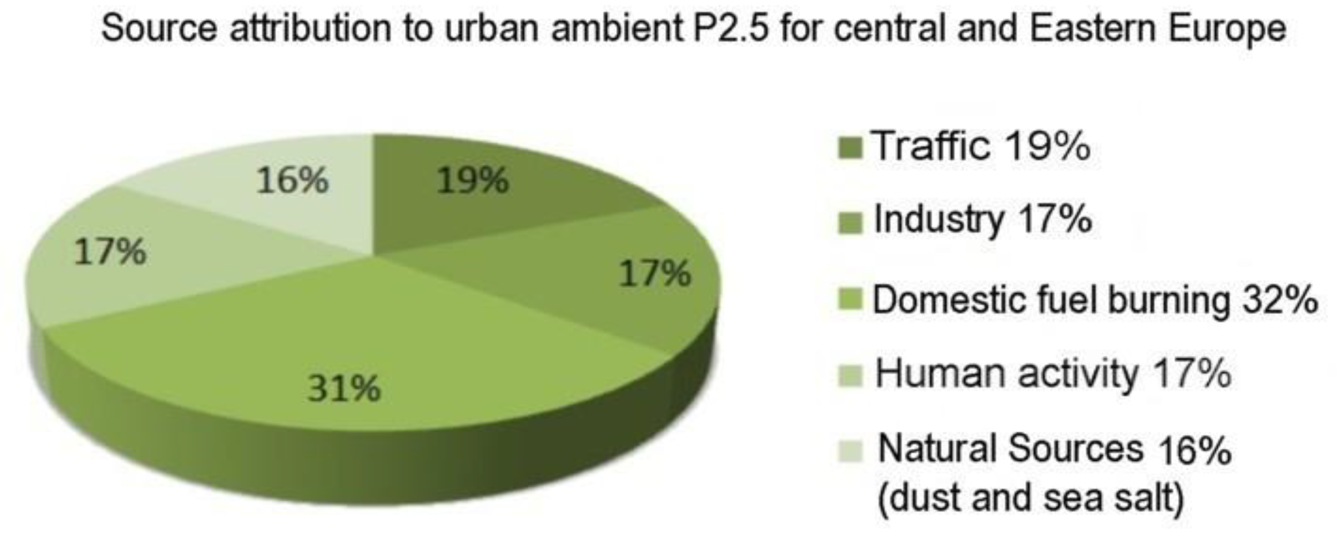
2.6. Sources of Air Pollution by Particulate Matter (PMF Numerical Methods of Outdoor Sources Apportionment)

The first databases on separate sources of air pollution (outside) of buildings with PM1 and PM2.5 dusts were created in2014 by the World Health Organization. These data were organised and collected by Karagulian et al. [46].
In order to reduce the health impacts of air pollution, it is important to understand the sources of pollutants contributing to environmental exposure. This study systematically reviewed and analysed the distribution of available sources for particulate matter surveys (10 and 2.5 microns in diameter, PM10 and PM2.5) performed in cities in order to estimate typical source contributions by country and region.
The percentage of separate sources of PM2.5 and PM10 dust in the urban environment for the Central and Eastern Europe region per source category according to the World Bank’s list of economies (2012) for Central and Eastern Europe, provided by [46], is shown in Figure 4.
The available records regarding the distribution of sources, however, show significant heterogeneity in the assessed source categories and incompleteness in some countries/regions.
In the years 2014–2017, receptor models tested using the PMF (Positive Factorised Matrices) method were increasingly used to isolate the sources of pollution in the outside air. The basis for the application of such a model by Samek et al. [36] in urban areas such as Kraków, where the levels of pollution often violate air quality standards, was the collection of measurement data on air pollution, especially PM2.5, considered to be the most hazardous to health. In 2014, approximately 200 samples were collected.
The lowest monthly concentration values were found for August 2014—around 10 μg/m−3.The highest was for February 2014—70 μg/m−3—while the annual average value was around 31 μg/m−3. Using the X-ray fluorescence method to test PM concentration, 15 elements were determined for each sample and eight inorganic ions were analysed by ion chromatography. Additionally, the samples were analysed for soot (PNE). The average concentration of PM2.5 in Kraków (31 μg/m−3) was twice as high as in 2009–2013 in Genoa, Barcelona and Florence, and similar to Milan.
A receptor model adapted to the research with the EPA PMF 5.0 program was developed, which was used to identify sources of air pollution with suspended dusts and chemical components (elements and ions) generated by separate sources. As a result of the modelling, six sources were identified. The sources of dust and their quantitative share in the total mass of PM2.5 was determined. The following sources have been identified: (1) Combustion, (2) secondary nitrates and sulphates, (3) biomass burning, (4) industry, (5) the soil and (6) road traffic. Monthly deviations of the efficiency of the source of pollution with PM2.5 dust are presented.
In the Warsaw area, the Juda-Rezler et al. [40] team also applied the positive matrix factorisation (PMF) method, supported by the analysis of enrichment factors, in order to identify the six main sources of PM2.5 dust: Residential combustion (fresh and old aerosols) (46% by weight of PM2.5), road fumes (21%) and unused exhausts (10%), mineral dust/construction works (12%), high temperature processes (8%) and steel processing (3%). In this analysis, primary organic carbon (POC) and secondary organic carbon (SOC) were classified as two separate components that helped distinguish between primary and secondary aerosol sources. Identification of the sources was also supported by the study of their annual and weekly profiles, as well as the analysis of the correlation of particulate components with meteorological conditions. Comparison of the attributed sources of air pollution with dust in Warsaw and Kraków is shown in Table 3.
The most expressive elements of PM sources in Warsaw are SOC, Cl and As for combustion in apartments, NH4+, Sb and POC for road transport, Ca and Mg for construction works, and SO42− for PM transport over long distances.
The analysis of the collected data, including carbon species, eight main water-soluble ions, 21 small trace elements and local meteorological conditions were used to assess the nature and seasonal variability of PM aerosols in Warsaw, as well as to identify the contribution of natural and anthropomorphic sources to the aerosol levels.
The method of studying the active sources of dust pollution from which the pollutants originate in school buildings located near Athens, Greece, was investigated by [47]. The tests using the PMF method were carried out in 2017 and they referred to the mass concentrations (the highest was 72.02 µg/m−3) and the chemical analysis of PM10. Seasonal fluctuations were also examined.
Lv et al. [10] studied the concentration of solid particles in Daqing China, from the outside Cout, and their percentages expressed in mass concentrations in buildings of various applications, as well as the correlations of internal pollution with the locations of buildings exposed to external sources of dust of various origins (office: Cout = 22 μg/m3 and ρ = 79.4% (ρ–contribution rate I/O of indoor and outdoor particle sources to the concentration of indoor particulate matter); classroom: 20 μg/m3 and 87.6%; city residence: 30 μg/m3 and 75.0%; rural house: 34 μg/m3 and 90.2%). The researchers found that the share of external sources in the concentration of PM indoors exceeds 70%, and in classrooms and in the countryside it exceeds 90%.

3. Materials and Methods

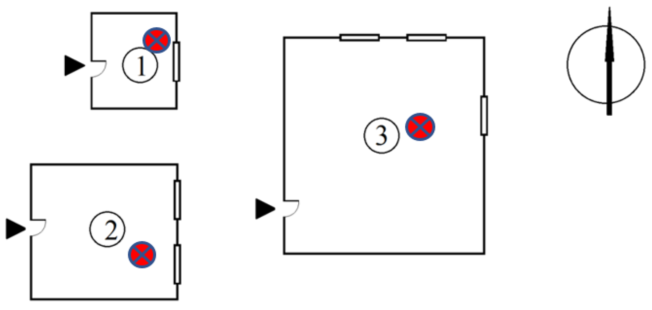
3.1. Preliminary Measurements of Mass Concentrations of Dust Pollutants Inside Rooms

There are two types of PM measurement instruments: Those that provide average concentrations over the sampling period and those that provide real-time instantaneous concentration monitoring. Instruments based on the gravimetric method are considered as reference methods and must meet the requirements of PN-EN 12341:2014 [48]. The principle of the reference method is to collect the particulates on a circular filter. This must be a glass fibre filter (GFF), a quartz fibre filter (QFF), polytetrafluoroethylene (PTFE) or PTFE-coated glass fibre, and must be thoroughly conditioned before and after collection. The filter itself should be weighed before and after collection.
Optical instruments based on light scattering, absorption or occultation of light by particles are used to measure dust concentration in real time. They must have certificates confirming their equivalence with the reference method.
A detailed description of the measurement strategy for airborne particles and legal measuring equipment can be found in ISO 16000-34:2018 [49] and ISO 16000-37:2019 [50]. Measurement of PM2.5 mass concentrations describes the strategies and procedures for measuring the mass concentration of PM2.5 indoors.
Tests of dust air pollutants in selected rooms were carried out from 27 January 2020 to 10 March 2020 in a low office building (two-story high), located in the centre of Warsaw in an urban development. Three office rooms with a different area and a different proportion of external and internal walls were selected for the study of air pollution. The rooms were empty, the leaks had been identified and taped over, leaving only airflow through the window vents and the undercutting of the front door. Localisation of the measurement devices in rooms is shown in Figure 5. The cubic volumes and number of windows of the analysed rooms were as follows:
  • Room 1–23.48 m3, 1 window
  • Room 2–48.75 m3, 2 windows
  • Room 3–93.14 m3, 3 windows
The rooms were situated on the ground floor of the building (approximately 2 m above ground level and 104 m above sea level). At the time of the test, the exhaust ventilation was turned off, and the ventilation was turned off one hour before the start of the measurements. In the immediate vicinity of the building in question, there are other office buildings and multi-occupancy residential buildings connected to the municipal central heating. In terms of height, the adjacent buildings can be characterised as low (height above ground level up to 12 m), medium (height above ground level up to 25 m) and tall (height above ground level up to 55 m). There are local access roads with low traffic around the office building in question. At a distance of approximately 120 m from the building in question, there is a main road with heavy traffic.

3.2. Measurement Methods (Measuring Instruments and Procedures of Particle Concentration Measurements Inside and Outside the Building)

Measurements of the mass concentration of dust inside were carried out by the AEROCET 831 Handheld Particle Counter (Met One Instruments Inc, Grants Pass, OR, USA) operating on the optical principle with a laser diode, and by the TSI QUEST EVM-7 optical-gravimetric environment monitor, indicating the mass concentration of particles, but also their size fractions PM2.5, PM4, PM10 (in terms of measuring the particle size distribution, the optical device is classified as a laser light scattering aerosol spectrometer—LSAS—for measuring particle sizing). The TSI QUEST EVM-7 environment monitor (TSI INCORPORATED, Shoreview, MN, USA) also measures the CO2 concentration inside the rooms. Used equipment is shown in Figure 6. Used devices are under the supervision of the environmental laboratory and are regularly checked and periodically calibrated. Each device was checked and calibrated before the experiments. Meters from Table 4, the dust and environmental condition measuring devices AEROCET and the TSI were set to zero prior to the measurement using the “filter 0” in order to “reset” the measurement path.
The operating principle of a LSAS relies on particles being guided individually through an intensely illuminated volume. Commercially available equipment enables the particle mass concentrations to be estimated and displayed by the monitor, using evaluation software. Normally, these programs assume the ideal spherical form of particles and convert them to mass concentration. Calibration of the TSI QUEST EVM-7m is required and usually performed with PM latex particles of a defined diameter as the test aerosol. A comparison with other gauges should, however, always be made carefully because ultimately what is determined by LSAS is the particle equivalent optical diameter determined by calibration with monodisperse spherical latex particles.
The lower detection limit depends very much on particle size: The larger the particles, the lower the limit of quantification. The characteristics of the devices used for measuring the internal environment, including PM10 and PM2.5 dust, are shown in Table 4 below.
Outdoor concentrations of PM10 and PM2.5 on both measurement days will be based on CIEP-Chief Inspectorate of Environmental Protection, pol. GIOŚ archival data and the results of measurements made with the AEROCET 831 m.
At CIEP, dust concentrations were measured using an automatic method, by a CIEP environmental monitoring station located closest to the building selected for the study. CIEP provides access to hourly monitoring data on air quality in Poland, produced as part of the State Environmental Monitoring and collected in the JPOAT2.0 database.
The CIEP pollution measurement stations taken into account during the tests differ from each other in terms of their location, as well as their location in relation to communication routes affecting the measured pollution levels.
At the same time, measurements of the mass concentration of PM10 and PM2.5 were performed using the AEROCET 831 m described in Table 4, placed outside, right next to the window opening of the monitored room, i.e., outside the building. Due to the use of different devices at the Building Research Institute and CIEP, the not fully established measurement procedure of “outside the window” (a critical increase in the AEROCET 831m indications was noticed when the cleaner was turned on), different distances and positioning of the monitored rooms in relation to the sides of the world from the official air quality control points, the results of the present study’s measurements are not fully comparable with the results presented by CIEP. Self-readings of outdoor concentrations should be more reliable for comparison because they were carried out at the same time points as the indoor pollutant concentration. The outdoor environmental parameters were observed and recorded during experimental campaign. In these preliminary tests, the air velocity in the immediate external environment was not measured.
During the measurements of the mass concentration of dusts, the concentration of CO2 was also measured with the TSI QUEST EVM-7 m in each test room.
The measurements of the time curves of decay (measuring particle decay curve) and the particle concentration rebound curve in the interiors were carried out in time cycles of 150 min. The concentration of suspended dusts was rebuilt as a result of natural dust penetration through the external wall of the building and the gaps near windows and doors in the time period of from −50 to 0 min, as the cleaner was turned on in the time interval from 0 to 150. At point 0 (on the x-axis), when the cleaner was switched off, the indoor dust concentration was measured and had a minimum value. The second part of the transient curve is the concentration rebound curve.

3.3. Procedures for Measurements of PM2.5 Mass Concentration in the Indoor Mode Performed at ITB

During the tests, which were carried inside each room on three days, when the air pollution by PM2.5 outside was different, the following weather conditions were recorded, as shown in Table 5.
Indoor air pollution tests in three selected rooms were carried out according to the following scheme:
  • An initial measurement of the concentration of PM10, PM2.5 and CO2 was performed.
  • The Samsung AX90R7080WD/EU air cleaner was turned on and PM mass concentration measurements were performed until the minimum dust concentration was achieved.
  • After turning off the air cleaner, measurements of the concentration of PM10 and PM2.5 dust were taken until reaching “saturation”—the state where indoor PM concentration no longer decreases.
  • After achieving the point of a steady state of PM concentration the measurements of the concentration of PM10 and PM2.5 dust were going on until reaching equilibrium of I/O concentration.
Thus, this study measured the transient concentration decay curves of the decrease in dust concentration in the room after the air cleaner was turned on until it was turned off at point Cin,0, and the transient PM concentration rebound curves of the recovery of dust concentration in specific time intervals determined on a real-time basis. The particle concentration rebound curves not the particle concentration decay curves were used in our research to measure the penetration factor. This modification of the method is to be used for determining the value of the particle deposition rate k not from the course of the characteristics in the transient state, the so-called particle decay curve, but from the course of the further time stimulated by infiltration, the so-called particle concentration rebound curve. This method was used to determine the value of k and then P was recognized as correct by He [25] andDiapuoli [51] but it has not been used so far.
One person stayed in the room during the measurements, hence the constant increase in the concentration of carbon dioxide, which was also measured with the TSI QUEST EVM-7 m.
The CO2 concentrations marked as c0 and ct were measured on each measurement day at the beginning and at the end of the measurements of PM2.5 mass concentrations.
The results of CO2 concentration measurements in room 1 (with one window) and in room 3 (with three windows) in ppm are given in Table 6 (assumed CO2 concentration outside equal to 500 ppm); according to the statement of the Minnesota Department of Health: ‘The outdoor concentration of carbon dioxide is about 400 parts per million (ppm) or higher in areas with high traffic or industrial activity. The present authors’ assumption is determined by localisation of the measurements points and their own experience in this area.
Dust concentration tests in individual rooms were carried out sequentially (not simultaneously); therefore, the external environment for rooms 1–3 may differ slightly.

4. Results and Discussion

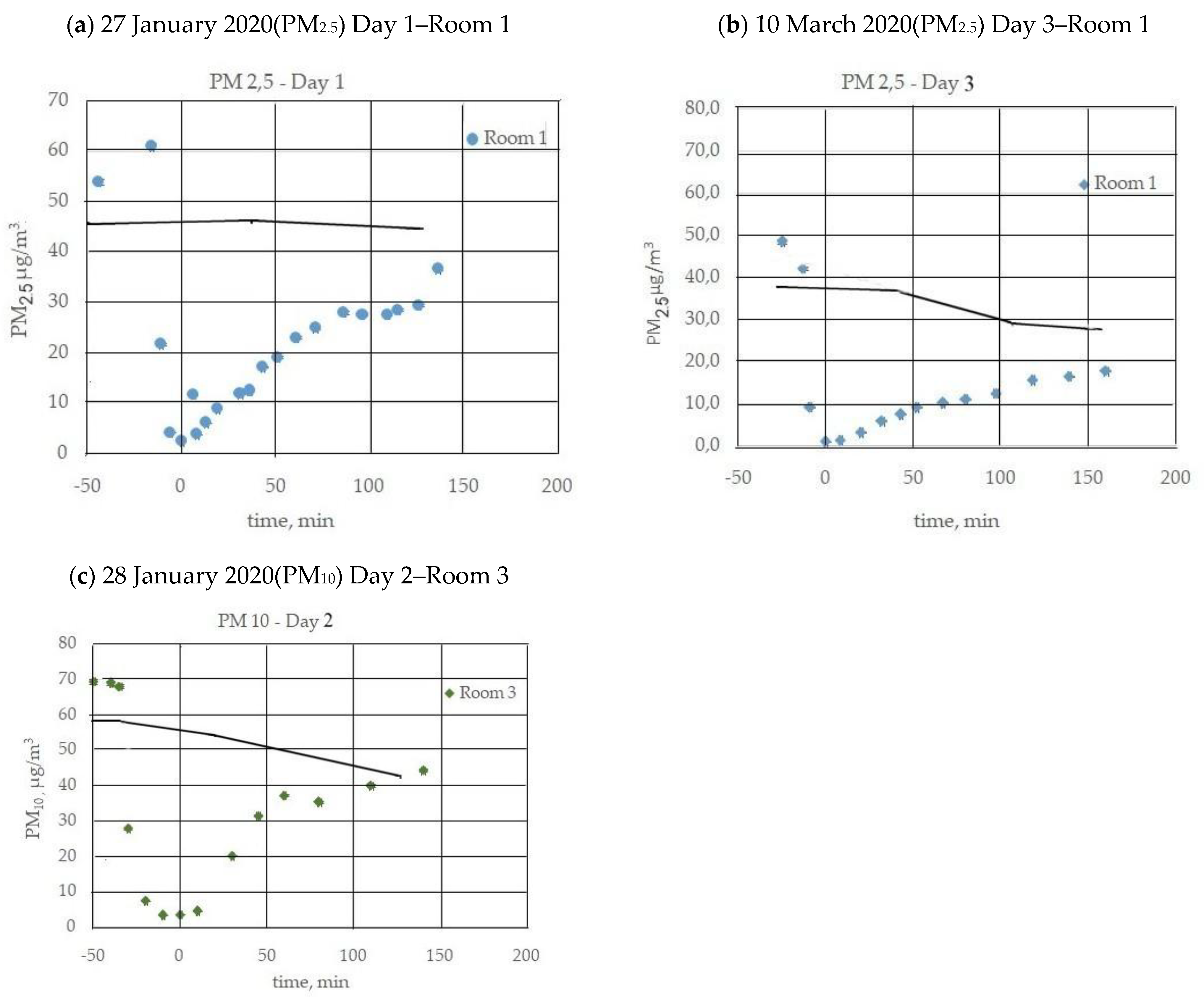
4.1. Results and Discussion of Preliminary Measurements of Indoor PM2.5 and PM10 Concentrations

The concentrations of PM10 and PM2.5 outside were taken from published data on the basis of measurements made by the CIEP Environmental Protection Station closest to the studied rooms (Warsaw, Wokalna 7and Al. Niepodległości 227/233). Measurements of air quality stations are reported with an hourly interval and shown in Table 7.
Based on the data on dust concentrations obtained from the hourly monitoring of the Chief Inspectorate of Environmental Protection for PM10 and PM2.5 dusts on Day 1 (27/01/2020), Day 2 (28/01/2020) and Day 3 (10/03/2020), the curves of dust concentration changes outside the building were determined. The curves of dust concentration inside the building in the indicated rooms were drawn on the basis of measurement data made with the AEROCET 831 m. Figure 7a–c show changes in the mass concentration of PM10 and PM2.5 on the first, second and third days of measurements in rooms 1 and 3.
Comparing the measurements of PM2.5 dust on day 1 (Figure 7a) and day 3 (Figure 7b) in room 1, it can be concluded that the rate of dust concentration level increase was higher on day 1, and the indoor pollution equilibrium state was reached by approximately100 min. The rate of dust concentration level was much lower on day 3, and the indoor pollution equilibrium state was reached by approximately150 min. This may be due to the smaller and continually decreased PM concentration gradient (Cout–Cin) (although at the same time during the measuring cycle, the temperature and wind speed were slightly higher). On day 3, the ambient concentration of dusts Cout measured by CIEP decreased in measuring time from 38 to 28 µg/m3.
By analysing the course of the measurement of PM10 on day 2 (Figure 7c) in room 3, it is possible to notice also a uniform decrease in pollution outdoors caused by high relative air humidity; therefore, the concentration gradient (Cout–Cin) also decreased. According to theoretical assumptions, however, the equilibrium level of PM10 concentration inside the room is set at a level about 40% higher than the level of PM2.5 concentration (Figure 7a). The measurement of the PM10 concentration rebound curve (Figure 7c) was completed when rainfall occurred. Authors found that the compliance between the CIEP (Chief Inspectorate of Environmental Protection) results with our PM2.5 measurements outside the building is of the order of uncertainty in the measurement of PM concentrations inside regarding the used field instruments in accordance with Table 4.
Obtained results of preliminary experiments have shown that a system for measuring the concentration of PM2.5 directly outside the window should be designed, which would be protected against disturbances caused by the operation of the air cleaner in the interior and changes by the meteorological parameters.

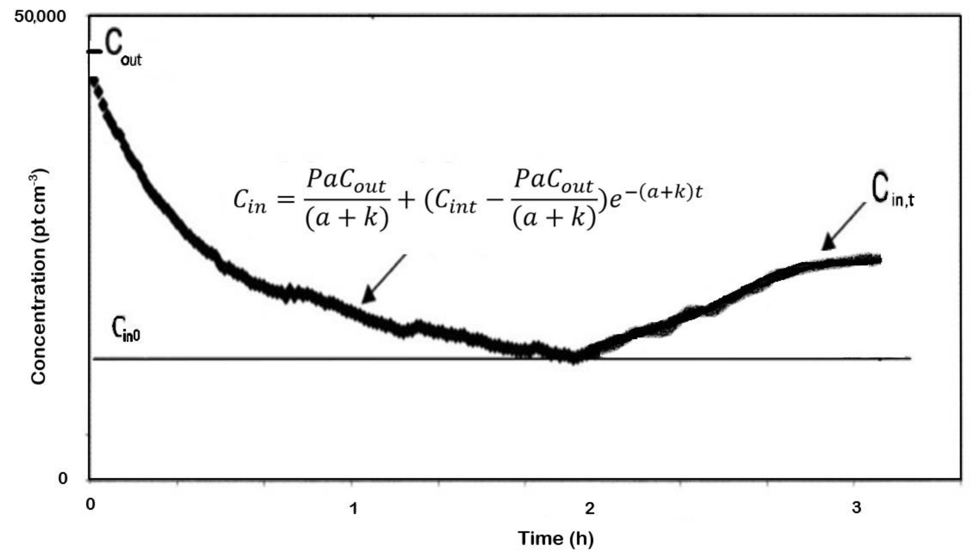
4.2. Theoretical Basis and Possibilities of Predicting Dust Penetration through the Building Envelope. A Dynamic Model of the Mass Balance Equation of Indoor Particle Concentration Levels

The process of penetration of dust from the outside into the interior of the building and the generation of PM by internal sources is a dynamic process [46]; therefore, all findings emphasise the importance but also the difficulty of determining separately the time courses of changes in the concentration of suspended dust in the interior, and the share in their mass of suspended particles from outdoors and the proportion of particles generated indoors. Such data are necessary for the interpretation of the results of epidemiological studies. In this framework, recent scientific research has focused on the study of factors influencing the penetration of particles through the building envelope and the quantification of the relative indoor proportion of particles coming from outside and remaining as dust suspended inside the room. The basic form of the dynamic mass balance equation is given in [25,51,52,53,54,55,56]; it describes the profiles of changes in the temporal concentration of PM during the particle decay curve or during the reconstruction of this concentration (particle rebound curve) in the room with Equation (4)
d C i n ( t ) d t = a · P · C o u t ( t ) ( a + k ) · C i n ( t ) + Q i s V
where Cin(t) and Cout(t) are the concentrations of particles inside and outside at time t, respectively (mg/m3); a is the multiplicity of air changes (h−1); P is the dimensionless coefficient of particle penetration efficiency; k is the particle deposition rate (h−1); V is the volume of the interior (m3); and Qis is the rate of generation of particles by the indoor sources(mg/h). Equation (4) assumes perfect mixing of indoor air. It also ignores particle mass losses or gains due to differences in the gas-phase concentrations of condensable substances and changes in temperature/relative humidity conditions between indoor and outdoor spaces. The penetration efficiency factor (P) and particle deposition loss rate (k) are also related to building characteristics and indoor/outdoor conditions, but these parameters also depend on particle size, composition and their electric charge.
The particle penetration factor (P) is defined as the mass fraction of the particles in the infiltrated air passing through the building envelope, which depends on particle diameter (dp). This simple definition is
P = N e s c a p e / N t o t a l
where Nescape are the particles escaping through the leak outlet and Ntotal are the particles collected at the entrance of the leak in the building. The penetration factor is the most appropriate parameter for describing the mechanism of particle penetration through cracks and leaks in the building envelope, and at the same time the parameter describing the functionality of the building and, thus, its balance.
The main difficulty in the solution to this equation lies in the separate calculation of the penetration efficiency factor (P) and deposition rate (k). The values for these two parameters that are reported in the literature vary significantly. Deposition rate k presents the widest range of values in terms of size fractions in the literature. The penetration efficiency factor P seems to be more accurately calculated through the application of dynamic models.
Bennett and Koutrakis [57] developed a method for calculating the unknowns (P) and (k) using time-dependent indoor and outdoor particle concentrations and air exchange rate (a). Assuming there are no indoor particle sources, when using discreet time steps Δt, expressed as Equation (4), Equation (6) can be rewritten as follows
C i n , t = a i P i C o u t , t Δ t ( k + a i ) × ( 1 e ( k i + a i ) Δ t ) + C i n , t Δ t × e ( k i + a i ) Δ t
Assuming steady-state conditions inside the building, no internal sources of suspended dust generation and no mechanical ventilation with a filter, Equation (6) can be transformed into a Equation defining the dust infiltration coefficient Finf. The infiltration of air with particles suspended indoors is also described by the infiltration coefficient (Finf), which determines the fraction of external particles that enters the internal microenvironment and remains suspended. The particulate matter infiltration process is defined by the following equation
F i n f = C i n C o u t = P · a a + k
where Finf is the PM infiltration factor (-).
“When indoor particle emissions cannot be avoided, the method developed by Long et al. [58] which is based on the linear regression approach can be used for Finf determination”.
The analytical solution of Equation (6), based on field measurements of mass concentrations of PM2.5 inside and outside the building was used by Chao Chen et al. [59] in their study of particle penetration through window gaps. They used Equation (6), where the Δt is time step Δt = 1 h; and ai, Pi, ki are hourly air exchange rate, penetration factor and deposition rate, respectively. Therefore, Equation (6) can be resolved when Cin,t and Cout,(i = 1, 2 … n) are known for a period Δt of time, where hourly indoor and outdoor PM2.5 mass concentrations could be determined by field measured data, so the unknowns are air exchange rate (ai), penetration factor (Pi) and deposition rate (ki). As such, the number of equations is (n − 1) and the unknowns are 3(n−1) in the new Equation (4) (n − 1, ai, Pi and ki).
The experimental solution of the dynamic mass balance equation of indoor PM concentration is recommended by [25,52,53]. They argued that a dynamic variation of the PM concentration level in the sample room should be performed while simultaneously measuring the PM particle decay curve in real buildings.
When the test time is longer than the time constant, it is implied that the indoor PM2.5 concentration has reached a steady-state condition, then
d C i ( t ) d t = 0
Therefore Equation (4) can be summarized by Equation (9)
C i n , t = C i n ( 0 ) = P · a · C o u t a + k
where Cin,t is the steady-state indoor PM2.5 concentration.
Upon determining the “decay term” (a + k) and the air exchange rate a, the penetration efficiency factor P is described by the following equation, which assumes the absence of internal sources PM.
P = ( a + k ) a · C i n , 0 C o u t
where C i n , 0 is the concentration Cin of the PM particles already at a steady state with time.
By estimating the coefficient of particle infiltration from outside into the room, Finf, from the dynamic mass balance equation, it is difficult to determine independently the values of P and k. Over the last two decades, many methods have been used to estimate P and k and calculate the relative contributions of particles from indoor and outdoor sources in the measured mass concentrations of given indoor particles. Diapouoli et al. [51] describe a broad overview of the methods for determining the values of these parameters, presenting different approaches, which they grouped into four categories according to the principles of their determination: (1) Steady-state assumption using the steady state of the mass balance equation; (2) dynamic solution of the mass balance equation using complex statistical techniques; (3) experimental studies using conditions that simplify model calculations (e.g., decreasing the number of unknowns); and (4) infiltration surrogates using a particulate matter (PM) constituent with no indoor sources to act as surrogate of indoor PM of outdoor origin. As they claim, however, the analysis of various methodologies and results shows that the estimation of particle infiltration parameters is still difficult.
The penetration factor P measurement principle, according to the authors’ proposal, covers the realisation of the dynamic mass balance equation of indoor PM concentration, which is presented in Figure 8. Air exchange rate a is measured at first using the properly documented principle and therefore it is not described in Figure 8.

4.3. Method of Determination of the Penetration Efficiency Factor P

Air exchange rate in the internal microenvironment (a)
The rate of air exchange in the room (a) due to infiltration of air from the outside is a measurable parameter, and is mainly influenced by the construction and technical condition of the external wall of the building and the ventilation system, the activity of residents and meteorological conditions.
The size of (a) in the room where people are present can be estimated on the basis of the time curve of the decay of CO2 concentration in the room at night. The air exchange rate can be estimated from the exponential curve of decay of CO2 concentration over time, using Equation
a = 1 t t 0 ln ( c c o u t c 0 c o u t )
where a is the air change rate (h−1), and the values of time t and t0 are read at the end and the beginning of the concentration decay curve (h−1), respectively. The values of c and c0 are CO2 concentrations (ppm) measured at times t and t0, respectively, and cout (ppm) is the concentration of PM outside at time t. The air change rate estimated for different measurement cycles shows seasonal fluctuations in the multiplicity of air changes. In naturally ventilated buildings, air flow is caused by differences in temperature or pressure inside and outside the building.
Equation (11) was used by the Czech–Norwegian team of Chatoutsidou et al. [54] in a study of the infiltration process in The Baroque Library Hall building in Prague with a natural ventilation system by infiltration in order to calculate the number of air changes. In this study, a dynamic mass balance model was used, taking into account the penetration of particles from external and internal losses (deposition, ventilation). The model was used to determine the particle deposition rate k and the penetration efficiency P. As a result of the three-year research, the values of a for spring were a = 0.13, for summer a = 0.11 and for winter a = 0.15. Equation (11) was also used in a simplified form by [25,60].
a = 1 t ln c t c 0
Deposition rate of airborne particles (k).
One of the simpler methods of determining the particle deposition coefficient is recommended by [25,51], who specified the factor of Equation (6) as the “decay term”—(a + k) in the time interval Δt, using the regression analysis of the experimentally determined particle concentration decay curve. The temporary disappearance of the dust concentration in the interior, i.e., the Cin0 concentration, to the Cint highest concentration (e.g., Cin level caused, for example, by the operation of the air cleaner) in accordance with equation
ln ( C i n , 0 C i n t ) = ( a + k ) Δ t
is used to then derive the value of k from the value (a + k). An increasing trend was found for increasing particle sizes. At the maximum particle size, particle deposition rates are of the same order or even higher than their removal rates due to blown air exchange. According to the results of [1], higher deposition rates were found for larger particles, so the deposition coefficient k of PM10 particles is greater than k for PM2.5 particles. They also found large differences in deposition rates among the six residences studied as a result of a discrepancy in surface material texture and roughness as confirmed by Abadie et al. [61]. They also demonstrated that the deposition effect is temperature dependent.
Particle penetration efficiency through the external walls of the building (P).
There are several different models in the literature for predicting the penetration efficiency P of particles through the gaps in the building envelope. The equation resulting from the Lagrangian model (Chen, Zhao [52]) is particularly interesting. It calculates the trajectory of each particle by integrating the equilibrium forces acting on individual particles.
The practical significance of the research conducted by Chao et al. [62] from the Hong Kong Technical University concerned the determination of the P and k coefficients in residences with natural ventilation. Both parameters were dependent on particle size but showed a different upward and downward inversion profile with respect to particle size. The main causes of loss by deposition and penetration effects are diffusion, inertial impact/interception and deposition (showing a different up-and-down inversion profile against particle size).
The efficiency of P is related to particle size, as demonstrated by many researchers who compared the penetration of particles of different sizes [1,25].
Chao et al. [62] studied six buildings and argued that ‘the penetration coefficient showed a hill-shape with respect to particle sizes and there was a peak (0.79) at the size range of 0.853–1.382 µm’.
It follows that the deposition coefficient k of PM10 particles is greater than k of PM2.5 particles while the penetration coefficient P of PM10 particles is less than P of PM2.5 particles. The P particle penetration factor is, therefore, another important factor determining the value of the I/O ratio. If the building is ventilated by infiltration, however, the expansion of the particle penetration coefficient is a strong function of the air exchange coefficient a, particle size and fracture geometry in the building envelope.
Chao et al. [62] also described a simplified way to analyse the model of indoor particle behaviour.
This simplified method has been developed for users of particle counters, who need to express concentrations in the form of a particle number concentration, i.e., (×103) p cm−3, so that there is a need to convert the units in which the particle concentrations are recorded, i.e., convert the particle mass concentration units µg/m−3 per unit of particle number concentration (×103) p cm−3, assuming a spherical shape and uniform particle density and packing. Such conversions are performed for each particle size range.
Returning to the dynamic mass balance Equation (6), it can be said that all parameters in this equation are known values, except for the penetration efficiency coefficient P and the deposition rate k. Chao et al. [62] transformed Equation (6) into a transient form. For each particle size range, the concentration of particles in the interior during the forced change in dust indoor concentration is equal to Equation (14)
C i n = P a C o u t ( a + k ) + ( C i n t P a C o u t a + k ) e ( a + k ) t
where Cint the is the initial dust pollution on the transient concentration decay curve.
Equation (14) consists of two parts: P·a·Cout/(a + k) and (a + k), which are the steady-state particle concentration and the time constant of the transient term, respectively.
Chao et al. [62] performed an experiment of the process of particle concentration decay of Cin at time (t–to) caused by intensive cleaning of the room from particles using an air cleaner. A typical profile curve of such a process is given by [62] and is also cited by [63]. The experiment consisted in artificially increasing the PM concentration to the Cint highest concentration value in the room in order to obtain a “drive” for the increase in the deposition rate, and then quickly reducing the concentration of solid particles to the steady state Cin0 by inducing ventilation present in the building. Substituting all measured particle concentrations and the air exchange rate a obtained in the tracer gas CO2 decay test, the deposition rate from the particle decay curve can be expressed as follows:
k = ( 1 t ) ln ( C i n C i n 0 C i n t C i n 0 ) a
The difficulty in applying this equation, however, lies in the correct choice of the time point in particle concentration decay curve at which the k value is to be calculated, since the chosen value of t will determine the value of Cin(t) from the decay curve or from the particle rebound curve. The penetration rate P can be found from the steady-state particle concentration upon determining the deposition rate k, which is shown as follows:
P = ( 1 + k a ) C i n 0 C o u t
The penetration factor consists of the ratio of the concentration found inside to the level of particle concentration outside (I/O ratio) and from the expression to the ratio of the particle deposition rate to the air exchange rate. In the case where the deposition rate k is much slower than the air exchange rate a, the penetration coefficient is equivalent to the I/O ratio.
The particle decay method can be replaced by the particle concentration rebound method as mentioned by [25,51,52]. Then, it will be a reversed process, the transition curve of which will reflect more closely the ease of particle penetration. This is because the experiment takes place under conditions of natural pressure difference I/O, and reflects better the efficiency of penetration of particles through the building envelope.

4.4. Exemplary Determination of the Penetration Efficiency Factor Based on the Results of Tests of the Profile of Forced Changes in the Concentration of PM Particles in a Selected Room

As an example of a measurement cycle, the results of which were used to calculate the value of the penetration efficiency factor P of PM2.5 particles through the external walls of the building, we chose the mass concentration Cin and Cout measurement cycle of 27 January 2020, made in room 1 (with one window), and presented in Figure 7a.
Assuming that for further calculations of the penetration coefficient, an experiment must be conducted that will force the concentration decay process, and then the process of restoring the concentration level of PM2.5 in the selected room (as in experiments in [26,62]), the authors present the transient curve of this dynamic process with the penetration of PM2.5 particles through the building envelope in Figure 7.
The first step was to determine the value of the air changes rate a in the selected room and under the thermal conditions of the measurement cycle. The CO2 concentrations marked as c0 and ct were measured on each measurement day at the beginning and at the end of the measurements of PM2.5 mass concentrations. The values of CO2 concentration outside the building, cout = 500 ppm, were assumed in accordance with ISO 16000-26:2012 [64]. The a value calculated from Equation (9) was for the selected room and measurement date a = 0.28.
The value a (ACH air changing rate h−1) is calculated from equation
a = 1 ( t t 0 ) ln ( c t c o u t ( c 0 c o u t ) )
In order to use Equations (14)–(16), the authors had to convert the results of particle concentration measurements in the selected measurement cycle (Figure 9) from the mass concentration units μg/m−3 to the numerical concentration units (×103) p/cm−3 (number of particles to cubic cm). The method of conversion was taken from the article by Morawska et al. [26], assuming (for the size range of PM2.5 particles) the conversion factor of 21.3/18 of the values of mass concentration units to units of numerical concentration.
The second step is to determine the value of particle deposition rate k (from the concentration decay curve Cin of PM2.5 particles or from the particle concentration rebound curve (see Figure 7) in the selected time interval Δt (then, it is a reverse cycle) in the room under the conditions of the determined air change rate a (see Table 8). The k factor will be calculated for the measurement cycle shown in Figure 7, using Equation (7) simplified to the form (13) with the data from Table 9.
From the PM2.5 particle concentration decay curve measured in Room 1 on 27 January 2020 (Figure 8) curve segment Δt = t-t0 of the particle concentration rebound curve was selected. Cin0 = 4.5 × 10³ p cm−3 was calculated for time t0 and Cin = 30.7 × 10³ p cm−3 was calculated after 60 min for break point t of the particle level restoration curve. Based on Equation (13), the value (a + k) = 1.90 was determined, which gives, after subtraction, a = 0.28 and k = 1.62
Calculation of the value of k (deposition rate h−1) from Equation (13)
ln ( C i n 0 C i n , t ) = ( a + k ) Δ t
In the literature, however, there is a large discrepancy in the values of the deposition rate factors for the size range of PM2.5 particles, which are reported with the values of the air exchange rate.
In the range of a from 0.45 to 0.61 h−1, i.e., in conditions similar to our air changing rate a = 0.28 h−1, the value of k = 2.01 ± 1.11 h−1was given in He, Morawska and Gilbert [25].The authors decided to compare the obtained value with others, e.g., Chao et al. [62] (k = 0.53 h−1 to k = 1 h−1). We chose our value of k = 1.62 h−1 for further calculations because it is close to that given by [25] and because previously a similar value of k = 1.3 h−1 for PM2.5 was obtained by the team Thatcher et al. [65] from the Lawrence Berkeley National Laboratory.
The third step is to calculate penetration P from Equation (16) with the data from Table 10.
P = ( 1 + k a ) C i n 0 C o u t
Thus, after converting the values of Cin0 = 4.5 × 10³ p/cm−3 and Cout = 52.0 ×10³ p/cm−3, and substituting all parameter values into Equation (16), the value P = 0.61 is obtained. From the course of the measurement cycle (Figure 7a), it can be seen that the value of P will be higher because the concentration level of Cout during the particle concentration rebound curve measurement was constantly decreasing.
The value is verified by the data collected by Chao et al. [62] who, based on their research, compiled the values of P factors for particles in wide particle size ranges.
For PM2.5, it is possible to determine the P value of PM2.5 particles by interpolating the P factor value from the chart prepared by Chao et al. [62]. The calculated value P = (2.458 + 2.642)/2 = 0.63 is roughly consistent with our value P = 0.61.
According to a recent study by Yu et al. [38], in diverse pressure differences, the 0.25–2.5 µm particles within the scope of penetration factor P is close to 1, which increased along with the pressure difference between the two sides of the gap. Four penetration factor models compared Chen and Zhao [52] and present much lower P values for PM2.5.

5. Conclusions

Predicted infiltration factors Finf in urban residences were collected, tested and classified by Baxter et al. [66] from the Harvard School of Public Health in Boston. They studied various factors related to occupant behaviours and home characteristics, which might influence ventilation patterns or infiltration factors. These include age of construction, housing type (multi- vs. single-occupancy homes), floor levels, opening windows, seasonal differences in Finf and air conditioning or HVAC system use.
The transport of outdoor particles across the building envelope (i.e., penetration) is an important physical factor that contributes to particle concentration and size distribution inside buildings. The penetration factor can be equalised when doors and windows are open, but under different conditions the p values ought to be measured.
Outdoor pollution sources, rather than indoor pollution sources, are the principal contributors causing indoor particulate pollution in modern office buildings. When there are no substantial indoor particle pollution sources, 60–70% of the indoor PM2.5 mass density comes from outdoor particulate pollution, according to the study.
This paper presents a modified method of determining the parameters of the process of penetration of PM2.5 particles through leaks in the external walls of the building with the use of the processes of natural recovery of the levels of particle concentration. So far, dynamic tests of PM infiltration have been performed using the blower-door depressurization procedure by introducing the n-th power disturbance in the air flow caused by increasing the pressure gradient in the I/O system. The modified method promotes the measurement of Cin concentration during the process of equalizing the level of PM2.5 concentrations inside and outside the building.
The preliminary results of the penetration factors determined by this method are consistent with the P factor values from the literature obtained so far for this dimensional group of dusts. Information on the P factor value can be a reliable parameter that classifies buildings in terms of resistance to dust infiltration into their interior, which may have a significant impact on indoor air quality. Obtained results of preliminary experiments have led to the conclusion that a system for measuring the concentration of PM2.5 directly outside the window should be designed, which would be protected against disturbances caused by the operation of the air cleaner in the interior and changes by the meteorological parameters.
The authors have tried to describe the current state of knowledge in the field of research on interior pollution by dust and establish a roadmap for launching and improving measurement and test methods so that in the future a dynamic indoor particle model could describe indoor air quality, when exposure to PM2.5 takes place. This model will be further tested using the Monte Carlo method before being included in the Combined IAQ model (Piasecki, Kostyrko [67,68]).

Author Contributions

Conceptualization, K.B.K. and D.B.; methodology, K.B.K. and D.B.; validation, K.B.K. and D.B.; formal analysis, K.B.K. and D.B.; investigation, K.B.K. and D.B.; resources, K.B.K. and D.B.; data curation, K.B.K. and D.B.; writing—original draft preparation, K.B.K. and D.B.; writing—review and editing, K.B.K. and D.B.; visualization, K.B.K. and D.B.; supervision, K.B.K. and D.B.; project administration, K.B.K. and D.B.; funding acquisition, K.B.K. and D.B. Both authors have read and agreed to the published version of the manuscript.

Funding

This research received no external funding.

Institutional Review Board Statement

Not applicable.

Informed Consent Statement

Not applicable.

Data Availability Statement

Data supporting reported results can be found in the Thermal Physics, Acoustics and Environmental Protection Department, Instytut Techniki Budowlanej, Warsaw, Poland.

Conflicts of Interest

The authors declare no conflict of interest.

References

  1. Thatcher, T.L.; Layton, D.W. Deposition, resuspension, and penetration of particles within a residence. Atmos. Environ. 1995, 29, 1487–1497. [Google Scholar] [CrossRef]
  2. Arvanitis, A.; Kotzias, D.; Kephalopoulos, S.; Carrer, P.; Cavallo, D.; Cesaroni, G.; Brouwere, K.D.; de Oliveira-Fernandes, E.; Forastiere, F.; Fossati, S. The index-pm project: Health risks from exposure to indoor particulate matter. Fresenius Environ. Bull. 2010, 19, 2458–2471. [Google Scholar]
  3. Crouse, D.L.; Peters, P.A.; Hystad, P.; Brook, J.R.; van Donkelaar, A.; Martin, R.V.; Villeneuve, P.J.; Jerrett, M.; Goldberg, M.S.; Pope, C.A., III; et al. Ambient PM2.5, O3, and NO2 exposures and associations with mortality over 16 years of follow-up in the canadian census health and environment cohort (CanCHEC). Environ. Health Perspect. 2015, 123, 1180–1186. [Google Scholar] [CrossRef] [Green Version]
  4. Hvelplund, M.H.; Liu, L.; Frandsen, K.M.; Qian, H.; Nielsen, P.V.; Dai, Y.; Wen, L.; Zhang, Y. Numerical investigation of the lower airway exposure to indoor particulate contaminants. Indoor Built Environ. 2019, 29, 575–586. [Google Scholar] [CrossRef]
  5. Wang, S.; Inthavong, K.; Wen, J.; Tu, J.; Xue, C. Comparison of micron- and nanoparticle deposition patterns in a realistic human nasal cavity. Respir. Physiol. Neurobiol. 2009, 166, 142–151. [Google Scholar] [CrossRef] [PubMed]
  6. Lin, Y.; Zou, J.; Yang, W.; Li, C.-Q. A Review of Recent Advances in Research on PM2.5 in China. Int. J. Environ. Res. Public Health 2018, 15, 438. [Google Scholar] [CrossRef] [PubMed] [Green Version]
  7. Lee, J.Y.; Ryu, S.H.; Lee, G.; Bae, G.-N. Indoor-to-outdoor particle concentration ratio model for human exposure analysis. Atmos. Environ. 2016, 127, 100–106. [Google Scholar] [CrossRef]
  8. Branco, P.; Alvim-Ferraz, M.D.C.; Martins, F.; Sousa, S. Children’s exposure to indoor air in urban nurseries-part I: CO2 and comfort assessment. Environ. Res. 2015, 140, 1–9. [Google Scholar] [CrossRef] [PubMed] [Green Version]
  9. Kalimeri, K.K.; Bartzis, J.G.; Sakellaris, I.A.; Fernandes, E.D.O. Investigation of the PM2.5, NO2 and O3 I/O ratios for office and school microenvironments. Environ. Res. 2019, 179, 108791. [Google Scholar] [CrossRef]
  10. Lv, Y.; Wang, H.; Wei, S.; Zhang, L.; Zhao, Q. The Correlation between Indoor and Outdoor Particulate Matter of Different Building Types in Daqing, China. Proc. Eng. 2017, 205, 360–367. [Google Scholar] [CrossRef]
  11. Nadali, A.; Arfaeinia, H.; Asadgol, Z.; Fahiminia, M. Indoor and outdoor concentration of PM10, PM2.5 and PM1 in residential building and evaluation of negative air ions (NAIs) in indoor PM removal. Environ. Pollut. Bioavailab. 2020, 32, 47–55. [Google Scholar] [CrossRef] [Green Version]
  12. Bai, L.; He, Z.; Li, C.; Chen, Z. Investigation of yearly indoor/outdoor PM2.5 levels in the perspectives of health impacts and air pollution control: Case study in Changchun, in the northeast of China. Sustain. Cities Soc. 2019, 53, 101871. [Google Scholar] [CrossRef]
  13. Zhang, S.; Duan, Y. Determination the PM2.5 concentration in the room of Liting mosquito-repellent incense and cigarette. Inn. Mong. Environ. Sci. 2013, 25, 184–185. [Google Scholar]
  14. Zhang, N.; Han, B.; He, F.; Xu, J.; Zhao, R.; Zhang, Y.; Bai, Z. Chemical characteristic of PM2.5 emission and inhalational carcinogenic risk of domestic Chinese cooking. Environ. Pollut. 2017, 227, 24–30. [Google Scholar] [CrossRef] [PubMed]
  15. Xue, Y.; Zhou, Z.; Nie, T.; Wang, K.; Nie, L.; Pan, T.; Wu, X.; Tian, H.; Zhong, L.; Li, J.; et al. Trends of multiple air pollutants emissions from residential coal combustion in Beijing and its implication on improving air quality for control measures. Atmos. Environ. 2016, 142, 303–312. [Google Scholar] [CrossRef]
  16. Zhou, Z.; Liu, Y.; Yuan, J.; Zuo, J.; Chen, G.; Xu, L.; Rameezdeen, R. Indoor PM2.5 concentrations in residential buildings during a severely polluted winter: A case study in Tian, 2016. China. Renew. Sustain. Energy Rev. 2016, 64, 372–381. [Google Scholar] [CrossRef]
  17. Simeone, M.G.; Ubaldi, V.; Lepore, A.; Cirillo, M.C. A Web graphig tool for travelling through a virtual home, school or office to improve our awareness on Indoor air risk. In Proceedings of the 8th International Conference and Exhibition on Healthy Buildings, Lisboa, Portugal, 4–8 June 2006; p. 315. [Google Scholar]
  18. Jantunen, M.J. Indoor Air Exposure. In Proceedings of the 8th International Conference and Exhibition on Healthy Buildings, Lisboa, Portugal, 4–8 June 2006; p. 23. [Google Scholar]
  19. Isaxon, C.; Gudmundsson, A.; Nordin, E.; Lönnblad, L.; Dahl, A.; Wieslander, G.; Bohgard, M.; Wierzbicka, A. Contribution of indoor-generated particles to residential exposure. Atmos. Environ. 2015, 106, 458–466. [Google Scholar] [CrossRef]
  20. Wallace, L.; Ott, W. Personal exposure to ultrafine particles. J. Expo. Sci. Environ. Epidemiol. 2011, 21, 20–30. [Google Scholar] [CrossRef] [PubMed]
  21. Wallis, S.L.; Hernandez, G.; Poyner, D.; Birchmore, R.; Berry, T.-A. Particulate matter in residential buildings in New Zealand: Part I. Variability of particle transport into unoccupied spaces with mechanical ventilation. Atmos. Environ. 2019, 2, 100024. [Google Scholar] [CrossRef]
  22. Hänninen, O.; Lebret, E.; Ilacqua, V.; Katsouyanni, K.; Künzli, N.; Srám, R.; Jantunen, M. Infiltration of ambient PM2.5 and levels of indoor generated non-ETS PM2.5 in residences of four European cities. Atmos. Environ. 2004, 38, 6411–6423. [Google Scholar] [CrossRef]
  23. Lai, H.; Bayer-Oglesby, L.; Colvile, R.; Götschi, T.; Jantunen, M.; Künzli, N.; Kulinskaya, E.; Schweizer, C.; Nieuwenhuijsen, M. Determinants of indoor air concentrations of PM2.5, black smoke and NO2 in six European cities (EXPOLIS study). Atmos. Environ. 2006, 40, 1299–1313. [Google Scholar] [CrossRef]
  24. Choi, D.H.; Kang, D.H. Infiltration of Ambient PM2.5 through Building Envelope in Apartment Housing Units in Korea. Aerosol Air Qual. Res. 2017, 17, 598–607. [Google Scholar] [CrossRef] [Green Version]
  25. He, C.; Morawska, L.; Gilbert, D. Particle deposition rates in residential houses. Atmos. Environ. 2005, 39, 3891–3899. [Google Scholar] [CrossRef] [Green Version]
  26. Morawska, L.; He, C.; Hitchins, J.; Gilbert, D.; Parappukkaran, S. The relationship between indoor and outdoor airborne particles in the residential environment. Atmos. Environ. 2001, 35, 3463–3473. [Google Scholar] [CrossRef] [Green Version]
  27. Klepeis, N.; Apte, M.G.; Gundel, L.; Sextro, R.G.; Nazaroff, W. Determining Size-Specific Emission Factors for Environmental Tobacco Smoke Particles. Aer. Sci. Technol. 2003, 37, 780–790. [Google Scholar] [CrossRef] [Green Version]
  28. Brauer, F.M.B.L.H.; Brauer, L.H.; Behm, F.M.; Lane, J.D.; Westman, E.C.; Perkins, C.; Rose, J.E. Individual differences in smoking reward from de-nicotinized cigarettes. Nicotine Tob. Res. 2001, 3, 101–109. [Google Scholar] [CrossRef]
  29. Dockery, D.W.; Spengler, J.D. Indoor-outdoor relationships of respirable sulphates and particles. Atmos. Environ. 1981, 15, 335–343. [Google Scholar] [CrossRef]
  30. Kamens, R.; Lee, C.-T.; Wiener, R.; Leith, D. A study of characterize indoor particles in three non-smoking homes. Atmos. Environ. Part A. Gen. Top. 1991, 25, 939–948. [Google Scholar] [CrossRef]
  31. Chao, C.Y.; Tung, T.C.; Burnett, J. Influence of Different Indoor Activities on the Indoor Particulate Levels in Residential Buildings. Indoor Built Environ. 1998, 7, 110–121. [Google Scholar] [CrossRef]
  32. Carrer, P.; Fernandes, E.D.O.; Santos, H.; Hänninen, O.; Kephalopoulos, S.; Wargocki, P. On the Development of Health-Based Ventilation Guidelines: Principles and Framework. Int. J. Environ. Res. Public Health 2018, 15, 1360. [Google Scholar] [CrossRef] [Green Version]
  33. World Health Organization. Air Quality Guidelines for Particulate Matter, Ozone, Nitrogen Dioxide and Sulfur Dioxide. Global Update 2005: Summary of Risk Assessment; WHO: Geneve, Switzerland, 2006. [Google Scholar]
  34. World Health Organization. Air Quality Guidelines for Europe. Copenhagen; WHO Regional Office for Europe: Copenhagen, Denmark, 1987; p. 426, (WHO regional publications. European series no.23). [Google Scholar]
  35. World Health Organization. Health Risks of Particulate Matter from Long-Range Transboundary Air Pollution. 2006 Joint WHO/Convention Task Force on the Health Aspects of Air Pollution; European Centre for Environment and Health: Bonn, Germany, 2006. [Google Scholar]
  36. Samek, L.; Stegowski, Z.; Furman, L.; Styszko, K.; Szramowiat, K.; Fiedor, J. Quantitative Assessment of PM2.5 Sources and Their Seasonal Variation in Krakow. Water Air Soil Pollut. 2017, 228, 1–11. [Google Scholar] [CrossRef] [PubMed] [Green Version]
  37. Wang, R.; Wang, Y. Study on the Influence of Thermal Properties of Building Envelope on Indoor Pollutant Diffusion. Environ. Sci. Eng. 2020, 1113–1122. [Google Scholar] [CrossRef]
  38. Yu, L.; Kang, N.; Wang, W.; Guo, H.; Ji, J. Study on the Influence of Air Tightness of the Building Envelope on Indoor Particle Concentration. Sustainability 2020, 12, 1708. [Google Scholar] [CrossRef] [Green Version]
  39. Vestreng, V.; Goodwin, J.; Adams, M. Inventory Review 2004. Emission Data Reported to CLRTAP and Under the NEC Directive; Norwegian Meteorological Institute: Oslo, Norway, 2004. [Google Scholar]
  40. Juda-Rezler, K.; Reizer, M.; Maciejewska, K.; Błaszczak, B.; Klejnowski, K. Characterization of atmospheric PM2.5 sources at a Central European urban background site. Sci. Total Environ. 2020, 713, 136729. [Google Scholar] [CrossRef] [PubMed]
  41. Ścibor, M.; Bokwa, A.; Balcerzak, B. Impact of wind speed and apartment ventilation on indoor concentrations of PM10 and PM2.5 in Kraków, Poland. Air Qual. Atmos. Health 2020, 13, 553–562. [Google Scholar] [CrossRef] [Green Version]
  42. Chan, A.T. Indoor–outdoor relationships of particulate matter and nitrogen oxides under different outdoor meteorological conditions. Atmos. Environ. 2002, 36, 1543–1551. [Google Scholar] [CrossRef]
  43. Klaić, Z.B.; Ollier, S.J.; Babić, K.; Beslic, I. Influences of outdoor meteorological conditions on indoor wintertime short-term PM1 levels. Geofizika 2015, 237–264. [Google Scholar] [CrossRef]
  44. Xu, X.; Zhang, T. Spatial-temporal variability of PM2.5 air quality in Beijing, China during 2013–2018. J. Environ. Manag. 2020, 262, 110263. [Google Scholar] [CrossRef] [PubMed]
  45. Zheng, X.; Zhao, W.; Yan, X.; Zhao, W.; Xiong, Q. Spatial and temporal variation of PM2.5 in Beijing city after rain. Ecol. Environ. Sci. 2014, 23, 797–805. [Google Scholar]
  46. Karagulian, F.; Belis, C.A.; Dora, C.F.C.; Prüss-Ustün, A.M.; Bonjour, S.; Adair-Rohani, H.; Amann, M. Contributions to cities’ ambient particulate matter (PM): A systematic review of local source contributions at global level. Atmos. Environ. 2015, 120, 475–483. [Google Scholar] [CrossRef]
  47. Barmparesos, N.; Saraga, D.; Karavoltsos, S.; Maggos, T.; Assimakopoulos, V.D.; Sakellari, A.; Bairachtari, K.; Assimakopoulos, M.N. Chemical Composition and Source Apportionment of PM10 in a Green-Roof Primary School Building. Appl. Sci. 2020, 10, 8464. [Google Scholar] [CrossRef]
  48. PN-EN 12341: 2014-07 Atmospheric Air—Standard Gravimetric Measurement Method for Determining the Mass Concentrations of PM10 or PM2.5 Suspended Dust; Polski Komitet Normalizacyjny: Warszawa, Poland, 2014.
  49. ISO 16000-34:2018. Indoor Air—Part 34: Strategies for the Measurement of Airborne Particles; International Organization for Standardization: Geneva, Switzerland, 2018. [Google Scholar]
  50. ISO 16000-37:2019. Indoor Air—Part 37: Measurement of PM2.5 Mass Concentrations Describes the Strategies and Procedures for Measuring the Mass Concentration of PM2.5 Indoors; International Organization for Standardization: Geneva, Switzerland, 2019. [Google Scholar]
  51. Diapouli, E.; Chaloulakou, A.; Koutrakis, P. Estimating the concentration of indoor particles of outdoor origin: A review. J. Air Waste Manag. Assoc. 2013, 63, 1113–1129. [Google Scholar] [CrossRef] [PubMed]
  52. Chen, C.; Zhao, B. Review of relationship between indoor and outdoor particles: I/O ratio, infiltration factor and penetration factor. Atmos. Environ. 2011, 45, 275–288. [Google Scholar] [CrossRef]
  53. Chen, C.; Zhao, B.; Weschler, C.J. Assessing the Influence of Indoor Exposure to “Outdoor Ozone” on the Relationship between Ozone and Short-term Mortality in U.S. Communities. Environ. Health Perspect. 2012, 120, 235–240. [Google Scholar] [CrossRef] [Green Version]
  54. Chatoutsidou, S.E.; Mašková, L.; Ondráčková, L.; Ondráček, J.; Lazaridis, M.; Smolík, J. Modeling of the aerosol infiltration characteristics in a cultural heritage building: The Baroque Library Hall in Prague. Build Environ. 2015, 89, 253–263. [Google Scholar] [CrossRef] [Green Version]
  55. Chatoutsidou, S.E.; Ondráček, J.; Tesar, O.; Tørseth, K.; Ždímal, V.; Lazaridis, M. Indoor/outdoor particulate matter number and mass concentration in modern offices. Build. Environ. 2015, 92, 462–474. [Google Scholar] [CrossRef] [Green Version]
  56. Kopanakis, I.; Chatoutsidou, S.; Torseth, K.; Glytsos, T.; Lazaridis, M. Particle number size distribution in the eastern Mediterranean: Formation and growth rates of ultrafine airborne atmospheric particles. Atmos. Environ. 2013, 77, 790–802. [Google Scholar] [CrossRef]
  57. Bennett, D.; Koutrakis, P. Determining the infiltration of outdoor particles in the indoor environment using a dynamic model. J. Aer. Sci. 2006, 37, 766–785. [Google Scholar] [CrossRef]
  58. Long, C.M.; Sarnat, J.A. Indoor outdoor relationships and infiltrationbehavior of elemental components of outdoor PM2.5 for Boston-area homes. Aer. Sci. Technol. 2004, 38, 91–104. [Google Scholar] [CrossRef]
  59. Chen, C. A methodology for predicting PM2.5 penetration and deposition based on the air infiltration through the window gaps. Healthy Housing 2016. In Proceedings of the 7th International Conference on Energy and Environment of Residential Buildings, Queensland University of Technology, Brisbane, Australia, 20–24 November 2016. [Google Scholar] [CrossRef]
  60. Nowak-Dzieszko, K.; Kisilewicz, T. Internal particulate matter pollution in educational building. In Proceedings of the E3S Web Conference, 12th Nordic Symposium on Building Physics (NSB 2020), Tallinn, Estonia, 7–9 September 2020; Volume 172, p. 06008. [Google Scholar] [CrossRef]
  61. Abadie, M.; Limam, K.; Allard, F. Indoor particle pollution: Effect of wall textures on particle deposition. Build. Environ. 2001, 36, 821–827. [Google Scholar] [CrossRef]
  62. Chao, Y.H.C.; Wan, M.P.; Cheng, E.C. Penetration coefficient and deposition rate as a function of particle size in non-smoking naturally ventilated residences. Atmos. Environ. 2003, 37, 4233–4241. [Google Scholar] [CrossRef]
  63. Chen, C.; Zhao, B.; Zhou, W.; Jiang, X.; Tan, Z. A methodology for predicting particle penetration factor through cracks of windows and doors for actual engineering application. Build. Environ. 2012, 47, 339–348. [Google Scholar] [CrossRef]
  64. ISO 16000-26:2012(E). Indoor Air—Part 26: Sampling Strategy for Carbon Dioxide (CO2); International Organization for Standardization: Geneva, Switzerland, 2012. [Google Scholar]
  65. Thatcher, T.L.; Lai, C.K.A.; Moreno-Jackson, R.; Sextro, R.G.; Nazaroff, W. Effects of room furnishings and air speed on particle deposition rates indoors. Atmos. Environ. 2002, 36, 1811–1819. [Google Scholar] [CrossRef] [Green Version]
  66. Baxter, L.K.; Suh, H.H.; Paciorek, C.J.; Clougherty, J.E.; Levy, J.I. Predicting infiltration Factors in Urban Residences for a Cohort Study. In Proceedings of the 8th International Conference and Exhibition on Healthy Buildings, Lisboa, Portugal, 4–8 June 2006; p. 194. [Google Scholar]
  67. Piasecki, M.; Kostyrko, K.B. Combined Model for IAQ Assessment: Part 1—Morphology of the Model and Selection of Substantial Air Quality Impact Sub-Models. Appl. Sci. 2019, 9, 3918. [Google Scholar] [CrossRef] [Green Version]
  68. Piasecki, M.; Kostyrko, K. Development of Weighting Scheme for Indoor Air Quality Model Using a Multi-Attribute Decision Making Method. Energies 2020, 13, 3120. [Google Scholar] [CrossRef]
Figure 1. Sectoral emissions of PM2.5 projected in the years 2000 to 2020 in the CAFE programme [35].
Energies 14 06230 g001
Figure 2. Measured by Samek et al. [36] average concentrations of PM2.5 in µg/m3 in Krakow (2014) and average concentrations of PM2.5 in µg/m3 measured in Changchun [12].
Energies 14 06230 g002
Figure 3. Average concentrations of suspended dust PM10 (red) in µg/m3 measured in European cities in 2004 [39] and PM2.5 (blue) in µg/m3 observed in the same cities in 2016 [40].
Energies 14 06230 g003
Figure 4. First source attribution to urban ambient particulate matter pollution by source category for Central and Eastern Europe according to [42].
Energies 14 06230 g004
Figure 5. Rooms 1,2,3 where measurements were performed with indicated point of measurement devices.
Energies 14 06230 g005
Figure 6. Set of measuring devices for indoor environment testing.
Energies 14 06230 g006
Figure 7. Forced changes in the concentration of PM10 and PM2.5 dust inside the tested rooms (points) and outside the building (solid line) on three working days of dust concentration rebound curve measurements.
Energies 14 06230 g007
Figure 8. Schematic diagram of the P factor test procedure (with reference to Dong et al. [24]).
Energies 14 06230 g008
Figure 9. Coupled dynamic processes: Particle concentration decay curve combined with particle concentration rebound curve. Decay curve starts at the concentration point Cint.
Energies 14 06230 g009
Table 1. Indoor air pollution list based on [16,17,18,19,20,21,22,23,24].
Sources Contaminants
BedroomOffice
Furniture Formaldehyde, VOC, allergens, mites, mould, particulate matter (sink effect)Formaldehyde, VOC, allergens, mites, mould particulate matter (sink effect)
Walls, floorsand
ceilings
Asbestos, formaldehyde, VOC, bacteria, mould, radon, particulate matter (sink effect)Asbestos, formaldehyde, VOC, bacteria, mould, radon, particulate matter (sink effect)
Environmental tobacco
smoke
CO, NO, benzene, formaldehyde, PAH, VOC, particulate matter etc.CO, NO, benzene, formaldehyde, PAH, VOC, particulate matter etc.
TapestryMites, mould, bacteria, formaldehyde, VOC,
particulate matter
Mites, mould, bacteria, formaldehyde, VOC,
particulate matter
Clothes (laundry)Formaldehyde, VOC, PAH, mites,
particulate matter
Formaldehyde, VOC, PAH, mites,
particulate matter
Air conditioningMites, mould, allergens, particulate matterMites, mould, allergens, particulate matter
Candles, incenses and
deodorants
CO, NO2, SO2, particulate matter, benzene, formaldehyde, PAH, VOC
Personal care products
(hairspray)
Aliphatic hydrocarbons, formaldehyde, VOC, acetone, benzene, particulate matter
Cleaning productsAcetone, terpenes, aldehydes, 1-butanol, hexanal, ultrafine particulate matterAcetone, terpenes, aldehydes, 1-butanol, hexanal, particulate matter
Cooking, boiling, frying, ovens, toasters *Aldehydes, terpenes, xylenes, benzene, toluene, nonane, limonene
Building products Octanal, formaldehyde, acetaldehyde, benzaldehyde, particulate matterOctanal, formaldehyde, acetaldehyde, benzaldehyde, particulate matter
Laserprint O3, formaldehyde, VOC,
breathable particulate matter
O3, formaldehyde, VOC,
breathable particulate matter
Photocopiers O3, formaldehyde, VOC, carbon black, benzene, particulate matter
PetsAllergens, mites, bacteria, fungi
Outdoor environmentCO, NO2, SO2, particulate matter, O3, pesti-cides, benzene, PAH, pollen, asbestos, noise, electromagnetic fields, radonCO, NO2, SO2, particulate matter, O3, pesti-cides, benzene, PAH, pollen, asbestos, noise, electromagnetic fields, radon
* Isaxon et al. [19] report the peak number concentration of ultrafine particles for these activities: cooking 1.80 × 10⁵ p cm−3, boiling 5.6 × 10⁴ p cm−3, frying 1.4 × 10⁴ p cm−3, oven 2.3 × 10⁵ p cm−3, toaster 1.6 × 10⁵ p cm−3.
Table 2. Current air quality guidelines (figures in brackets indicate the average time for which the guideline values apply) [32,33].
Air Pollution [µg/m3]NO2SO2PM10PM2.5O3
Time of
Exposure
Short-term200 (1 h)500 (10min)50 (24 h)25 (24 h)100 (8 h)
Long-term40 (1 year)20 (24h)20 (1 year)10 (1 year)-
Table 3. Comparison of the attributed sources of air pollution with dust in Warsaw and Kraków.
Warsaw (Juda–Rezler et al. [40])Kraków (Samek et al. [36])
SourcesPercentage %Concentration
µg/m3
SourcesPercentage
%
Concentration
µg/m3
Residential combustion
(fresh andaged aerosols)
45.66.7Combustion22.927.3
Secondary nitrate17.111.4
Secondary sulphate19.310.5
Exhaust traffic emissions
from gasoline and diesel
engines
21.13.1Traffic8.31.6–4.0
Non-exhaust traffic emissions
from abrasion of road,
brake pads and tyres
10.21.5
Mineral dust/construction works12.21.8Biomass
burning
15.610.0
High temperature industrial processes–ferrous and non-ferrous metal processing8.21.2Industry
and/or
soil
2.50.5–1.2
Steel processing2.70.4
Unidentified14.3
Table 4. Equipment for measuring the thermal parameters of the internal environment and the mass concentration of PM10 and PM2.5 particles in selected rooms and outside the building.
Type of Measuring DeviceMeasured
Quantities
UnitsResolutionMeasurement
Range
Accuracy
TSI QUEST EVM-7Mass concentration of particlesµg/m310–20,000±15%
Particle sizingµmN/A0.1–10±2.5%
CO2 concentrationppm10–5000±100 ppm
AEROCET 831Selective mass
concentration of particles
µg/m30.10–1000±10%
ALMEMO 2690-8AKSU
(for microclimate parameters)
FHAD46C sensorTemperature°C0.1 K−20–+80 °C±2K
Relative Humidity (RH)% RH15–98±2% RH at 23 °C
Atm. PressurehPa0.1300–1100±2.5 hPa at 23 °C
FV A605-TA1 Thermo-
anemometer
Air flowm/s0.0010.001–1± 3 %
Table 5. Weather conditions during air quality and dust concentration measurements (source: www.weather.com and www.meteomodel.pl, accessed on 27 January 2020, 28 January 2020, 10 March 2020).
Temp
(°C)
Atm
(hPa)
Wind
(km/h)
RH
(%)
Precipitation
(mm)
Day 1 (27 January 2020)3.01013.7512.587.10.0
Day 2 (28 January 2020)1.01002.5015.093.10.0
Day 3 (10 March 2020)9.01008.7516.075.00.0
Table 6. The results of indoor CO2 concentration measurements (ppm).
Room 1; One WindowRoom 3; Three Windows
Initial measurementFinal measurementInitial measurementFinal measurement
1600 ppm3400 ppm1000 ppm1400 ppm
Table 7. Outdoor air quality conditions during air quality and dust concentration measurements (source: GIOŚ).
StationHour
Interval
PM10
(µg/m3)
PM2.5
(µg/m3)
NO2
(µg/m3)
CO
(µg/m3)
Benzene
(µg/m3)
Day 1 (27 January 2020)Wokalna9:00–10:0060.846.233.0--
10:00–11:0061.045.9---
11:00–12:0058.844.0---
12:00–13:0055.140.430.7--
13:00–14:0048.633.834.8--
Niepodległości9:00–10:0065.662.566.91.53.0
10:00–11:0065.160.9---
11:00–12:0068.861.2---
12:00–13:0082.062.647.01.12.4
13:00–14:0087.654.858.21.12.1
Day 2 (28 January 2020)Wokalna8:00–9:0058.943.535.6--
9:00–10:0058.742.837.9--
10:00–11:0051.336.634.3--
11:00–12:0040.529.228.3--
Niepodległości8:00–9:0064.358.155.71.32.9
9:00–10:0064.259.651.71.12.7
10:00–11:0060.654.559.61.22.7
11:00–12:0052.344.060.51.12.5
Day 3 (10 March 2020)Wokalna6:00–7:0041.537.136.7--
7:00–8:0051,336.634.3--
8:00–9:0031.728.939.1--
9:00–10:0030.428.138.7--
Niepodległości6:00–7:0051.844.047.20.32.0
7:00–8:0060.654.559.71.22.7
8:00–9:0043.641.067.40.61.6
9:00–10:0040.739.984.50.81.9
Table 8. Data for calculating the a value (air changing rate h−1).
cout = 500 ppmRoom 1 (one window)
c0 = 1600 ppmct = 3400 ppm
c0–cout = 1100 ppmct–cout = 2900 ppm
ln 2.64 = 0.97a = 0.28 h−1
Table 9. Data for calculating the k value (deposition rate h−1).
Cin0 = 3.8 µg/m−3 = 4.5 × 10³ p/cm−3 in time t = 0 hCin,t = 26 µg/m−3 = 30.7 × 10³ p cm−3 in time t = 1 h
ln(4.5/30.7) = ln(0.15) = (−1.90)        (−1.90) = −(a + k) × 1
1.90 = (a + k)
a = 0.28k = 1.62 h−1
Table 10. Data for calculating penetration factor P.
Cin0 = 3.8 µg/m−3 = 4.5 × 10³ p/cm−3Cout = 44 µg/m−3 = 52 × 103 p/cm−3
[(a + k)/a] [4.5/52] = (1.90/0.28)        (4.5/52) = 0.61
P = 0.61
Publisher’s Note: MDPI stays neutral with regard to jurisdictional claims in published maps and institutional affiliations.

