Article

Analytical, Experimental, and Numerical Investigation of Energy in Hydraulic Cylinder Dynamics of Agriculture Scale Excavators

1
Faculty of Mechanical Engineering, Shinshu University, Nagano 390-8553, Japan
2
Mitsubishi Heavy Industries, Tokyo 100-8332, Japan
3
Biological Systems Engineering, Washington State University, Pullman, WA 99164-6120, USA
*
Author to whom correspondence should be addressed.
Energies 2021, 14(19), 6210; https://doi.org/10.3390/en14196210
Submission received: 26 June 2021 / Revised: 29 August 2021 / Accepted: 7 September 2021 / Published: 29 September 2021
(This article belongs to the Special Issue Experimental and Numerical Investigations of Hydraulic Machines)

Abstract

:
This paper discusses energy behaviors in hydraulic cylinder dynamics, which are important for model-based control of agriculture scale excavators. First, we review hydraulic cylinder dynamics and update our physical parameter identification method to agriculture scale experimental excavators in order to construct a nominal numerical simulator. Second, we analyze the energy behaviors from the port-Hamiltonian point of view which provides many links to model-based control at laboratory scale at least. At agriculture scale, even though the nominal numerical simulator is much simpler than an experimental excavator, the analytical, experimental, and numerical energy behaviors are very close to each other. This implies that the port-Hamiltonian point of view will be applicable in agriculture scale against modeling errors.

1. Introduction

Unmanned hydraulic machinery is gaining popularity and a new generation of model-based control of hydraulic machinery is coming (e.g., [1,2,3,4,5]). In this paper, we analyze energy behaviors of hydraulic cylinder dynamics, which are important for model-based control of agriculture scale excavators. At the agriculture scale, the most widely used controls are PID or PID-like control since the physical parameters are absent and we are free from any physical parameter identification. However, model-based control has the possibility to achieve better performance than PID control [6,7,8]. Moreover, good PID control sometimes has a special structure which is meaningfully clarified in the context of model-based control. Especially, in order to prevent a serious accident or to explain the accident procedure, model-based control would play the key role. Even against modeling errors, the robust control theory such as the port-Hamiltonian theory guarantees robustness [9,10]. By the passivity [9,11], port-Hamiltonian systems and control can achieve a large region of attraction.
Regarding model-based control of hydraulic machinery, the paper analyzes energy behaviors in hydraulic cylinder dynamics from the port-Hamiltonian point of view, which provides many links to model-based control at laboratory scale at least [12,13]. Note that the analyzed energy in this paper is not the global energy (e.g., [14,15,16,17]) defined for the whole hydraulic machinery but just one of the local energies defined for each joint whose analysis is still open [18] and critical for better understanding of the whole hydraulic machinery eventually. To the best of our knowledge, however, on agricultural scales that should be larger than the laboratory scale, such local energy is mainly analyzed in terms of statics [1] and is not fully analyzed in terms of dynamics. On the agricultural scale, numerical energy behavior and experimental energy behavior in hydraulic cylinder dynamics have not been analyzed yet from the port-Hamiltonian point of view [12,13,18,19]. In the paper, on the agricultural scale, we discuss the analytical, experimental, and numerical energy behaviors of a Hamiltonian in hydraulic cylinder dynamics.
The paper has two main results. As the first main result, our previous physical parameter identification method [20,21] for laboratory scale hydraulic arms with closed-center valves is updated for agriculture scale excavators with open-center valves. The updated physical parameter identification method is valuable since no trial and error is needed and the physical parameters are uniquely identified by using experimental input and outputs only. As the second main result, we analyze the analytical, experimental, and numerical energy behaviors in hydraulic cylinder dynamics from the port-Hamiltonian point of view and show that these behaviors are very close to each other. This is an unexpected result since the hydraulic cylinder dynamics in the nominal numerical simulator are much simpler than the experimental dynamics or Computational Fluid Dynamics (e.g., [22,23,24]). This implies that the port-Hamiltonian point of view would be applicable on the agricultural scale against modeling errors as well as on the laboratory scale.
The paper is organized as follows. In Section 2, we review hydraulic cylinder dynamics and the pump pressure dynamics. In Section 3, we update our physical parameter identification method to the experimental excavators in order to construct the nominal numerical simulator. In Section 4, we discuss the cross validation in which we use a new experimental input and outputs that are never used in the physical parameter identification. In Section 5, we discuss, experimentally, numerically, and analytically, the energy behaviors from the port-Hamiltonian point of view on the agricultural scale instead of on the laboratory scale. In Section 6, the paper is concluded.

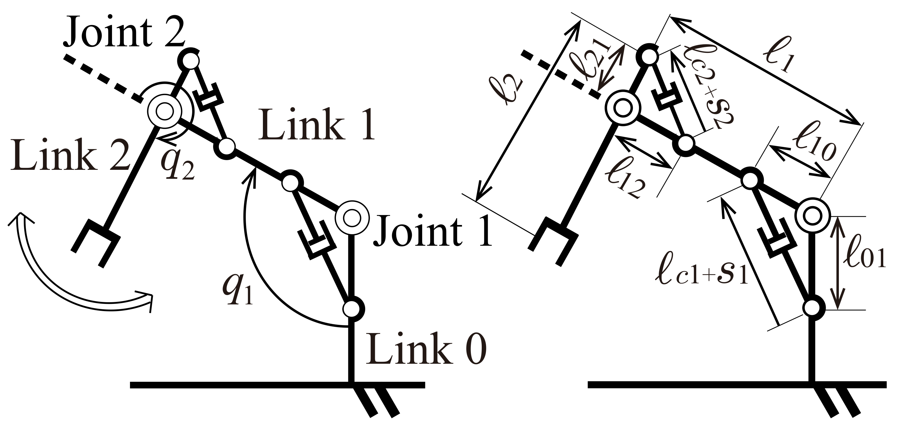
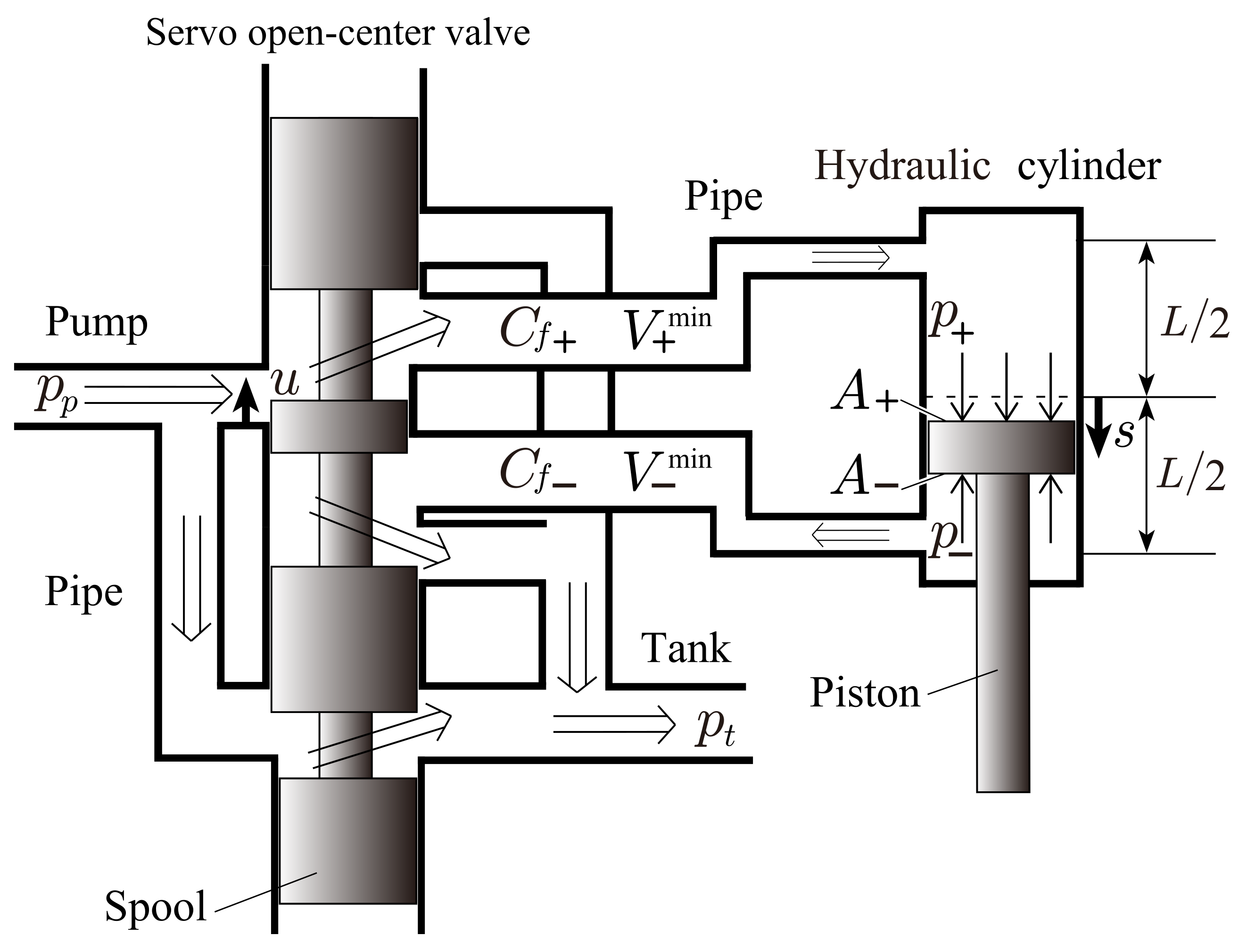
2. Nonlinear Nominal Model

Section 6 Let us consider a hydraulic arm whose nonlinear nominal model of Figure 1 and Figure 2 is a coupling of the hydraulic cylinder dynamics [18] and a pump pressure dynamics defined later. First, the hydraulic cylinder dynamics is described by
x ˙ = f 0 ( x ) + g 0 ( x ) u y = x
with
x = q 1 q 2 q ˙ 1 q ˙ 2 p + 1 p + 2 p 1 p 2 T , u = u 1 u 2 T
where the joint angle q i ( t ) (rad), the joint angle velocity q ˙ i ( t ) (rad/s), the cap side pressure p + i ( t ) (Pa), the rod side pressure p i ( t ) (Pa), and the orifice area (the input) u i ( t ) ( m 2 ) are the functions of time t [s]. The drift term f 0 ( x ) and the input term g o ( x ) u are defined as follows:
f 0 ( x ) = q ˙ 1 q ˙ 2 T J 1 ( q ) ( C ( q , q ˙ ) q ˙ + F d G ( q ) T s ˙ + F c G ( q ) T sgn ( s ˙ ) + g ( q ) G ( q ) T F ( x ) ) + F e f + 1 ( x ) f + 2 ( x ) T f 1 ( x ) f 2 ( x ) T g 0 ( x ) = O O g + 1 ( x ) 0 0 g + 2 ( x ) g 1 ( x ) 0 0 g 2 ( x )
J ( q ) = J 1 + 2 R 12 cos ( q 2 ) J 2 + R 12 cos ( q 2 ) J 2 + R 12 cos ( q 2 ) J 2 C ( q , q ˙ ) = 2 R 12 q ˙ 1 q ˙ 2 sin ( q 2 ) R 12 q ˙ 2 2 sin ( q 2 ) R 12 q ˙ 1 2 sin ( q 2 ) F d = F d 1 0 0 F d 2 , F c = F c 1 0 0 F c 2 g ( q ) = W 1 g sin ( q 1 ) + W 2 g sin ( q 1 + q 2 ) W 2 g sin ( q 1 + q 2 ) G ( q ) T = G 11 ( q 1 ) 0 0 G 22 ( q 2 ) F ( x ) = A + 1 p + 1 ( t ) A 1 p 1 ( t ) A + 2 p + 2 ( t ) A 2 p 2 ( t ) , F e = F e 1 F e 2 f + i ( x ) = b V + i ( s i ) A + i s ˙ i ( t ) C i i ( p + i ( t ) p i ( t ) ) C e + i p + i ( t ) f i ( x ) = b V i ( s i ) + A i s ˙ i ( t ) + C i i ( p + i ( t ) p i ( t ) ) C e i p i ( t ) g + i ( x ) = b V + i ( s i ) + C f + i h + i ( p + i , p p , p t ) g i ( x ) = b V i ( s i ) C f i h i ( p i , p p , p t ) J 1 = I 1 + I 2 + m 1 g 1 2 + m 2 1 2 + g 2 2 , J 2 = I 2 + m 2 g 2 2 R 12 = m 2 g 2 1 , W 1 = m 1 g 1 + m 2 1 , W 2 = m 2 g 2 G 11 = 01 10 sin ( q 1 ) c 1 + s 1 ( t ) , G 22 = 12 21 sin ( 2 π q 2 ) c 2 + s 2 ( t ) V + i ( s i ) = V + i min + L i / 2 + s i ( t ) A + i , V i ( s i ) = V i min + L i / 2 s i ( t ) A i h + i ( p + i , p p , p t ) = p + i ( t ) + p p ( t ) ( u i ( t ) > 0 ) 1 2 p p ( t ) 1 2 p t ( t ) ( u i ( t ) = 0 ) p + i ( t ) p t ( t ) ( u i ( t ) < 0 ) h i ( p i , p p , p t ) = p i ( t ) p t ( t ) ( u i ( t ) > 0 ) 1 2 p p ( t ) 1 2 p t ( t ) ( u i ( t ) = 0 ) p i ( t ) + p p ( t ) ( u i ( t ) < 0 )
where the subscript i = 1 or 2 is the joint number and the subscript + or − denotes the cap side and the rod side, respectively. The piston displacement s i ( t ) (m), the pump pressure p p ( t ) (Pa), and the tank pressure p t ( t ) (Pa) are the functions of time t (s). The cylinder Jacobian matrix G i i ( q i ) (m) is the function of the joint angle q i ( t ) (rad). The external force F e i is reaction force from the piston end walls. The physical parameters are the link mass m i (kg), the link moment of inertia around the center of the gravity I i ( k g · m 2 ), the stroke L i (m), the link length i (m), the distance between the joint center and the piston endpoint i j (m), the distance between the joint center and the center of the gravity g i (m), the piston minimal length c i (m), the piston areas A ± i ( m 2 ), the damping coefficient F d i ( N · s / m ), the Coulomb friction coefficient F c i (N), the gravity acceleration g ( m / s 2 ), the gravity coefficient W i ( m / s 2 ), the bulk modulus b (Pa), the flow gain coefficient C f ± i ( m / ( s · Pa ) ), the internal leakage coefficient C i i ( = C i 1 or C i 2 ) ( m 3 / ( s · Pa ) ), the external leakage coefficient C e ± i ( m 3 / ( s · Pa ) ), and the pipe volume V ± i min ( m 3 ). The nominal model introduces the restricted domain s i ( t ) ( L i / 2 , L i / 2 ) . The origin of the piston displacement s i ( t ) and the cylinder pressure p ± i ( t ) are the middle point of the stroke range, air pressure, respectively. C f + i h + i ( p + i , p p , p t ) and C f i h i ( p i , p p , p t ) are approximated by Bernoulli’s principle.
Second, the pump pressure dynamics are described by
p ˙ p ( t ) = b p V p Q p i = 1 2 Q i Q t
where the pump bulk modulus b p (Pa) and the pipe volume V p ( m 3 ) are the physical parameters. The pump flow rate Q p ( m 3 / s ) is the function of time. The input flow rate Q i ( m 3 / s ) and the tank flow rate Q t ( m 3 / s ) are approximated by Bernoulli’s principle as hydraulic cylinder dynamics:
Q i = C f + i h + i ( p + i , p p , p t ) u i ( t ) 1 + sgn ( + u i ( t ) ) 2 + C f i h i ( p i , p p , p t ) u i ( t ) 1 sgn ( + u i ( t ) ) 2 Q t = C f t h t ( p p , p t ) 1 i = 1 2 1 / ( u i m a x u i ( t ) ) 2 u s u m ( t )
with
h t ( p p , p t ) = p p ( t ) p t ( t )
where the tank flow coefficient C f t ( m / ( s · Pa ) ) and the maximum orifice area u i m a x ( m 2 ) are the physical parameters.
Remark 1.
The nonlinear nominal model in Equation (1) ignores the piston mass, the cylinder mass (cf. [4]), and the nonlinear friction effect at least. Equation (2) assumes the steady flow and the negligible servo dynamics of an open-center valve [25,26]. See [18] for more details of the nonlinear nominal model.

3. Physical Parameter Identification

In this section, we update our previous physical parameter identification method [20,21] for agriculture scale excavators with open-center valves. The previous method cannot be applicable to any open-center valves but the updated method is applicable to closed-center valves as a special case. More precisely, the updated method can discuss the pump pressure dynamics as well as the hydraulic cylinder dynamics. In the rest of this paper, just for simplicity, without loss of generality, we show only the case of joint 2 as shown in Figure 3.

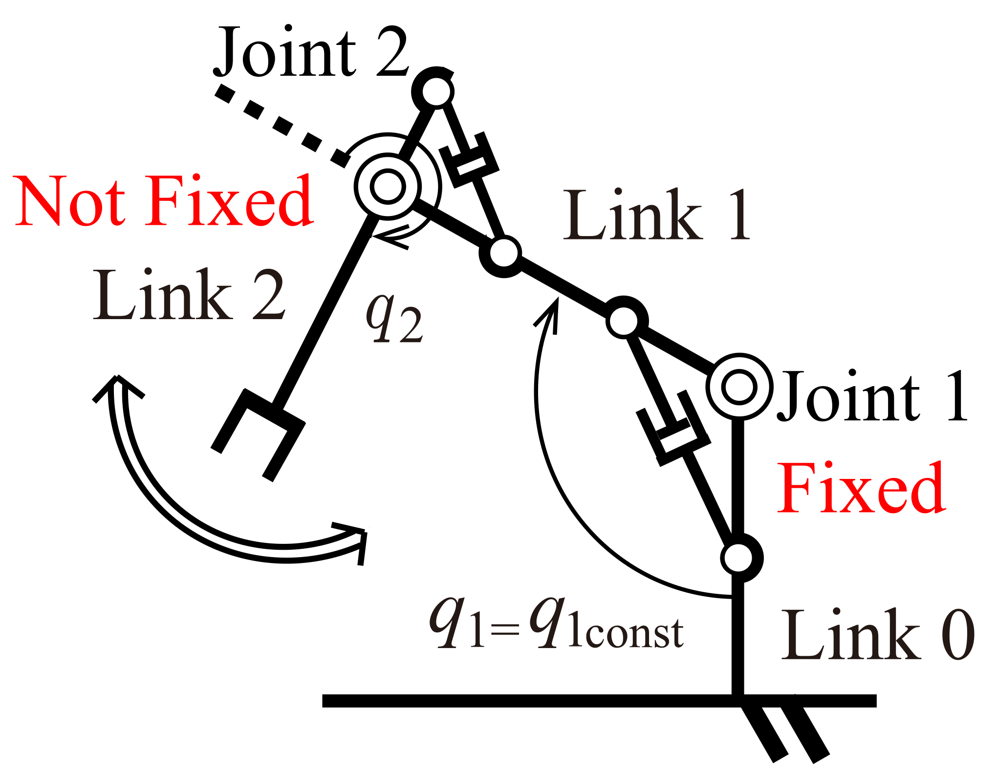
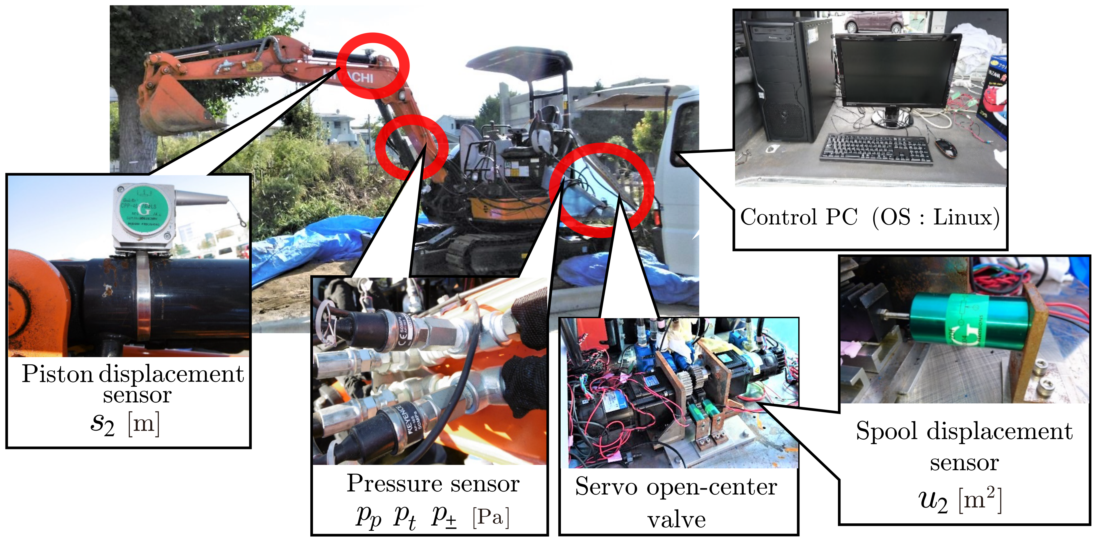
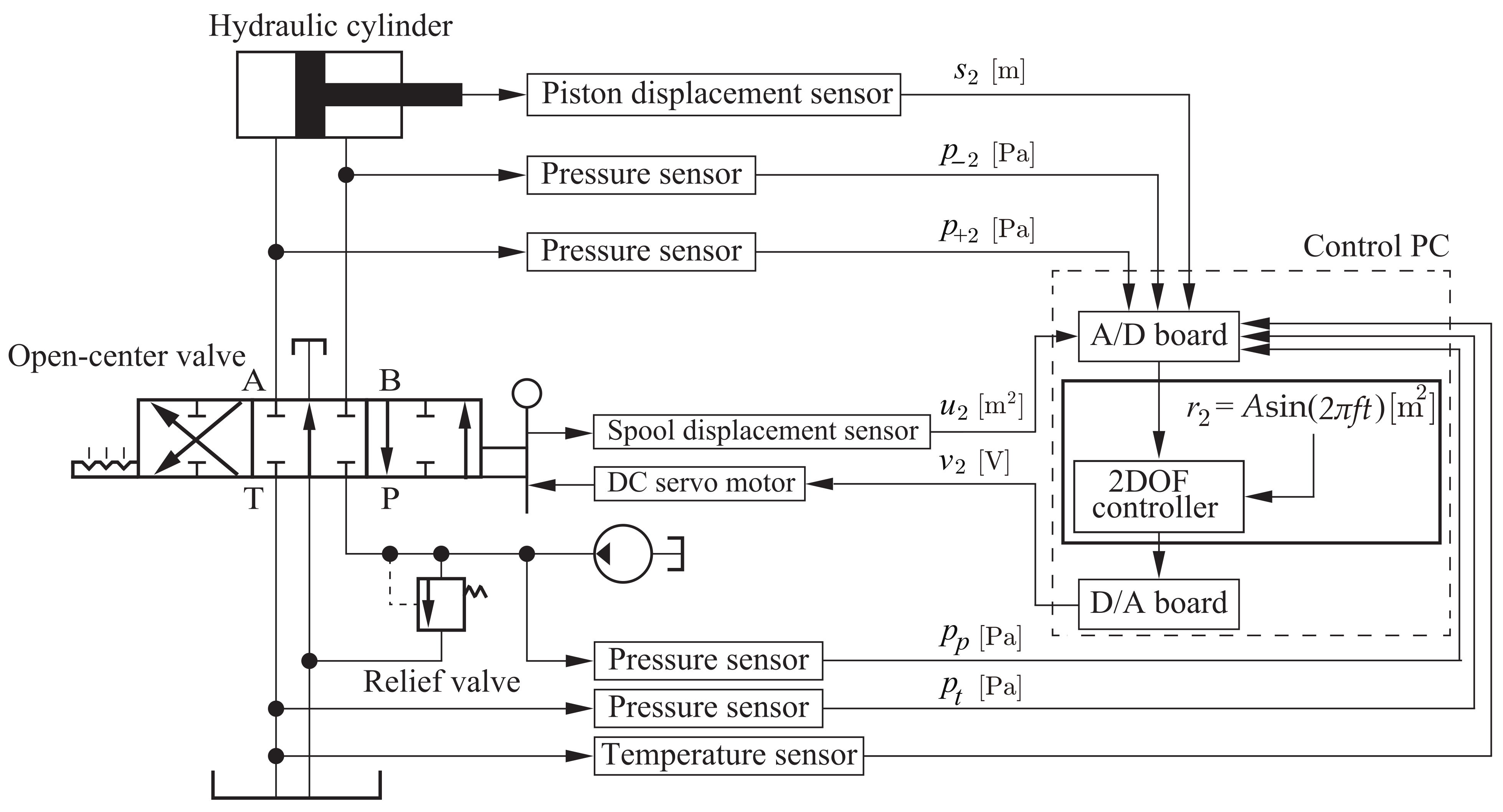
3.1. Experimental Condition (Identification)

From Equations (1) and (2), the equations of motion for the mechanical and the continuity equations for fluid systems are as follows:
J 2 q ¨ 2 ( t ) + G 22 ( q 2 ( t ) ) F d 2 s ˙ 2 ( t ) + G 22 ( q 2 ( t ) ) F c 2 sgn ( s ˙ 2 ( t ) ) + W 2 g sin ( q 1 const + q 2 ( t ) ) = G 22 ( q 2 ( t ) ) A + 2 p + 2 ( t ) A 2 p 2 ( t )
and
p ˙ + 2 ( t ) = b V + 2 ( s 2 ) A + 2 s ˙ 2 ( t ) C i 2 ( p + 2 ( t ) p 2 ( t ) ) C e + 2 p + 2 ( t ) + C f + 2 h + 2 u 2 ( t ) p ˙ 2 ( t ) = b V 2 ( s 2 ) + A 2 s ˙ 2 ( t ) + C i 2 ( p + 2 ( t ) p 2 ( t ) ) C e 2 p 2 ( t ) C f 2 h 2 u 2 ( t ) p ˙ p ( t ) = b p V p ( Q p C f + 2 h + 2 u 2 ( t ) 1 + sgn ( + u 2 ( t ) ) 2 C f 2 h 2 u 2 ( t ) 1 sgn ( + u 2 ( t ) ) 2 C f t h t u sum ( t ) ) .
<STEP1> It is possible to see that Equations (4) and (5) can be linear equations with respect to the unknown physical parameters.
Equation (4) ⇒
σ 11 ( t 1 ) σ 12 ( t 1 ) σ 13 ( t 1 ) σ 14 ( t 1 ) σ 11 ( t N ) σ 12 ( t N ) σ 13 ( t N ) σ 14 ( t N ) X 1 N J 2 F d 2 F c 2 W 2 a 1 = f 11 ( t 1 ) f 11 ( t N ) Y 1 N
with
σ 11 ( t ) = q ¨ 2 ( t ) , σ 12 ( t ) = G 22 ( q 2 ) s ˙ 2 ( t ) , σ 13 ( t ) = G 22 ( q 2 ) sgn ( s ˙ 2 ) σ 14 ( t ) = g sin ( q 1 const + q 2 ) , f 11 ( t ) = G 22 ( q 2 ) A + 2 p + 2 ( t ) A 2 p 2 ( t )
and Equation (5) ⇒
ϵ 11 ( t 1 ) 0 ϵ 13 ( t 1 ) 0 0 ϵ 16 ( t 1 ) 0 ϵ 18 ( t 1 ) ϵ 21 ( t 1 ) 0 0 ϵ 24 ( t 1 ) 0 0 ϵ 27 ( t 1 ) ϵ 28 ( t 1 ) 0 ϵ 32 ( t 1 ) ϵ 33 ( t 1 ) ϵ 34 ( t 1 ) ϵ 35 ( t 1 ) 0 0 0 ϵ 11 ( t N ) 0 ϵ 13 ( t N ) 0 0 ϵ 16 ( t N ) 0 ϵ 18 ( t N ) ϵ 21 ( t N ) 0 0 ϵ 24 ( t N ) 0 0 ϵ 27 ( t N ) ϵ 28 ( t N ) 0 ϵ 32 ( t N ) ϵ 33 ( t N ) ϵ 34 ( t N ) ϵ 35 ( t N ) 0 0 0 X 2 N 1 / b 1 / b p C f + 2 C f 2 C ft C e + 2 C e 2 C i 2 a 2 = f 21 ( t 1 ) f 22 ( t 1 ) f 23 ( t 1 ) f 21 ( t N ) f 22 ( t N ) f 23 ( t N ) Y 2 N
with
ϵ 11 ( t ) = V + 2 ( t ) p ˙ + 2 ( t ) , ϵ 16 ( t ) = p + 2 ( t ) ϵ 13 ( t ) = + h + 2 u 2 ( t ) , ϵ 18 ( t ) = ( p + 2 ( t ) p 2 ( t ) ) ϵ 21 ( t ) = V 2 ( t ) p ˙ 2 ( t ) , ϵ 27 ( t ) = p 2 ( t ) ϵ 24 ( t ) = h 2 u 2 ( t ) , ϵ 28 ( t ) = + ( p + 2 ( t ) p 2 ( t ) ) ϵ 32 ( t ) = V p p ˙ p ( t ) , ϵ 33 ( t ) = + h + 2 u 2 ( t ) 1 + sgn ( + u 2 ( t ) ) 2 ϵ 35 ( t ) = h t u sum ( t ) , ϵ 34 ( t ) = + h 2 u 2 ( t ) 1 sgn ( + u 2 ( t ) ) 2 f 21 ( t ) = + A + 2 s ˙ 2 ( t ) , f 22 ( t ) = A 2 s ˙ 2 ( t ) f 23 ( t ) = + Q p
Note that the right-hand sides are not zero and known.
<STEP2> Suppose that [ q 2 ( t ) , q ˙ 2 ( t ) , q ¨ 2 ( t ) , p ± 2 ( t ) , p ˙ ± 2 ( t ) , p p ( t ) , p ˙ p ( t ) , p t ( t ) , u 2 ( t ) ] is obtained at each time t = t 1 , , t N . From the project theorem in Hilbert space [27], the set of the unknown physical parameter a 1 and a 2 in Equations (6) and (7) are identified uniquely as the following values:
a ^ 1 = X 1 N T X 1 N 1 X 1 N T Y 1 N , a ^ 2 = X 2 N T X 2 N 1 X 2 N T Y 2 N .
Remark 2.
Apparently the obtained equation is similar to that in our previous paper [20,21]. However, as stated above, the pump pressure dynamics are not counted in the previous paper but are taken into account in this paper only. In this sense, the above method in the paper is updated from the previous method.
Figure 4 shows an appearance of the experimental setup. The experimental setup consists of an agricultural scale excavator (HITACHI, ZX30U-5A), pipes (BRIDGESTONE, PFH06, 3/8 inch), and a servo open-center valve only. In the paper, the second joint of the excavator is focused precisely. The excavator is driven by the servo open-center valve of Figure 5 whose orifice area u 2 is measured by a displacement sensor (MIDORI PRECISIONS, LP-20F) and a DC servo motor (SANYO, T720-0.12EL8, 0.2 kW), a rack and a pinion (reduction ratio 1/25), an AD board (interface, PCI-3155, 16 bit), a control PC (Linux, 3.8 GHz, 4.0 GB) [28], and a DA board (interface, PCI-3325, 12 bit). In the control PC, a 2DOF local controller is designed and implemented to make the orifice area u 2 into the actual control input against the large overlapping in the valve. The open-center valve has a direct relief valve. The outputs of the excavator are a piston displacement s 2 ( t ) measured by a piston displacement sensor (MIDORI PRECISIONS, CPP-45-150LS), the cap, rod, pump, and tank pressures p + 2 ( t ) , p 2 ( t ) , p p ( t ) , and p t ( t ) measured by the pressure sensors (KEYENCE, AP-16S) and the oil temperature measured by a thermocouple (NIHONDENSOKU, TNI-3.2-10-EXA4M). The oil temperature is 27 C. Figure 6 shows the system configuration in which an ideal sinusoidal signal r 2 and a control input v 2 to the DC servo motor. Table 1 shows the value of the known physical parameters before the physical parameter identification.
Since the physical parameter identification is in the off-line case, the time derivative of the piston displacement s ˙ 2 ( t ) and the cap and rod sides’ pressures p ˙ ± 2 ( t ) are sufficiently estimated via the first difference approximation and the standard moving average (43-order). In order to identify the physical parameters, the ideal sinusoidal signal r 2 ( t ) = 100 sin ( 2 π 0.5 t ) ( m 2 ) is applied and we cannot provide slower cases any more because the piston collides with the cylinder ends. The maximum input u 1 m a x and u 2 m a x is not used in the experiment.

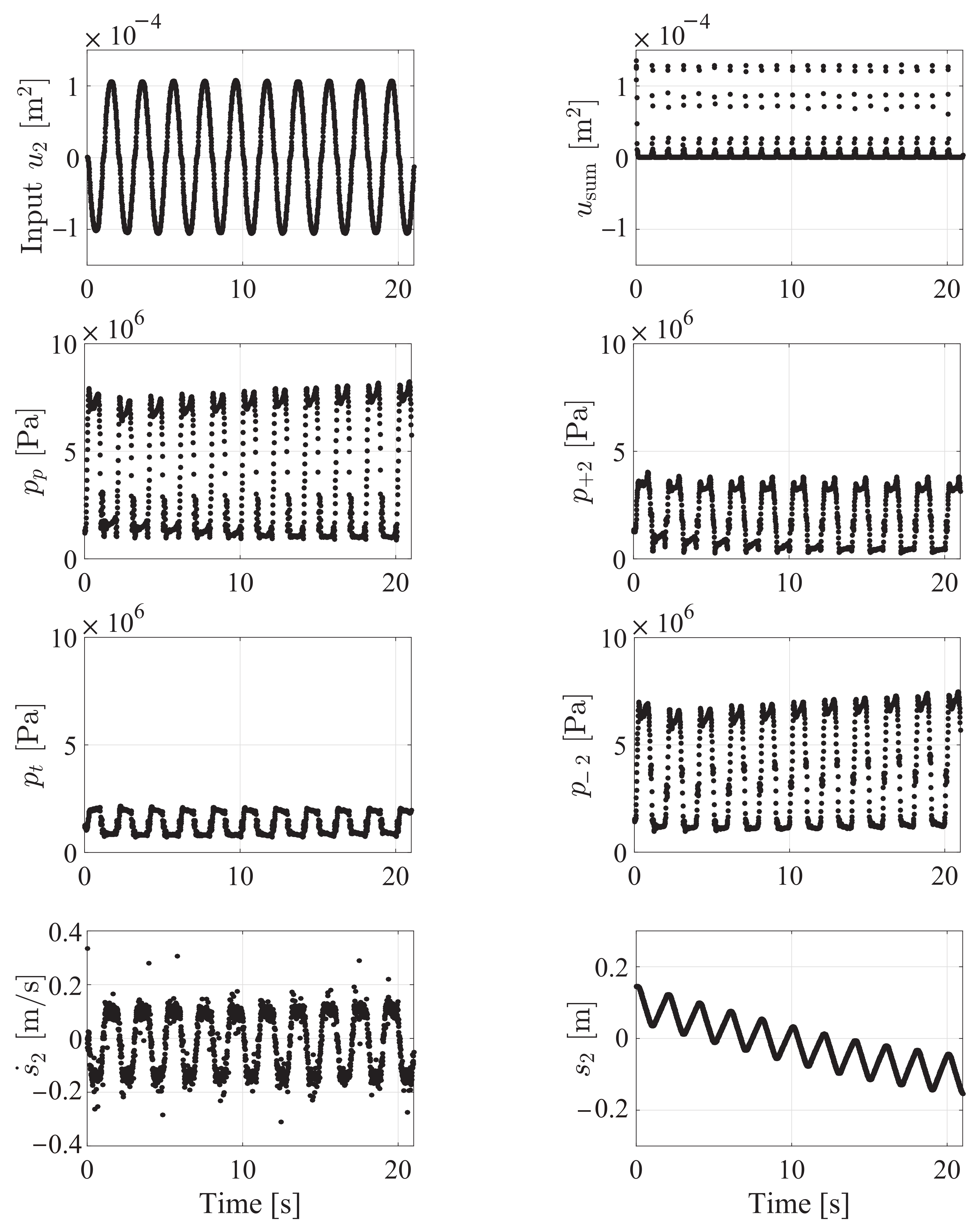
3.2. Experimental Results and Discussion (Identification)
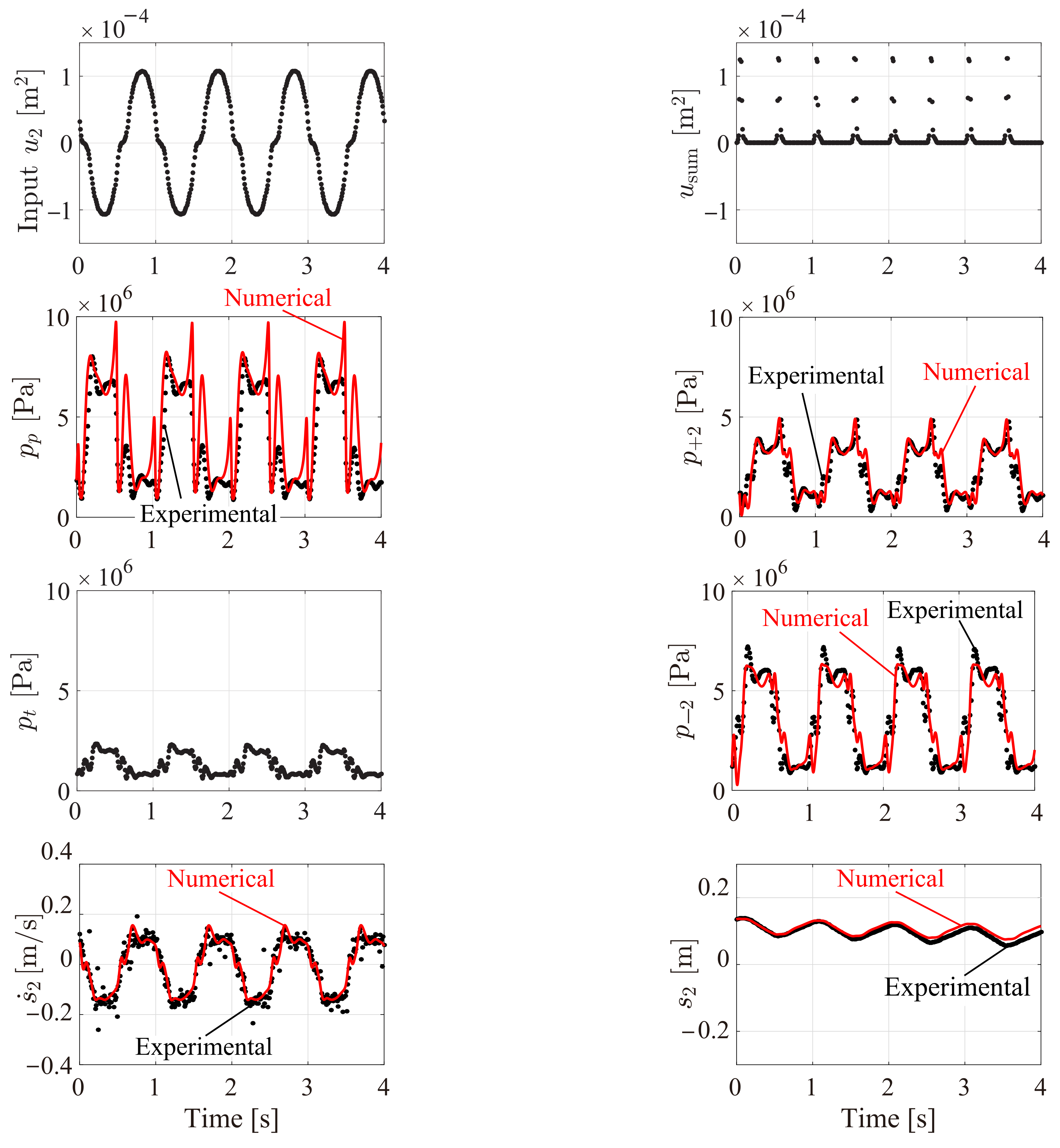
Figure 7 shows the experimental results from the ideal sinusoidal signal r 2 ( t ) = 100 sin ( 2 π 0.5 t ) ( m 2 ). The input u 2 was not equal to the ideal sinusoidal signal r 2 around the zero mark. This is due to the large overlapping. However, except for this overlapping effect, the input u 2 was equal to the almost sinusoidal signal r 2 . The time responses of the pressures and the piston displacement p + 2 ( t ) , p 2 ( t ) , p p ( t ) , p t ( t ) , and s 2 ( t ) were measured and the time responses of the piston velocity s 0 ( t ) ˙ was estimated. According to the input u 2 , every output responded sufficiently. The resolution and ranges of all sensors have no problems. In these senses, against actual noise and disturbances, the experimental setup is precisely justified to analyze the hydraulic cylinder dynamics on the agriculture scale instead of the laboratory scale. The relief valve did not work and the pressures did not saturate.
Table 2 shows the result of the physical parameter identification. In spite of the fact that the proposed method does not impose any restrictions on the sign or value range of the parameters and does not require any initial estimates of the parameters, all the identified physical parameter values were positive. The condition numbers of X 1 N were 26 and 220 where the number of the row was 17,500. The condition numbers were sufficiently small in this experiment.

4. Cross Validation

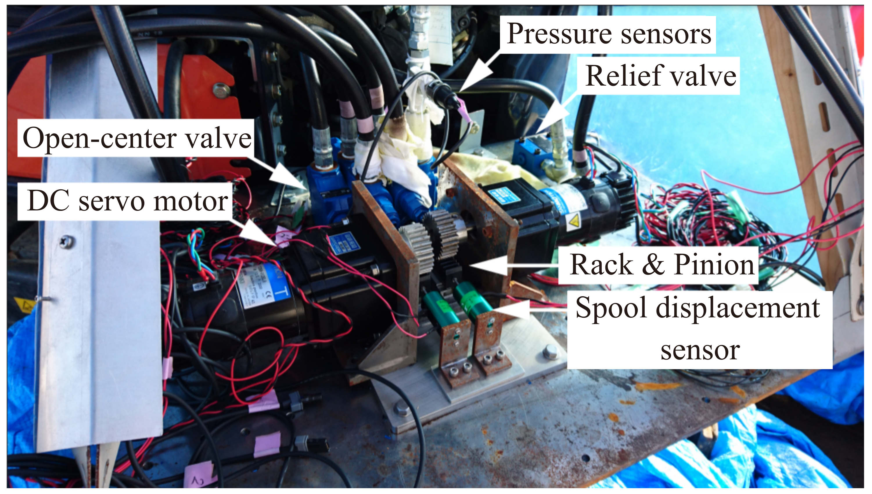
4.1. Experimental and Numerical Condition (Cross Validation)

First, the nominal numerical simulator is constructed with the physical parameters in Table 2 on the laptop (2.2 GHz, 4.0 GB, MATLAB R2015a, Simulink. Second, by the well-known Adams–Bashforth method (ode113) the numerical outputs are generated by an experimental input u 2 ( t ) that is never used in the physical parameter identification in Section 3. Third, the experimental outputs and the corresponding numerical outputs are generated by the same experimental input and are compared with each other. In order to discuss the model validation, the ideal sinusoidal signal r 2 ( t ) = 100 sin ( 2 π 1.0 t ) ( m 2 ) is applied and we cannot provide faster cases any more because not only the cylinders but also the whole hydraulic machinery is vibrated. Note that, in general, a frequency to discuss the model validation should be different from a frequency to identify the physical parameters and also should be higher to investigate the modeling error or uncertainty. Here the initial state values of the nominal numerical simulator are given from the measured values except the initial piston velocity s ˙ 2 ( 0 ) , which is not measured but estimated by just first order differentiation.

4.2. Experimental and Numerical Results and Discussion (Cross Validation)

Figure 8 shows the results of the cross validation. The black dots denote the experimental input and outputs from the experimental excavator. The red lines denote the numerical outputs from the nominal numerical simulator. In this section, we compare the experimental outputs and numerical outputs via the fit ratio [29]:
FIT : = 1 ( y ( k ) y ^ ( k ) ) 2 ( y ( k ) E [ y ( k ) ] ) 2 × 100
where y is the output of the experimental excavator, y ^ is the output of the nominal numerical simulator, and E [ x ] is the average value of x. Table 3 shows the fit ratio. Every ratio was positive, though a fit ratio can be negative very easily in general. As mentioned in Section 3, the pump pressure dynamics are not discussed in the previous paper [20,21]. In Figure 8, successfully, the output of the pump pressure from the experimental excavator and that from the nominal numerical simulator were close to each other. The amplitude errors can be observed but the phase and the number of the peaks were very similar. From a model-based control viewpoint, the phase-delay matching is often more important than the gain matching. Against modeling errors, not only the cap and rod sides pressures p + 2 ( t ) and p 2 ( t ) but also the pump pressure p p ( t ) are generated sufficiently. One of the guidelines of the acceptable modeling error is a phase delay condition. From the viewpoint of the passivity [9,11] by which port-Hamiltonian systems can achieve the large region of attraction, the phase delay between the experimental and numerical outputs should be less than 90 degrees. In Figure 8, the maximum phase delay of the model was 33.5 degrees in the rod pressure. In this sense, the modeling error is acceptable.

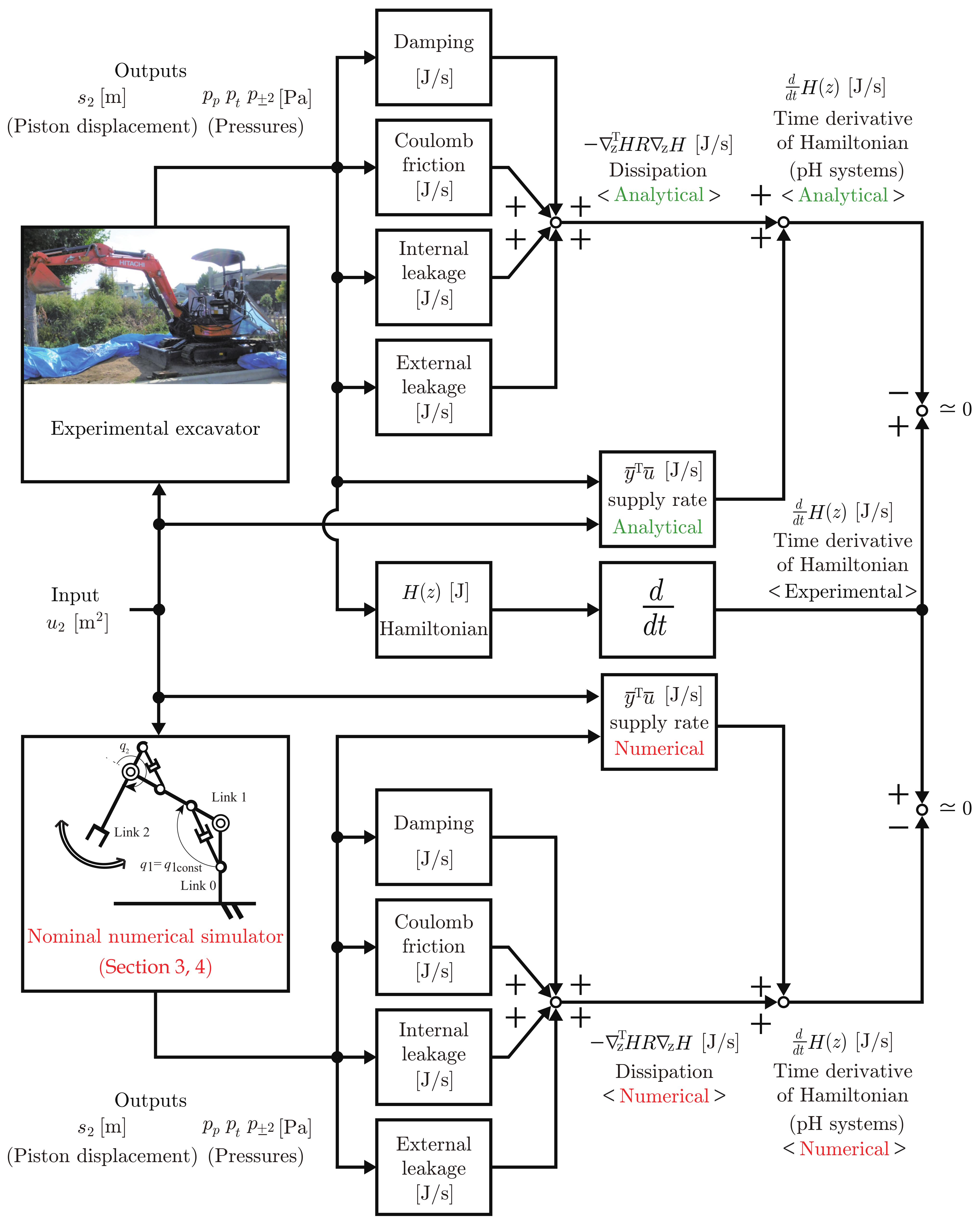
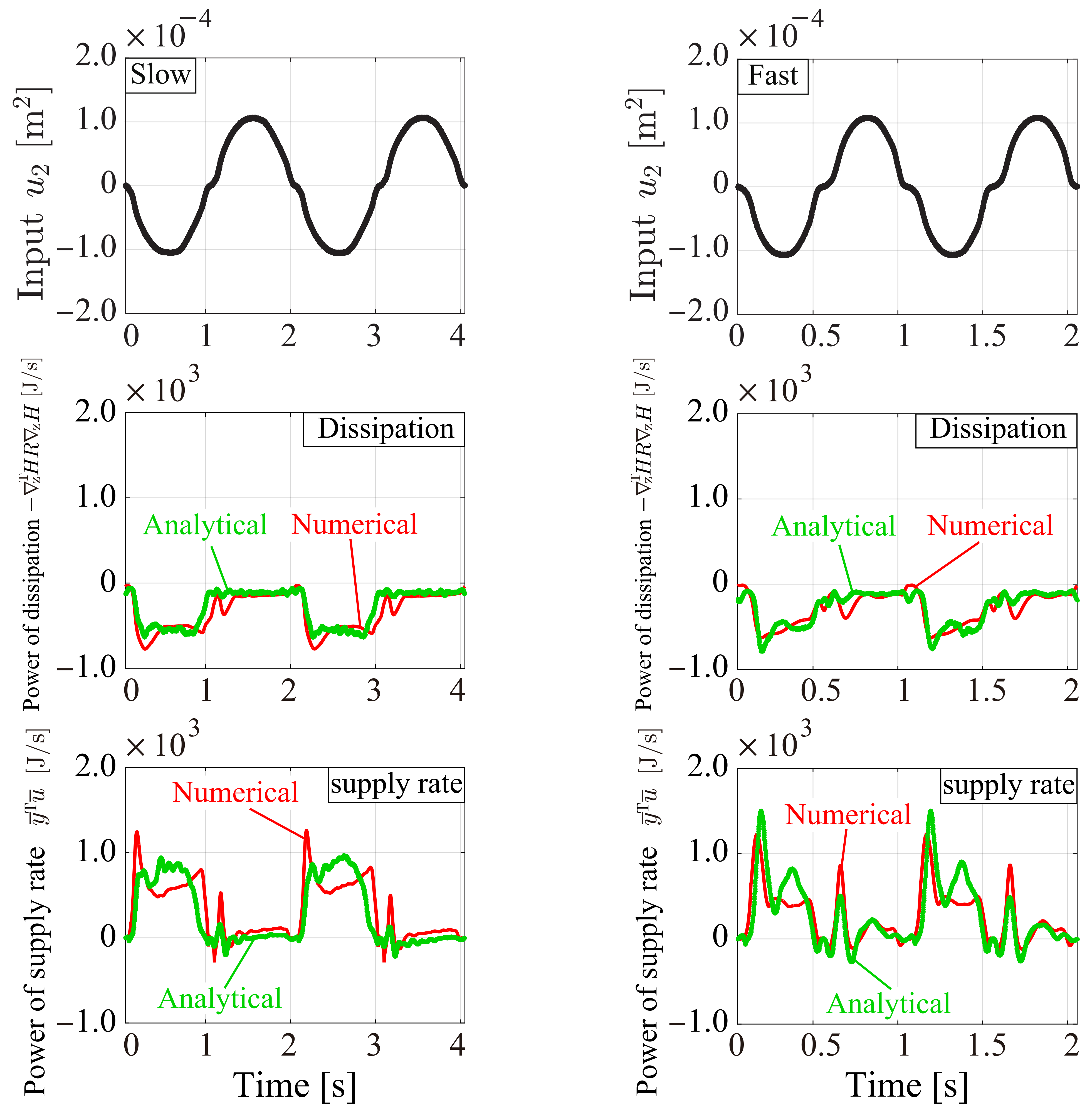
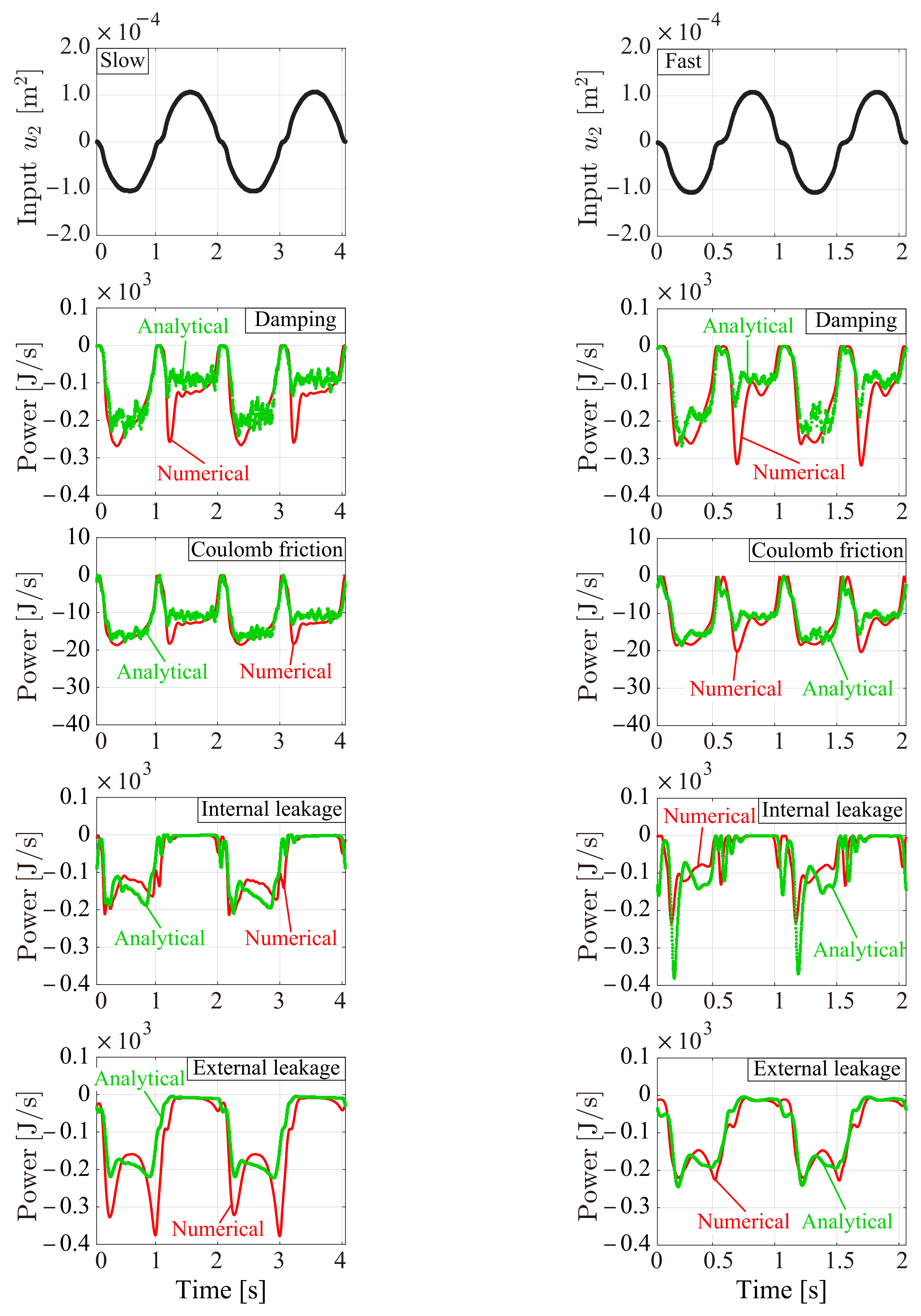
5. Energy Behavior Analysis

In this section we discuss the analytical, experimental, and numerical energy behaviors of the excavator on the agricultural scale. First, we review the port-Hamiltonian system and apply the port-Hamiltonian system to the experimental excavator. In particular, we derive the time derivative of the Hamiltonian analytically. Second, the analytical, experimental, and numerical energy behaviors from the port-Hamiltonian point of view in agriculture scale are compared.

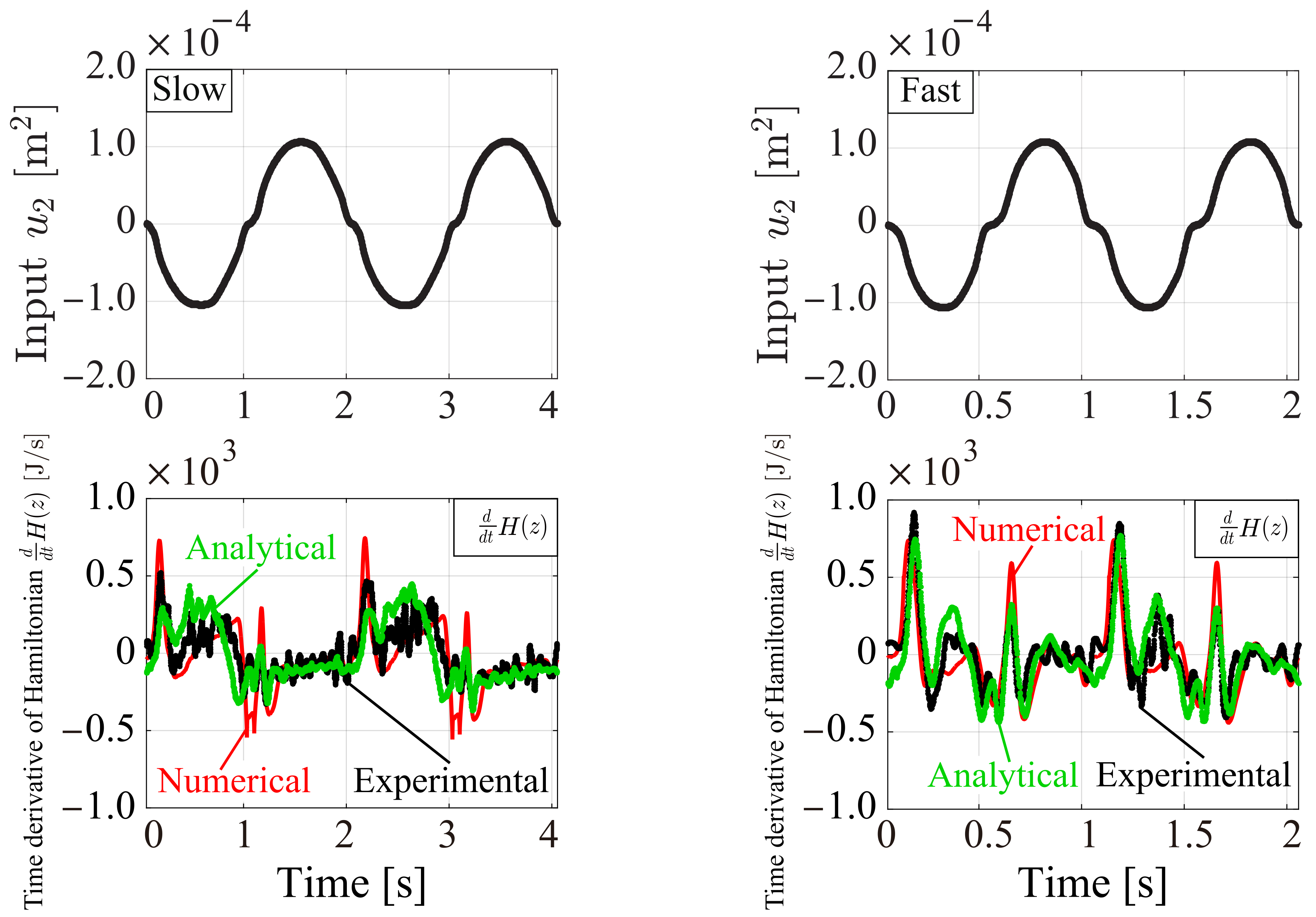
5.1. Analytical, Experimental, and Numerical Condition (Energy Behavior Analysis)

Let us review the port-Hamiltonian system. One of the most famous representations is the following input-state–output representation [9,10]:
z ˙ = J ( z ) R ( z ) z H ( z ) + g ( z ) u ¯ y ¯ = g ( z ) T z H ( z )
where z R n is the state, u ¯ R m is the input and y ¯ R m is the corresponding output. J ( z ) = J T ( z ) R n × n is a skew symmetric matrix and R ( z ) = R T ( z ) R n × n is a symmetric matrix. The notation z is the partial derivative with respect to z. In case of hydraulic cylinder dynamics, z, u ¯ , J ( z ) , R ( z ) , g ( z ) , and H ( z ) are given as:
z = q 2 q ˙ 2 p + 2 p 2 T , u ¯ = u 2
J ( z ) = 0 + 1 J 2 0 0 1 J 2 0 + 1 J 2 b A + 2 V + 2 ( s 2 ) G 22 1 J 2 b A 2 V 2 ( s 2 ) G 22 0 1 J 2 b A + 2 V + 2 ( s 2 ) G 22 0 0 0 + 1 J 2 b A 2 V 2 ( s 2 ) G 22 0 0
R ( z ) = 0 0 0 0 0 G 22 2 F d 2 q ˙ 2 + G 22 F c 2 sgn ( s ˙ 2 ) J 2 2 q ˙ 2 0 0 0 0 b C i 2 ( p 2 p + 2 ) C e + 2 p + 2 V + 2 ( s 2 ) ( 1 exp ( p + 2 b ) ) 0 0 0 0 b C i 2 ( p + 2 p 2 ) C e 2 p 2 V 2 ( s 2 ) ( 1 exp ( p 2 b ) ) g ( z ) = 0 0 + b C + 2 h + 2 V + 2 ( s ) b C 2 h 2 V 2 ( s )
and
H ( z ) = 1 2 J 2 q ˙ 2 2 W 2 g cos ( q 1 c o n s t + q 2 ) + V + 2 ( s 2 ) b exp p + 2 b 1 p + 2 + V 2 ( s 2 ) b exp p 2 b 1 p 2
which is one of the Hamiltonians and not unique due to the existence of the Casimir function cite [12,13]. For the Hamiltonian in the paper, the first term is the kinetic energy. The second term is the potential energy. The third and fourth terms are the internal energy. This choice of the Hamiltonian is meaningful from a class of model-based control of view [9,10,13,30,31]. The time derivative of the Hamiltonian H ˙ ( z ) is given as:
H ˙ ( z ) = z T H ( z ) z ˙ = z T H ( z ) ( J ( z ) R ( z ) ) z H ( z ) + g ( z ) u ¯ = z T H ( z ) J ( z ) z H ( z ) z T H ( z ) R ( z ) z H ( z ) + z T H ( z ) g ( z ) u ¯ = 0 z T H ( z ) R ( z ) z H ( z ) Dissipation + y ¯ T u ¯ . supply rate
The dissipation term and the supply rate term in the time derivative of the Hamiltonian z T H R z H and y ¯ T u ¯ are as follows:
z T H R z H Dissipation = q ˙ 2 2 G 22 2 F d 2 Damping q ˙ 2 G 22 2 F c 2 sgn ( q ˙ 2 ) Coulomb friction b C i 2 ( p + 2 p 2 ) exp p + 2 b exp p 2 b Internal leakage b C e + 2 p + 2 exp p + 2 b 1 b C e 2 p 2 exp p 2 b 1 External leakage
and
y ¯ T u ¯ supply rate = b C f + 2 h + 2 exp p + 2 b 1 b C f 2 h 2 exp p 2 b 1 u 2 .
Figure 9 shows the energy analysis procedure. First, we compare the analytical, experimental, and numerical energy behavior of the time derivative of the Hamiltonian. The analytical and numerical energy behaviors of the time derivative of the Hamiltonian are obtained indirectly by Equations (10)–(12), while the experimental energy behavior is derived directly from the measured Hamiltonian and its derivative. Second, we compare the analytical and numerical energy behaviors of the dissipation term and supply rate term. The analytical and numerical energy behaviors of the dissipation term and supply rate term are obtained by Equations (11) and (12), respectively. Finally, we compare the analytical and numerical energy behaviors of the damping term, Coulomb friction term, internal leakage term, and external leakage term in the dissipation term. The analytical and numerical energy behaviors of these four terms are obtained by Equation (11), respectively.
In the paper, we analyze the two cases, that is, the slowest case and the fastest case. In the slowest case, the control input u 2 has the frequency f = 0.5 [Hz]. In the fastest case, the control input u 2 has the frequency f = 1.0 [Hz].

5.2. Analytical, Experimental, and Numerical Results and Discussion (Energy Behavior Analysis)

Figure 10 shows the analytical, experimental, and numerical time responses of the time derivative of the Hamiltonian in the slow case and fast case. The analytical, experimental, and numerical energy behaviors were close to each other. One of the guidelines of the acceptable error is a phase delay condition. From the viewpoint of the passivity [9,11] by which port-Hamiltonian systems can achieve the large region of attraction; the phase delay between the analytical, experimental, and numerical outputs should be less than 90 degrees. In Figure 10, the maximum phase delay of the time derivative of Hamiltonian was 57.6 degrees. In this sense, the error is acceptable. One of the most important features is the asymmetric behaviors of the time derivative Hamiltonian. Note that the input u 2 is symmetric in the sense of the standard sinusoidal signal A sin ( 2 π f t ) . In our study, this asymmetrical behavior comes from the drift of the piston displacement s 2 ( t ) in Figure 7 and Figure 8. This drift is observed even in the absence of nonlinear frictions [18,32] and now observed experimentally in the presence of the actual frictions. In terms of energy, when the input u 2 is positive, the pump provides the cylinder with little energy to operate the piston, which is stored as internal energy in the fluid, and the piston is operated passively, mainly by converting the stored internal energy in the fluid into kinetic energy. Another important feature is the difference between the slow case and the fast case. This difference comes from the control limitation in the servo open-center valve to overcome the overlapping. In the period u 2 ≈ 0, the overlapping effect in the fast case is stronger than that in the slow case. This is the nature of the servo open-center valve.
Figure 11 shows the numerical and analytical time responses of the dissipation term and the supply rate term of the time derivative of the Hamiltonian. The numerical and analytical time responses of the dissipation term and the supply rate term were close to each other again. However, Figure 11 is valuable because the close behaviors in Figure 10 are just a necessary condition and not a sufficient condition for the close signals in Figure 11. Every response of the time derivative of the Hamiltonian in Figure 10 can be calculated only by the responses in Figure 11 but the opposite is also true. Indeed, it is observed that the main peak in Figure 10 in the fast case comes from the main peak in the supply rate and not from the dissipation. In addition, since the value of the input u 2 is less than 1.0 × 10 4 and also the values of part exp p ± 2 / b are almost 1 in our study, the peak in the supply rate comes from the pressure peak eventually.
Figure 12 shows the components of the time responses of the dissipation terms (the damping term, the Coulomb friction term, the internal leakage term, and the external leakage term). For every term, the numerical and analytical energy behaviors were close to each other again. Figure 12 is valuable because the close behaviors in the dissipation terms in Figure 11 are just a necessary condition and not a sufficient condition for the close behaviors in the four terms in Figure 12. Every response of dissipation in Figure 11 can be calculated only by the responses in Figure 12 but the opposite is also true. Indeed, except when the peaks in the supply rate are observed, the internal leakage as well as external leakage can be almost zero. These zeros correspond to the fact that these pressures are close to the tank pressure p t in our study. On the other hand, the Coulomb friction term is much smaller than the other three terms and the damping term strongly depends on the piston velocity causing the piston displacement s 2 ( t ) drift observed in Section 3 and Section 4. These observations in Figure 11 and Figure 12 support the results in Figure 10 eventually.
In all, via the analytical, experimental, and numerical energy behaviors, the applicability of the port-Hamiltonian theory is confirmed on the agricultural scale against modeling errors.

6. Conclusions

In this paper, a method for identifying physical parameters of an open-centered multi-degree-of-freedom hydraulic arm is proposed, and the effectiveness of the proposed method is verified by model validation and energy analysis for a one-DOF real construction machine arm. The pump pressure is formulated and a method to uniquely identify the unknown parameters of the open-centered hydraulic arm is given. The agreement between the nonlinear nominal model constructed by the identification and the output signal of the experimental excavator was confirmed under the experimental condition of different frequency from that of the identified input. In other words, we succeed in updating the physical parameter identification method to the pump pressure dynamics. The nominal model [20,21] based on many physical assumptions would be valid only in a limited scale range of time, length, mass and so on. On the other hand, the scale range in industrial excavators (e.g., a mini-shovel mining shovel) is not narrow and our scale is different from mining machines scale or the laboratory machines scale. It would be possible in future work to discuss such other scales. By calculating the output of the Hamiltonian, the validity of updating the model to the port-Hamiltonian system of an open-centered hydraulic arm was evaluated. In all, via the analytical, experimental, and numerical energy behaviors, the applicability of the port-Hamiltonian theory is confirmed in agriculture scale against modeling errors. Future work will be to verify the model and with simultaneous motion of two axes, and to analyze the energy.

Author Contributions

Conceptualization, R.A., S.S. and Q.Z.; methodology, R.A. and S.S.; software, R.A. and A.T.; validation, R.A. and A.T.; formal analysis, R.A. and S.S.; investigation, S.S. and A.T.; data curation, A.T.; writing—original draft preparation, R.A.; writing—review and editing, R.A. and S.S.; visualization, R.A. and A.T.; supervision, S.S.; project administration, S.S.; funding acquisition, S.S. All authors have read and agreed to the published version of the manuscript.

Funding

This research was partially funded by JSPS KAKENHI grant number 21K03934 and 26420173.

Institutional Review Board Statement

Not applicable.

Informed Consent Statement

Not applicable.

Acknowledgments

The authors are also grateful for the technical help provided by Yusuke Nabana, Yuki Nishimura, and Kazuki Nagai.

Conflicts of Interest

The authors declare no conflict of interest.

References

  1. Zhang, Q. Basics of HYDRAULIC SYSTEMS; Taylor & Francis: Abingdon, UK, 2008. [Google Scholar]
  2. Huang, Y.; Zhang, Q. Agricultural Cybernetics; Springer: Berlin/Heidelberg, Germany, 2021. [Google Scholar]
  3. Sakai, S.; Iida, M.; Osuka, K.; Umeda, M. Design and Control of a Heavy Material Handling Manipulator for Agricultural Robots. Auton. Robot. 2008, 25, 189–204. [Google Scholar] [CrossRef] [Green Version]
  4. Mattila, J.; Koivumaki, D.; Caldwell, D.G.; Semini, C. A survey on control of hydraulic robotic manipulators with projection to future trends. IEEE/ASME Trans. Mechatron. 2017, 22, 669–680. [Google Scholar] [CrossRef]
  5. Raibert, M.; Blankespoor, K.; Nelson, G.; Playter, R. BigDog, the Rough-Terrain Quadruped Robot. In Proceedings of the IFAC World Congress, Seul, Korea, 6–11 June 2008; pp. 10822–10825. [Google Scholar]
  6. Merritt, H. Hydraulic Control Systems; John Willey & Sons: Hoboken, NJ, USA, 1967. [Google Scholar]
  7. Watton, J. Fluid Power Systems; Springer: Englewood Cliffs, NJ, USA, 1989. [Google Scholar]
  8. Mohieddine, J.; Andreas, K. Hydraulic Servo-Systems; Springer: Berlin/Heidelberg, Germany, 2003. [Google Scholar]
  9. Duindam, V.; Macchelli, A.; Stramigioli, S.; Bruyninckx, H. Modeling and Control of Complex Physical Systems: The Port-Hamiltonian Approach; Springer: Berlin/Heidelberg, Germany, 2009. [Google Scholar]
  10. Van der Schaft, A.J. L2-Gain and Passivity Techniques in Nonlinear Control; Springer: Berlin/Heidelberg, Germany, 2000. [Google Scholar]
  11. Khalil, H. Nonlinear Systems; Prentice Hall: Hoboken, NJ, USA, 2002. [Google Scholar]
  12. Sakai, S. Fast Computation by Simplifications of a Class of Hydro-Mechanical Systems. In Proceedings of the IFAC Workshop on Lagrangian and Hamiltonian Methods for Nonlinear Control, Bertinoro, Italy, 29–31 August 2012; pp. 7–12. [Google Scholar]
  13. Kugi, A.; Kemmetmuller, W. New Energy-based Nonlinear Controller for Hydraulic Piston Actuators. Eur. J. Control 2004, 10, 163–173. [Google Scholar] [CrossRef]
  14. Nurmi, J.; Mattila, J. Global Energy-Optimal Redundancy Resolution of Hydraulic Manipulators: Experimental Results for a Forestry Manipulator. Energies 2017, 10, 647. [Google Scholar] [CrossRef] [Green Version]
  15. Vukovic, M.; Leifeld, R.; Murrenhoff, H. Reducing Fuel Consumption in Hydraulic Excavators—A Comprehensive Analysis. Energies 2017, 10, 687. [Google Scholar] [CrossRef] [Green Version]
  16. Lu, L.; Yao, B. Energy-Saving Adaptive Robust Control of a Hydraulic Manipulator Using Five Cartridge Valves With an Accumulator. IEEE Trans. Ind. Electron. 2014, 61, 7046–70548. [Google Scholar] [CrossRef]
  17. Abdel-Baqi, O.; Miller, P.; Nasiri, A. Energy Management for an 8000 hp Hybrid Hydraulic Mining Shovel. IEEE Trans. Ind. Appl. 2015, 1–8. [Google Scholar] [CrossRef]
  18. Sakai, S.; Stramigioli, S. Visualization of Hydraulic Cylinder Dynamics by a Structure Preserving Nondimensionalization. IEEE/Asme Int. Trans. Mechatron. 2018, 23, 2196–2206. [Google Scholar] [CrossRef]
  19. Morselli, R.; Zanasi, R.; Ferracin, P. Dynamic Model of an Electro-hydraulic Three Point Hitch. In Proceedings of the 2006 American Control Conference, Minneapolis, MN, USA, 14–16 June 2006. [Google Scholar] [CrossRef]
  20. Maeshima, Y.; Sakai, S.; Nakanishi, M.; Osuga, K. A Base Parameter Identification Method and Model Validation for Hydraulic Arms. J. JFPS 2012, 43, 16–21. [Google Scholar]
  21. Sakai, S.; Maeshima, Y. A New Method for Parameter Identification for N-DOF Hydraulic Robot. In Proceedings of the IEEE International Conference on Robotics and Automation (ICRA), Hong Kong, China, 31 May–5 June 2014; pp. 5983–5989. [Google Scholar]
  22. Saleem, A.; Kim, M.H. CFD Analysis on the Air-Side Thermal-Hydraulic Performance of Multi-Louvered Fin Heat Exchangers at Low Reynolds Numbers. Energies 2017, 10, 823. [Google Scholar] [CrossRef] [Green Version]
  23. Castilla, R.; Alemany, I.; Alger, A.; Javier Gamez-Montero, P.; Roquet, P.; Codina, E. Pressure-Drop Coefficients for Cushioning System of Hydraulic Cylinder With Grooved Piston: A Computational Fluid Dynamic Simulation. Energies 2017, 10, 1704. [Google Scholar] [CrossRef] [Green Version]
  24. Zardin, B.; Cillo, G.; Borghi, M.; D’Adamo, A.; Fontanesi, S. Pressure Losses in Multiple-Elbow Paths and in V-Bends of Hydraulic Manifolds. Energies 2017, 10, 788. [Google Scholar] [CrossRef] [Green Version]
  25. Li, Y.; Wang, Q. Pump-Pressure-Compensation-Based Adaptive Neural Torque Control of a Hydraulic Excavator with open-center Valves. In Proceedings of the IEEE/ASME International Conference on Advanced Intelligent Mechatronics (AIM), Auckland, NZ, USA, 9–12 July 2018; pp. 610–615. [Google Scholar]
  26. Tatsuoka, A.; Sakai, S.; Zhang, Q. Modeling of Hydraulic Robots with an Open-Center Dynamics. In Proceedings of the SICE ISCS, Kumamoto, Japan, 7–9 March 2019. [Google Scholar]
  27. Luenberger, D. Optimization by Vector Space Method; Wiley Interscience: Chichester, NY, USA, 1968. [Google Scholar]
  28. Sakai, S.; Osuka, K.; Umeda, M.; Maekawa, T.; Umeda, M. Robust Control Systems of a Heavy Material Handling Agricultural Robot: A Case Study for Initial Cost Problem. IEEE Trans. Control Syst. Technol. 2007, 15, 1038–1048. [Google Scholar] [CrossRef]
  29. Ljung, L. System Identification: Theory for the User; Prentice Hall: Hoboken, NJ, USA, 1999. [Google Scholar]
  30. Sakai, S. A Direct Teaching Control via Casimir of Force Sensorless Hydraulic Arms. In Proceedings of the IEEE/ASME International Conference on Advanced Intelligent Mechatronics, Hong Kong, China, 8–12 July 2019; pp. 211–216. [Google Scholar]
  31. Arai, R.; Sakai, S. A Verification Method of the Impedance Control Based on the Conserved Quantity for Symmetrical Hydraulic Arms. In Proceedings of the Conference of Japan Fluid Power System Society (JFPS), Okayama, Japan, 8–9 September 2020; pp. 54–56. (In Japanese). [Google Scholar]
  32. Richard, E.; Vivalda, J. Mathematical Analysis of Stability and Drift Behavior of Hydraulic Cylinders Driven by a Servovalve. ASME J. Dyn. Syst. Meas. Control 2002, 124, 206–213. [Google Scholar] [CrossRef]
Figure 1. Hydraulic arms.
Energies 14 06210 g001
Figure 2. A hydraulic cylinder, pipes, and an servo open-center valve (the joint number is reduced for simplicity).
Energies 14 06210 g002
Figure 3. Physical parameter identification motion (joint 1 is fixed and only joint 2 is driven (not fixed) without loss of generality).
Energies 14 06210 g003
Figure 4. Experimental setup.
Energies 14 06210 g004
Figure 5. Servo open-center valve.
Energies 14 06210 g005
Figure 6. System configuration.
Energies 14 06210 g006
Figure 7. Input u 2 and the outputs (identification, f = 0.5 [Hz], joint 2).
Energies 14 06210 g007
Figure 8. Input u 2 and the outputs (cross validation, f = 1.0 [Hz], joint 2).
Energies 14 06210 g008
Figure 9. Comparisons of experimental vs. numerical vs. analytical energy behaviors.
Energies 14 06210 g009
Figure 10. Experimental (black) vs. numerical (red) vs. analytical (green) time responses of the time derivative of the Hamiltonian. (Energy behavior analysis, slow: f = 0.5 [Hz], fast: f = 1.0 [Hz].)
Energies 14 06210 g010
Figure 11. Numerical (red) vs. analytical (green) time responses of the dissipation terms and supply rate terms of the time derivative of the Hamiltonian. (Energy behavior analysis, slow: f = 0.5 [Hz], fast: f = 1.0 [Hz].).
Energies 14 06210 g011
Figure 12. Numerical (red) vs. analytical (green) the components of the time responses of the dissipation term. (Energy behavior analysis, slow: f = 0.5 [Hz], fast: f = 1.0 [Hz].).
Energies 14 06210 g012
Table 1. Measured parameters and unknown parameters.
SymbolParameterValueUnit
J 2 Moment of inertiaUnknown kg · m 2
F d 2 Damping coefficientUnknown N · s / m
F c 2 Coulomb friction coefficientUnknown N
W 2 Gravity coefficientUnknown kg · m
g Gravity acceleration 9.8 m / s 2
2 Standard length of piston 1.5 m
c 2 Standard length of piston 2.8 × 10 1 m
12 Piston attachment position 1.1 m
21 Piston attachment position 3.3 × 10 1 m
L 2 Stroke 6.0 × 10 1 m
A + 2 Cap area 3.8 × 10 3 m 2
A 2 Rod area 2.6 × 10 3 m 2
b Bulk modulusUnknown MPa
b p Pump bulk modulusUnknown MPa
C f ± 2 Flow gainUnknown m / ( s · Pa )
C i 2 Internal leakage coefficientUnknown m 3 / ( s · Pa )
C e ± 2 External leakage coefficientUnknown m 3 / ( s · Pa )
C f t Tank flow gainUnknown m / ( s · Pa )
V + 2 min Cap pipe volume 3.4 × 10 4 m 3
V 2 min Rod pipe volume 3.0 × 10 4 m 3
V p Pump pipe volume 1.2 × 10 4 m 3
Q p Pump flow rate 3.8 × 10 4 m 3 / s
Table 2. Identification result for the nominal numerical simulator.
SymbolParameterValueUnit
J 2 Moment of inertia 2.3 × 10 2 kg · m 2
F d 2 Damping coefficient 1.3 × 10 4 N · s / m
F c 2 Coulomb friction coefficient 1.6 × 10 2 N
W 2 Gravity coefficient 1.9 × 10 2 kg · m
b Bulk modulus 9.6 × 10 8 Pa
b p Pump bulk modulus 6.5 × 10 7 Pa
C f + 2 Flow gain 4.6 × 10 3 m / ( s · Pa )
C f 2 Flow gain 4.0 × 10 3 m / ( s · Pa )
C i 2 Internal leakage coefficient 1.4 × 10 11 m 3 / ( s · Pa )
C e + 2 External leakage coefficient 4.1 × 10 12 m 3 / ( s · Pa )
C e 2 External leakage coefficient 3.0 × 10 12 m 3 / ( s · Pa )
C f t Tank flow gain 1.1 × 10 2 m / ( s · Pa )
Table 3. The result of cross validation (successfully the fit ratios are positive even though the fit ratio can easily be negative in general).
Pump pressure p p 33 > 0
Cap pressure p + 2 56 > 0
Rod pressure p 2 53 > 0
Piston velocity s ˙ 2 67 > 0
Piston displacement s 2 48 > 0
Publisher’s Note: MDPI stays neutral with regard to jurisdictional claims in published maps and institutional affiliations.

