
Geometry, Mesh and Numerical Scheme Influencing the Simulation of a Pelton Jet with the OpenFOAM Toolbox


Abstract
1. Introduction
2. Modelling
- being the averaged mixture velocity vector.
- p being the averaged mixture pressure.
- being the averaged mixture density computed as .
- g being the gravity acceleration.
- being the surface tension computed as with the surface tension (assumes constant), the local curvature of the interface and n the unit vector normal to the interface.
- being the mixture kinematic viscosity computed as .
- being the eddy viscosity computed using the SST model [23] that solves two additional transport equations for the turbulent kinetic energy k and the turbulent frequency .
- being the water volume fraction.
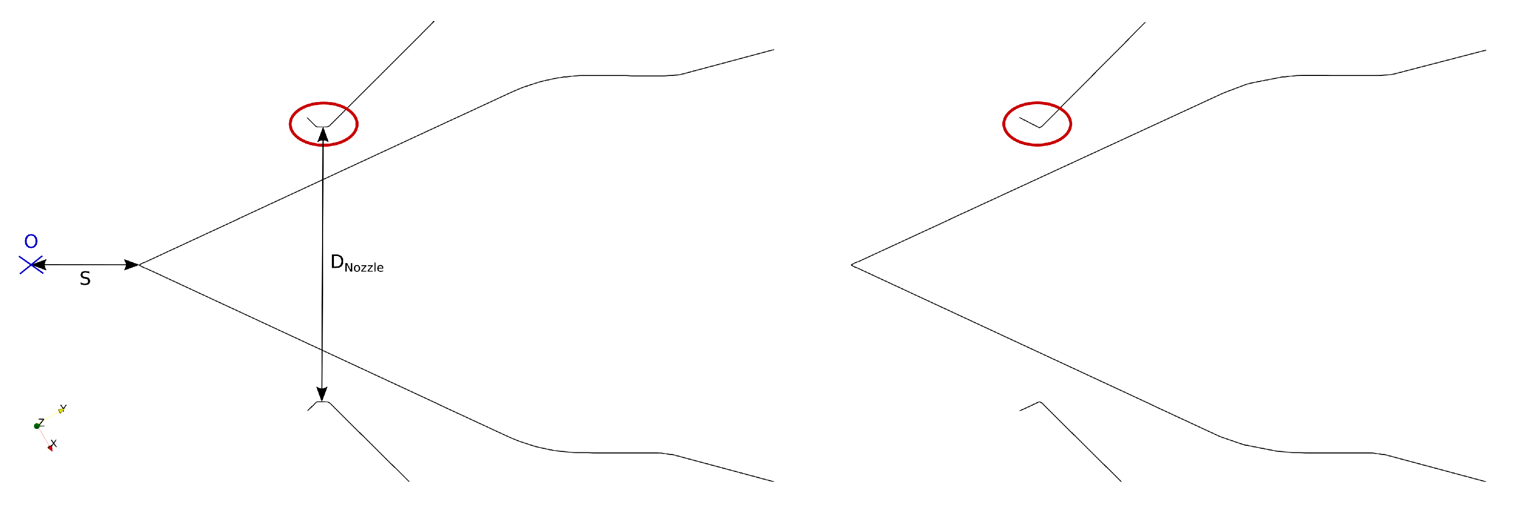
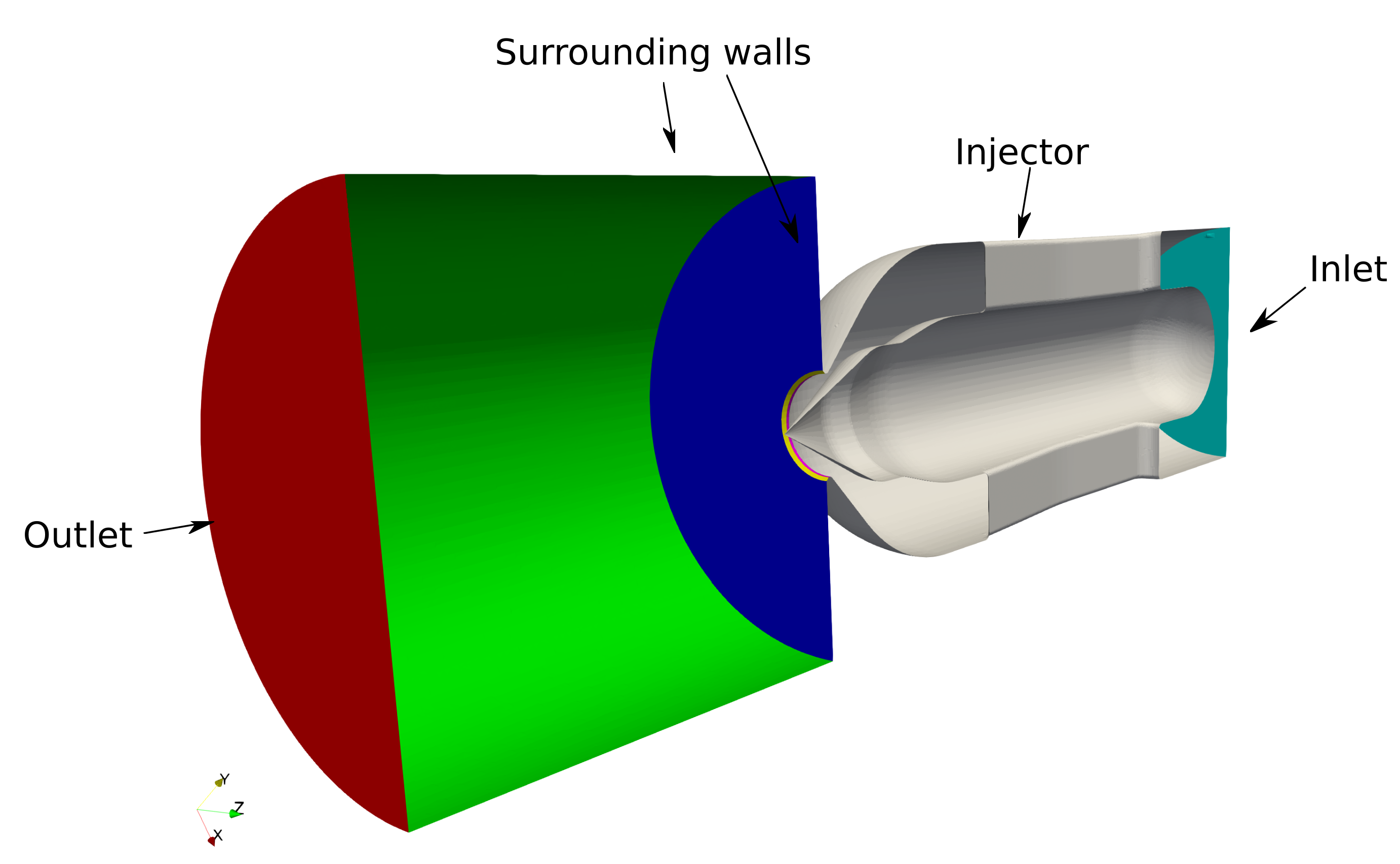
3. Geometry and Computational Domain
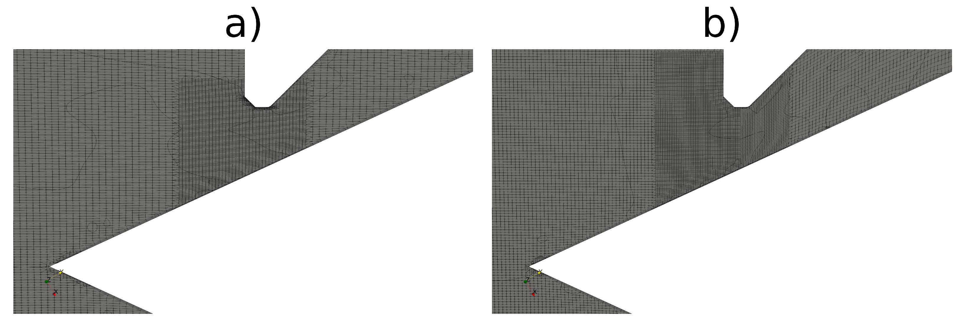
4. Mesh
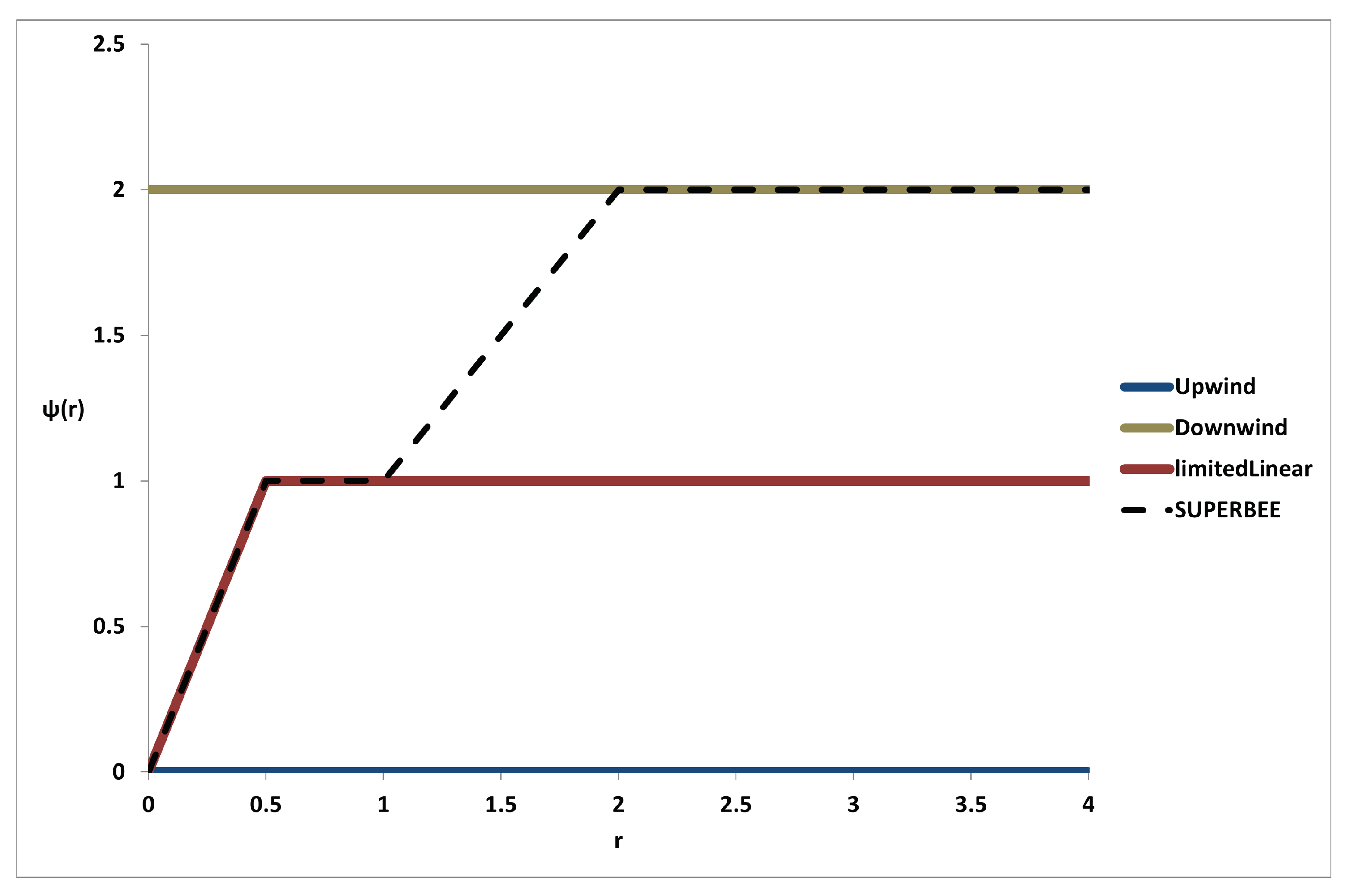
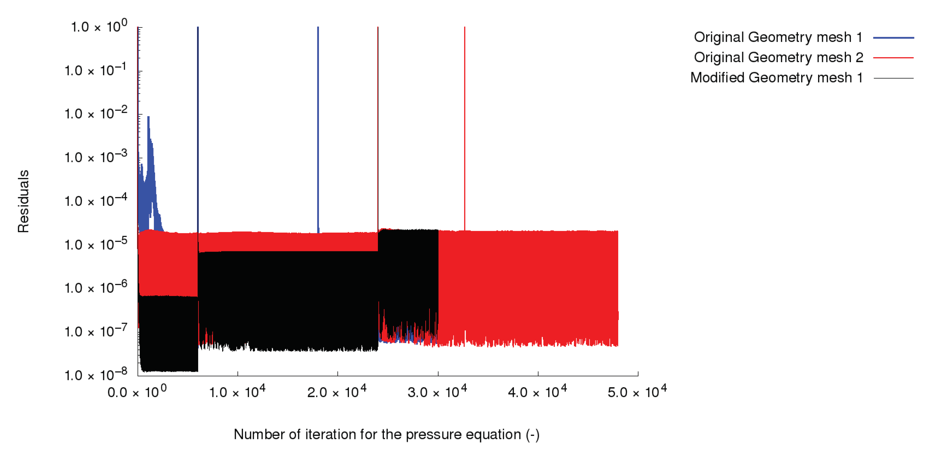
5. Numerical Setup
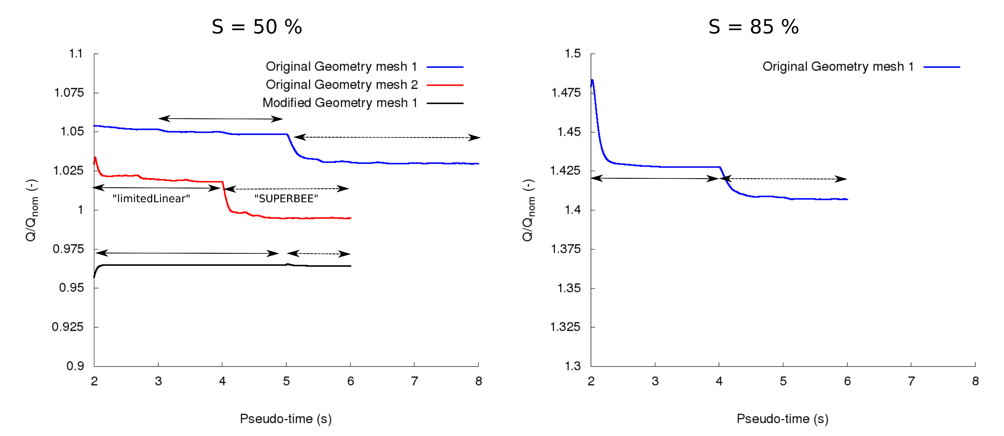
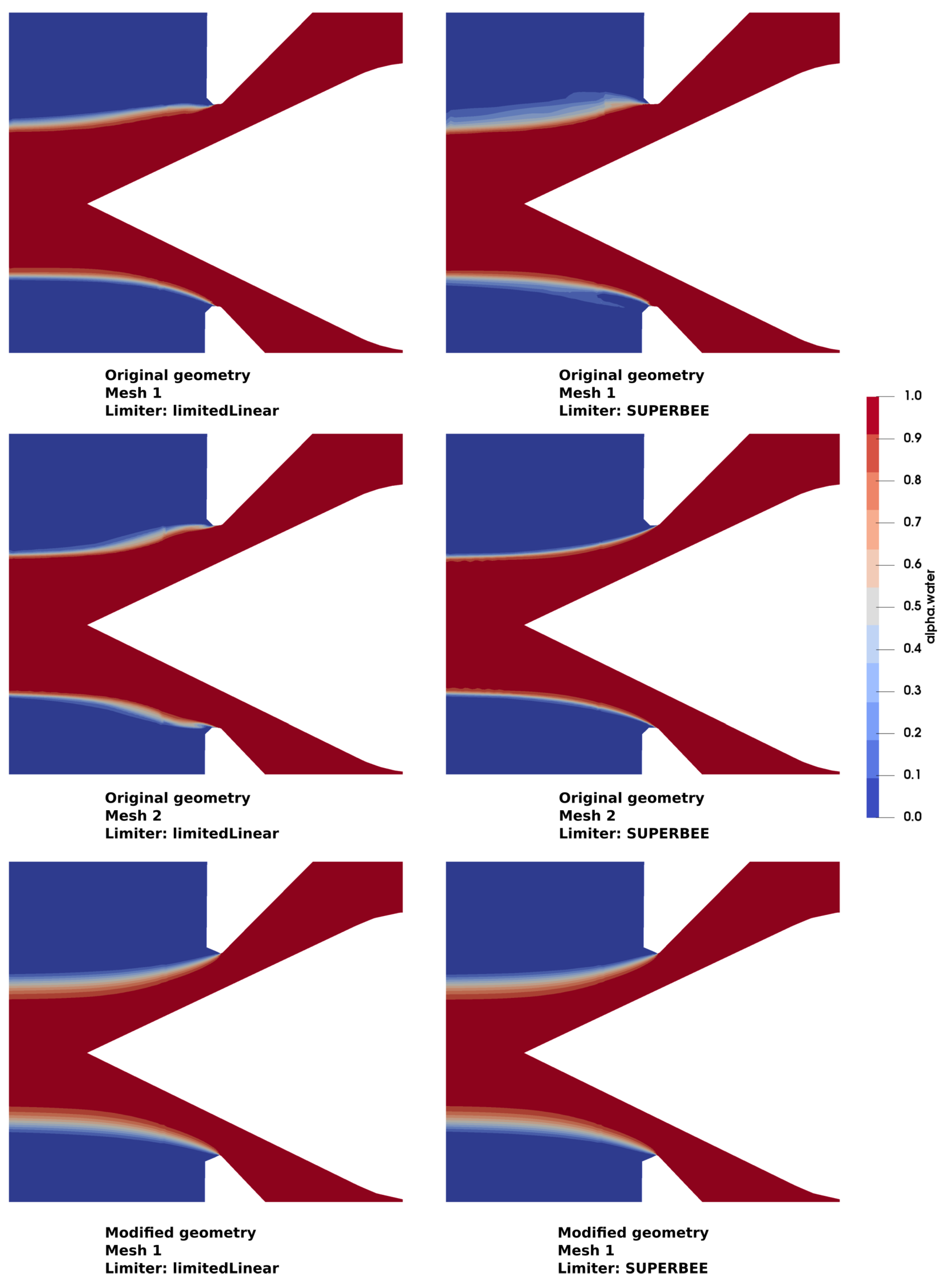
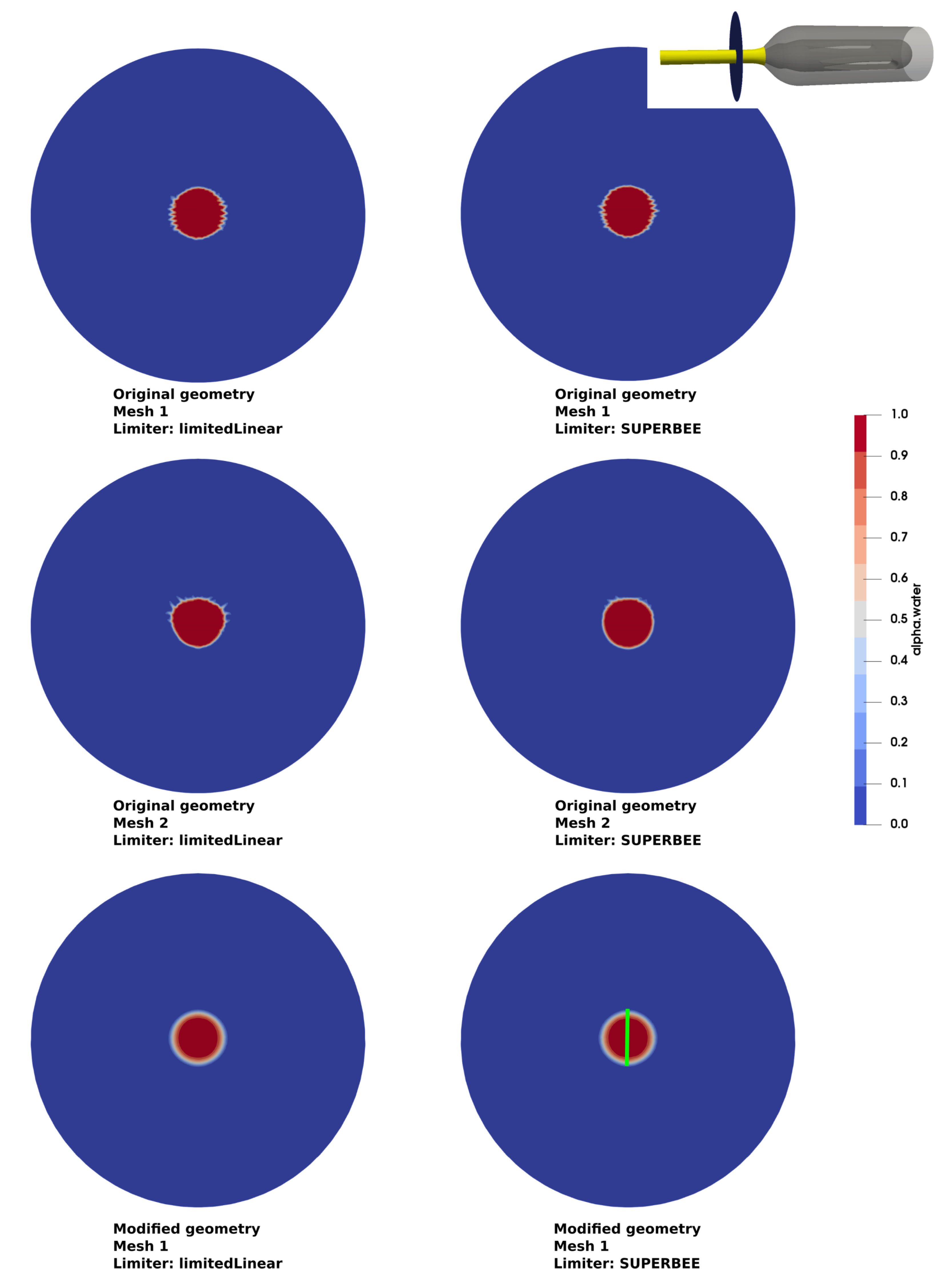
6. Results
7. Conclusions
Author Contributions
Funding
Data Availability Statement
Conflicts of Interest
Abbreviations
| CFD | Compuational Fluid Dynamics |
| FCT | Flux Transport Corrected |
| FMHL+ | Forces Motrices Hongrin-Léman |
| FMV | Forces Motrices Valaisannes |
| KWGO | Kraftwerke Gletsch–Oberwald |
| MULES | Multidimensional Universal Limiter for Explicit Solution |
| RANS | Reynolds-Averaged Navier–Stokes |
| SST | Shear-Stress Transport |
| TVD | Total Variation Diminishing |
References
- Huertas-Hernando, D.; Farahmand, H.; Holttinen, H.; Kiviluoma, J.; Rinne, E.; Söder, L.; Milligan, M.; Ibanez, E.; Martínez, S.M.; Gomez-Lazaro, E.; et al. Hydro power flexibility for power systems with variable renewable energy sources: An IEA Task 25 collaboration. Wiley Interdiscip. Rev. Energy Environ. 2017, 6, 1–20. [Google Scholar] [CrossRef]
- Nechleba, M. Hydraulic Turbines: Their Design and Equipment; Artia: Prague, Czech Republic, 1957. [Google Scholar]
- Widmann, W.; Lebesmühlbacher, T.; Ede, A.; Knorpp, K. Design and operation of the Stanzertal hydro power plant headrace tunnel as reservoir. In Proceedings of the Hydro 2015, Harbor, MD, USA, 16–19 March 2015. [Google Scholar]
- Münch-Alligné, C.; Decaix, J.; Gaspoz, A.; Hasmatuchi, V.; Dreyer, M.; Nicolet, C.; Alimirzazadeh, S.; Zordan, J.; Manso, P.; Crettenand, S. Production flexibility of small run-of-river power plants: KWGO smart-storage case study. IOP Conf. Ser. Earth Environ. Sci. 2021, 774, 012037. [Google Scholar] [CrossRef]
- Micoulet, G.; Jaccard, A.; Rouge, N. FMHL+: Power extension of the existing Hongrin-Léman powerplant: From the first idea to the first kWh. In Proceedings of the Hydro2016, Montreux, Switzerland, 10–12 October 2016. [Google Scholar]
- XFLEX-HYDRO. French Hydropower Plant Aims to Increase Efficiency and Flexibility. XLFEX HYDRO Website. 2022. Available online: https://xflexhydro.net (accessed on 25 May 2022).
- Pérez-Díaz, J.I.; Sarasúa, J.I.; Wilhelmi, J.R. Contribution of a hydraulic short-circuit pumped-storage power plant to the load–frequency regulation of an isolated power system. Int. J. Electr. Power Energy Syst. 2014, 62, 199–211. [Google Scholar] [CrossRef]
- Sick, M.; Keck, H.; Vullioud, G.; Parkinson, E. New Challenges in Pelton Research. In Proceedings of the Hydro 2000 Conference, Engineers, Australia, 20–23 November 2000. [Google Scholar]
- Židonis, A.; Aggidis, G.A. State of the art in numerical modelling of Pelton turbines. Renew. Sustain. Energy Rev. 2015, 45, 135–144. [Google Scholar] [CrossRef]
- Marongiu, J.; Leboeuf, F.; Caro, J.; Parkinson, E. Free surface flows simulations in Pelton turbines using an hybrid SPH-ALE method. J. Hydraul. Res. 2009, 48, 40–49. [Google Scholar] [CrossRef]
- Solemslie, B.W.; Dahlhaug, O.G. A reference Pelton turbine design. Proc. IOP Conf. Ser. Earth Environ. Sci. 2012, 15, 032005. [Google Scholar] [CrossRef]
- Jahanbakhsh, E.; Vessaz, C.; Maertens, A.; Avellan, F. Development of a Finite Volume Particle Method for 3-D fluid flow simulations. Comput. Methods Appl. Mech. Engrg. 2016, 298, 80–107. [Google Scholar] [CrossRef]
- Alimirzazadeh, S.; Kumashiro, T.; Leguizamón, S.; Jahanbakhsh, E.; Maertens, A.; Vessaz, C.; Tani, K.; Avellan, F. GPU-accelerated numerical analysis of jet interference in a six-jet Pelton turbine using Finite Volume Particle Method. Renew. Energy 2020, 148, 234–246. [Google Scholar] [CrossRef]
- Messa, G.V.; Mandelli, S.; Malavasi, S. Hydro-abrasive erosion in Pelton turbine injectors: A numerical study. Renew. Energy 2019, 130, 474–488. [Google Scholar] [CrossRef]
- Tarodiya, R.; Khullar, S.; Levy, A. Assessment of erosive wear performance of Pelton turbine injectors using CFD-DEM simulations. Powder Technol. 2022, 408, 117763. [Google Scholar] [CrossRef]
- Staubli, T.; Abgottspon, A.; Weibel, P.; Bissel, C.; Parkinson, E.; Leduc, J.; Leboeuf, F. Jet quality and Pelton efficiency. In Proceedings of the Hydro 2009, Lyon, France, 26–28 October 2009. [Google Scholar]
- Santolin, A.; Cavazzini, G.; Ardizzon, G.; Pavesi, G. Numerical investigation of the interaction between jet and bucket in a Pelton turbine. Proc. Inst. Mech. Eng. Part A J. Power Energy 2009, 223, 721–728. [Google Scholar] [CrossRef]
- Mack, R.; Moser, W. Numerical Investigation of the Flow in a Pelton Turbine. In Proceedings of the XXIst IAHR Symposium on Hydraulic Machinery and Systems, Lausanne, Switzerland, 9–12 September 2002. [Google Scholar]
- Jost, D.; Meznar, P.; Lipej, A. Numerical prediction of Pelton turbine efficiency. IOP Conf. Ser. Earth Environ. Sci. 2010, 12, 012080. [Google Scholar] [CrossRef]
- Fiereder, R.; Riemann, S.; Schilling, R. Numerical and experimental investigation of the 3D free surface flow in a model Pelton turbine. IOP Conf. Ser. Earth Environ. Sci. 2010, 12, 012072. [Google Scholar] [CrossRef]
- Barth, T.; Jespersen, D. The design and application of upwind schemes on unstructured meshes. In Proceedings of the 27th Aerospace Sciences Meeting. American Institute of Aeronautics and Astronautics, Reno, NV, USA, 9–12 January 1989. [Google Scholar] [CrossRef]
- Brennen, C. Fundamentals of Multiphase Flow; Cambridge University Press: Cambridge, UK, 2012. [Google Scholar]
- Menter, F.R. Review of the shear-stress transport turbulence model experience from an industrial perspective. Int. J. Comput. Fluid Dyn. 2009, 23, 305–316. [Google Scholar] [CrossRef]
- The OpenFOAM Foundation. Available online: https://openfoam.org/ (accessed on 25 May 2021).
- Deshpande, S.S.; Anumolu, L.; Trujillo, M.F. Evaluating the performance of the two-phase flow solver interFoam. Comput. Sci. Discov. 2012, 5, 14016. [Google Scholar] [CrossRef]
- Menter, F.R.; Ferreira, J.; Esch, T. The SST Turbulence Model with Improved Wall Treatment for Heat Transfer Predictions in Gas Turbines. In Proceedings of the International Gas Turbine Congress 2003, Tokyo, Japan, 2–7 November 2003; pp. 1–7. [Google Scholar]
- Zalesak, S.T. Fully Multidimensional Flux-Corrected Transport Algorithms for Fluids. J. Comput. Phys. 1979, 31, 335–362. [Google Scholar] [CrossRef]
- Moukalled, F.; Mangani, L.; Darwish, M. The Finite Volume Method in Computational Fluid Dynamics; Springer: Berlin/Heidelberg, Germany, 2015. [Google Scholar]
- Decaix, J.; Gaspoz, A.; Hasmatuchi, V.; Dreyer, M.; Nicolet, C.; Crettenand, S.; Münch-Alligné, C. Enhanced Operational Flexibility of a Small Run-of-River Hydropower Plant. Water 2021, 13, 1897. [Google Scholar] [CrossRef]


| Mesh | Geometry | Stroke (%) | Number of Points | Number of Cells | Number of Wall Cell Layers |
|---|---|---|---|---|---|
| 1 | Original | 50 | 5.8 × 10⁶ | 5.1 × 10⁶ | 3 |
| 2 | Original | 50 | 10.1 × 10⁶ | 9.3 × 10⁶ | 3 |
| 1 | Modified | 50 | 5.8 × 10⁶ | 5.1 × 10⁶ | 3 |
| 1 | Original | 85 | 6.3 × 10⁶ | 5.5 × 10⁶ | 3 |
| Mesh | Geometry | Stroke (%) | Maximum Non-Orthogonality (deg) | Maximum Skewness | Maximum Aspect Ratio |
|---|---|---|---|---|---|
| 1 | Original | 50 | 69 | 4.9 | 25 |
| 2 | Original | 50 | 70 | 4.9 | 25 |
| 1 | Modified | 50 | 69 | 6.7 | 26 |
| 1 | Original | 85 | 70 | 4.9 | 25 |
| Mesh | Geometry | Stroke (%) | (−) “limitedLinear” | (−) “SUPERBEE” | (%) |
|---|---|---|---|---|---|
| 1 | Original | 50 | 1.0475 | 1.03 | 1.7 |
| 2 | Original | 50 | 1.0175 | 0.995 | 2.3 |
| 1 | Modified | 50 | 0.965 | 0.965 | 0.0 |
| 1 | Original | 85 | 1.4275 | 1.4075 | 1.4 |
| Mesh Number | Geometry | Stroke (%) | (−) Computed | (−) Exp | (%) |
|---|---|---|---|---|---|
| 1 | Original | 50 | 1.03 | 3.0 | |
| 2 | Original | 50 | 0.995 | 1 | −0.5 |
| 1 | Modified | 50 | 0.965 | −3.5 | |
| 1 | Original | 85 | 1.4075 | 1.3675 | 2.9 |
Publisher’s Note: MDPI stays neutral with regard to jurisdictional claims in published maps and institutional affiliations. |
© 2022 by the authors. Licensee MDPI, Basel, Switzerland. This article is an open access article distributed under the terms and conditions of the Creative Commons Attribution (CC BY) license (https://creativecommons.org/licenses/by/4.0/).
Share and Cite
Decaix, J.; Münch-Alligné, C. Geometry, Mesh and Numerical Scheme Influencing the Simulation of a Pelton Jet with the OpenFOAM Toolbox. Energies 2022, 15, 7451. https://doi.org/10.3390/en15197451
Decaix J, Münch-Alligné C. Geometry, Mesh and Numerical Scheme Influencing the Simulation of a Pelton Jet with the OpenFOAM Toolbox. Energies. 2022; 15(19):7451. https://doi.org/10.3390/en15197451
Chicago/Turabian StyleDecaix, Jean, and Cécile Münch-Alligné. 2022. "Geometry, Mesh and Numerical Scheme Influencing the Simulation of a Pelton Jet with the OpenFOAM Toolbox" Energies 15, no. 19: 7451. https://doi.org/10.3390/en15197451
APA StyleDecaix, J., & Münch-Alligné, C. (2022). Geometry, Mesh and Numerical Scheme Influencing the Simulation of a Pelton Jet with the OpenFOAM Toolbox. Energies, 15(19), 7451. https://doi.org/10.3390/en15197451