Optimal Rotating Receiver Angles Estimation for Multicoil Dynamic Wireless Power Transfer

Abstract

This study proposed an approach to dynamic wireless charging that uses a rotating receiver coil. Our simulation study focused on the verification of a novel way of increasing the coupling coefficient and power transfer stability by following the flux of the transmitting coils. To obtain the highest possible coupling by means of the FEM analysis, we studied the optimization of the trajectory of the angular velocity of the rotating receiver. The coupling coefficient trajectories that were obtained were simulated by means of the state space model with three transmitters. Our comprehensive analysis showed that the proposed approach of wireless power transmission enabled a 40% increase in the usage of track space.

1. Introduction

The number of wireless car chargers has started to increase. The idea of continuous and unobstructed charging while the electric vehicle (EV) is moving has emerged to improve the comfort and convenience of using the vehicle. Such technology is called dynamic wireless power transfer (DWPT). Despite certain difficulties and limitations, the technology is promising and is already being actively implemented [1,2,3].

The conventional DWPT system that is used for car charging is generally constructed using flat transmission coils that are built into the road’s surface and the receiving coil(s) are attached to the bottom of the vehicle. The system can be composed of a centralized or segmented structure (Figure 1) [4].

In the centralized power supply structure (Figure 1a), a large transmitting coil is installed on the road’s surface. The centralized scheme has higher losses, high installation, and higher maintenance costs than the segmented scheme [4]. In comparison with the receiver coil (Rx), larger sizes of the transmitter (Tx) coils cause a low coupling coefficient rating, leading to decreased efficiencies [3]. Segment-based solutions are more efficient because segments can be individually controlled [3]. The system structure has an array of transmission coils (Figure 1b). One example of such a project is the Versailles–Satory Site [5]—EV with a charging capacity of up to 20 kW.

Table 1. Comparison of non-uniformity of energy transmission for a DWPT.

System and Reference	Efficiency Variation during Movement	Power Variation during Movement	Coupling Variation during Movement
[5]	85–97% (12%)	Up to 50% (10–20 kW)	-
[6]	0–57% (57%)	100% (0–30 W)	0.05–0.9 (0.85 difference)
[6]	-	7–30 W	0.1–0.95
[7]	10–30%	-	0–0.2
[7]	45–76%	-	0–0.2
[8]	-	5.2–32 W	0.1–0.45
[9]	88–97%	600–1500 W	0–0.2

clarifies the limitations of uneven energy transfer and compares its magnitude in different situations, mainly in the segmented structure of a DWPT. The decrease in the transmission power can be more than 50% of the maximum value (up to the absence of the received energy at certain intervals).

Most of these works focused on various shapes of magnetic coils and cores [10,11,12,13,14,15]. At the same time, the main disadvantage lay in the non-uniformity of the charging current (uneven transmission/reception of energy) during movement. In certain positions, the receiving coil is not exactly above the transmitting coils, resulting in a limited amount of efficiently transferred energy. The aim of this study was to propose, analyze and verify an approach to dynamic wireless charging with an array of flat transmitting coils and a rotating receiver, which improved the uniformity of the energy transfer.

Rotating coil systems are widely used in industry [16,17,18,19,20,21,22,23]. For example, in [23], a novel approach of transmission efficiency valley of death (TEVD) was proposed for the magnetic-resonance-coupled WPT system to reduce lateral misalignments. In this system, the receiving flat spiral coil rotates at a certain angle depending on the distance to the receiving coil so that the magnetic flux always passes the receiver in one direction and is as large as possible through the area of the coil (Figure 2). This increases the efficiency and the operating range of distances. However, [23] showed only one transmitting and receiving coil and the authors used it as a system of static charging with a locking receiving coil at certain distances.

In the dynamic charging of vehicles (linear movement), no solutions with a rotating receiving coil at the optimal angle have been reported. The purpose of our solution was to provide stable (uniform) energy transfer and efficiency while driving a vehicle at different speeds with a DWPT for a segmented structure with flat coils.

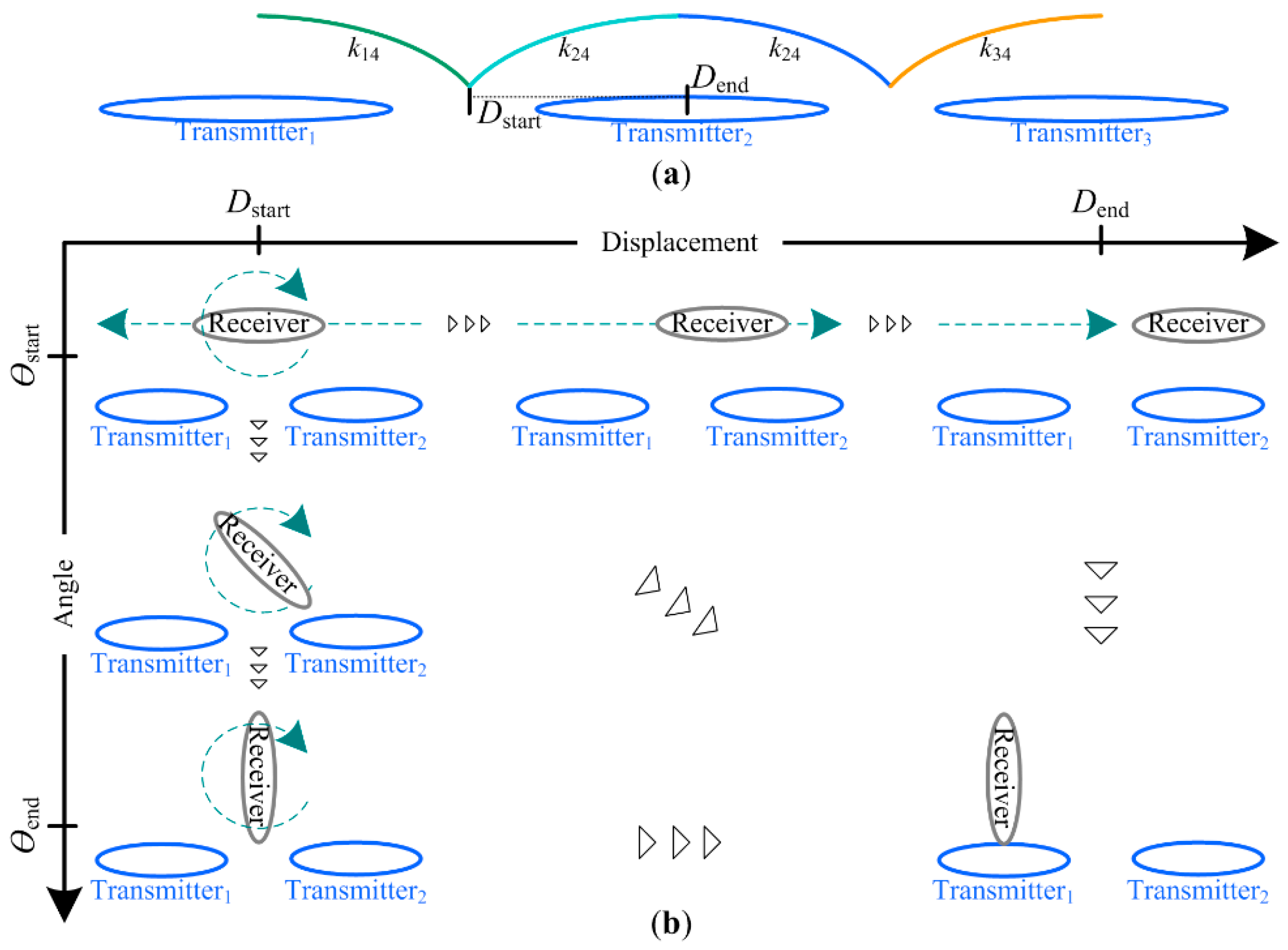
2. Moving Track Model Study

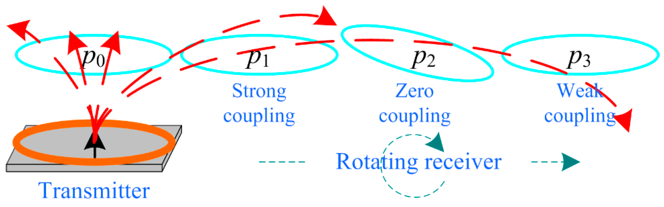
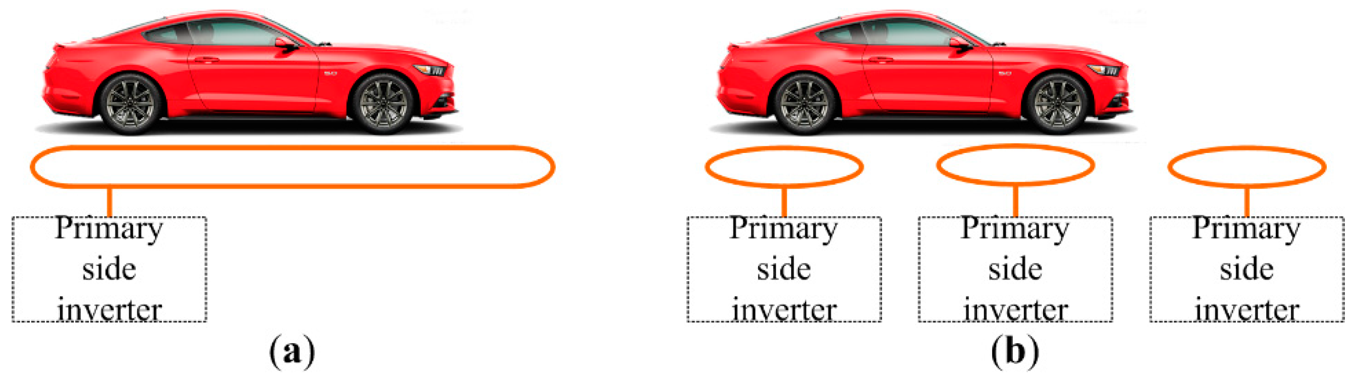
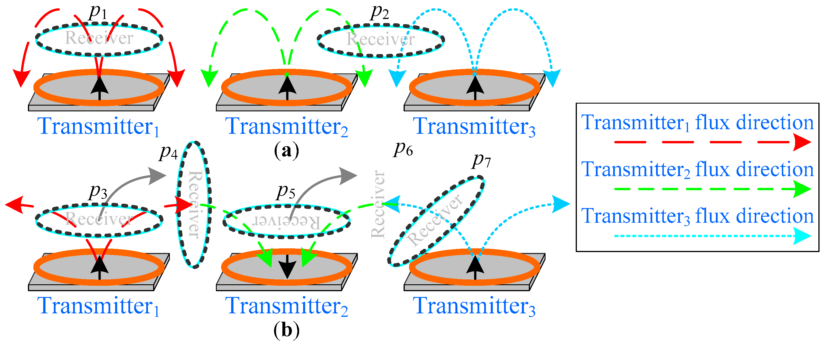
2.1. Description of the Approach

The conventional segmented track solution is shown in Figure 3a. This solution gives high performance for aligned coils (position p₁), but in other cases during movement and especially in positions when the receiver is situated between two transmitters (position p₂), only a small part of the flux is passing through the coil. Additionally, depending on the coil design for a displacement that is approximately equal to coil radius (depends on coil design), the amount of transmitted flux that passes through the receiver has the same magnitude but opposite direction and they cancel each other. There is no possibility to reduce this influence without decreasing the distance between the transmitters and correspondingly increasing the amount of transmitting coils on the same distance of the track.

Unlike the conventional solution, the proposed method (Figure 3b) does not suffer from such problems as in an approach where the receiver coil is rotating according to the flux of the transmitters. By turning on the nearby transmitting coils in the opposite direction, it is possible to attain a system where the transmitter flux will always pass through the receiver coil in one direction. However, this leads to the case with no positions where the transmitter flux passes the receiver coil in the opposite direction and more flux can pass the receiver coil. In this case, a coupling coefficient that is higher than that in the conventional solution is expected when using non-aligned positions (positions p₄ and p₆).

The proposed coil system was connected to the inverter (Figure 4). The topology consisted of 12 switching elements (Figure 4), which was sufficient to implement three coil power transmitters. To obtain high power transfer efficiency and to omit circulating reactive currents that decrease the system’s efficiency and reliability, the compensation capacitors were connected in series with transmitting and receiving coils. It is also possible to connect these capacitors in parallel, but in such cases, it is necessary to make additional system tuning. For example, for cases of SP type of compensation, the reflected impedance involves coupling the dependent reactance part, which makes it unreliable to use such an approach in dynamic charging.

As the system works in a resonant mode, the topology can be represented using a simplified model, as shown below (Figure 5). This model was sufficient to enable precise estimation of the main relations between the transmitters and the receiver of the proposed solution. As can be seen, the inverter was replaced by a voltage input v_in1. The full-bridge rectifier, filter and load could be represented using an equivalent resistor, which consumed the same amount of power as the solution with a full bridge [24]. Such a load could be estimated using (1). The model involved losses in the transmitter (R_l1, R_l1, R_l1) and receiver coils (R_l4).

R_Leq = (8/π²)(V²_2,dc/P₂)

(1)

Coupled coils were represented using a model with mutual inductance. In comparison to the solution with self and leakage inductances, this model could simplify the system order. There were six mutual inductances. M₁₄, M₂₄ and M₃₄ represent coupling between the transmitters and the receiver, while M₁₂, M₂₃ and M₁₃ represent coupling between the transmitters and, in some cases, the large distance between the transmitters could be neglected.

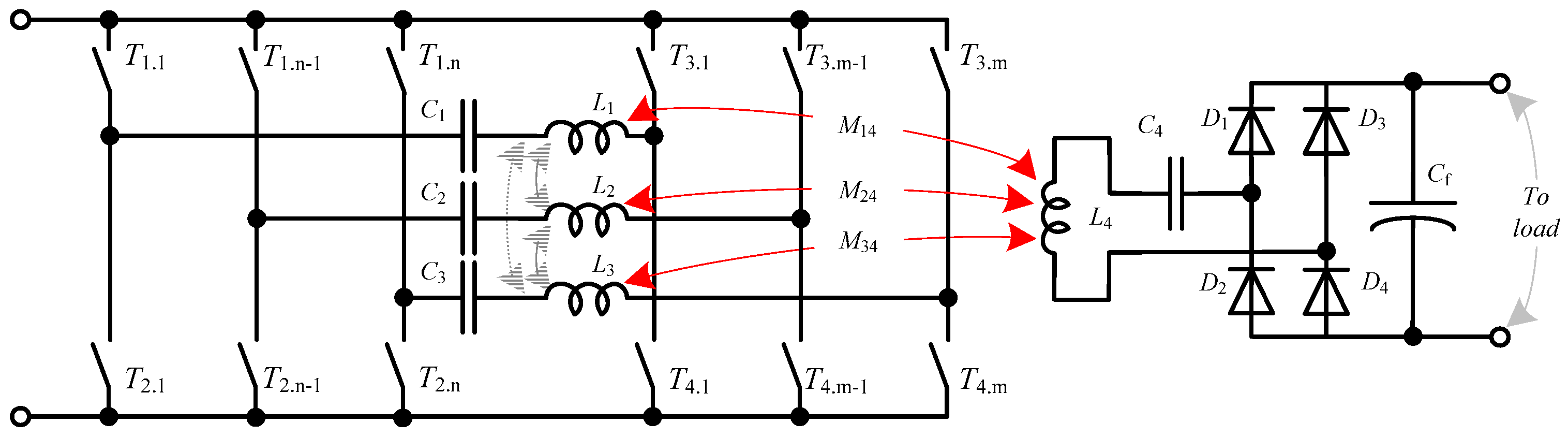
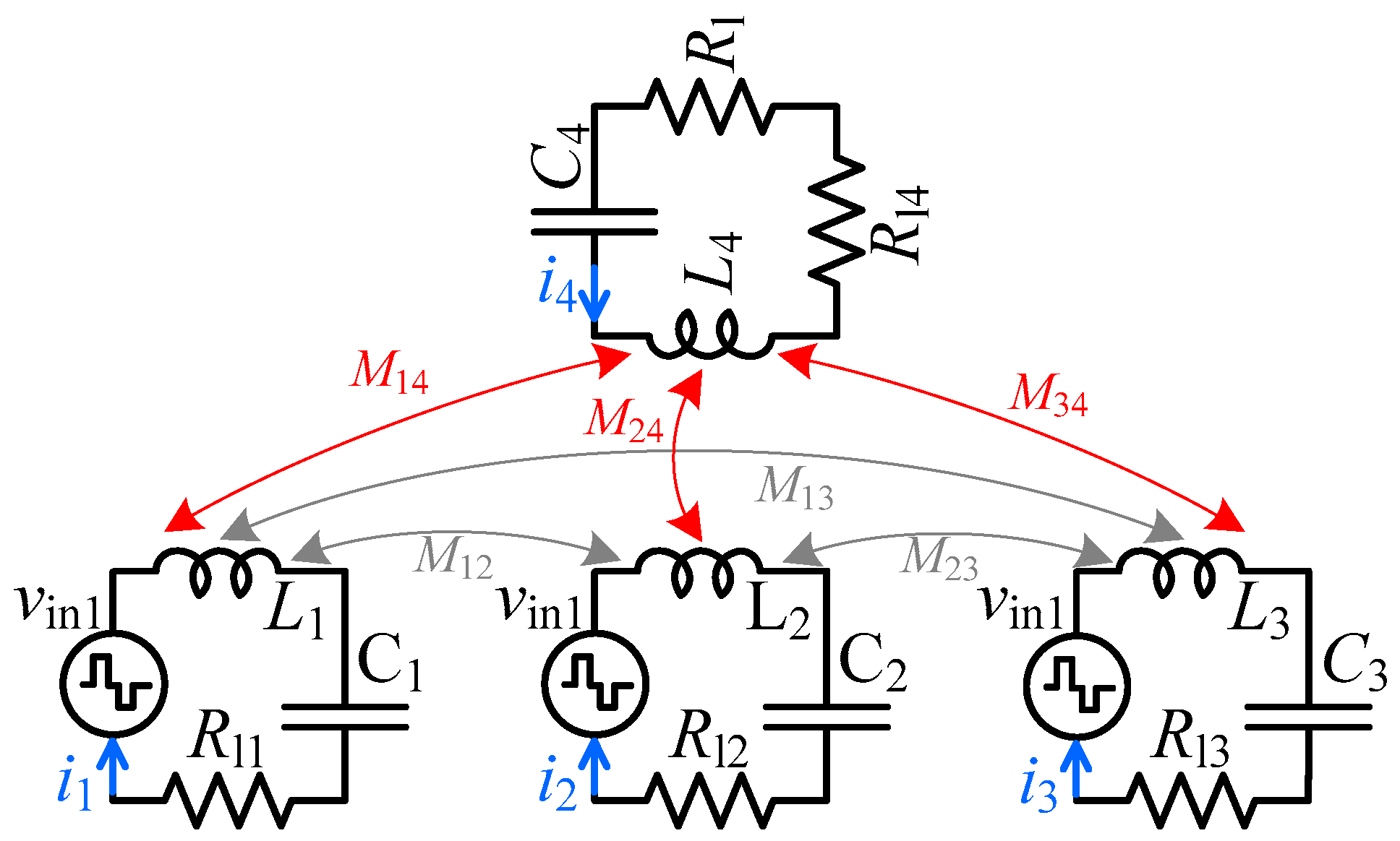
2.2. State Space Model of the Power Transmitter Link

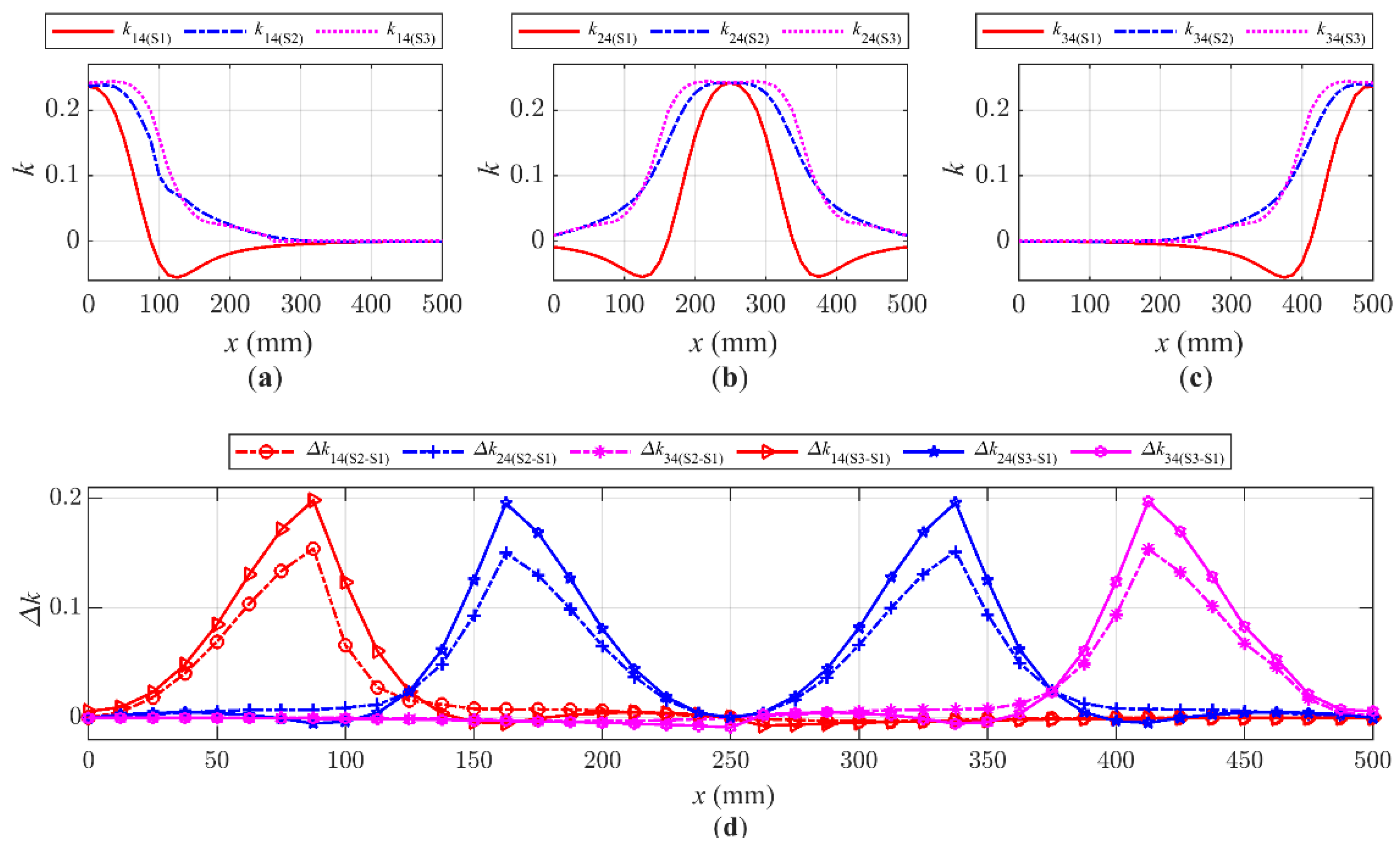
Based on the simplified topology model, a wireless transmitting system could be represented using an eighth-order system of differential Equation (2).

$$\{\begin{array}{c}{v}_{in1}=v_{\mathrm{c}1}(t)+L_1(t)\frac{d{i}_1(t)}{dt}-M_{12}(t)\frac{d{i}_2(t)}{dt}-M_{13}(t)\frac{d{i}_3(t)}{dt}-M_{14}(t)\frac{d{i}_4(t)}{dt}+i_1(t)\cdot R_{l1}\\ v_{in1}=v_{\mathrm{c}2}(t)+L_2(t)\frac{d{i}_2(t)}{dt}-M_{12}(t)\frac{d{i}_1(t)}{dt}-M_{23}(t)\frac{d{i}_3(t)}{dt}-M_{24}(t)\frac{d{i}_4(t)}{dt}+i_2(t)\cdot R_{l2}\\ v_{in1}=v_{\mathrm{c}3}(t)+L_3(t)\frac{d{i}_3(t)}{dt}-M_{13}(t)\frac{d{i}_1(t)}{dt}-M_{23}(t)\frac{d{i}_2(t)}{dt}-M_{34}(t)\frac{d{i}_4(t)}{dt}+i_3(t)\cdot R_{l3}\\ 0=v_{\mathrm{c}4}(t)+L_4(t)\frac{d{i}_4(t)}{dt}-M_{14}(t)\frac{d{i}_1(t)}{dt}-M_{24}(t)\frac{d{i}_2(t)}{dt}-M_{34}(t)\frac{d{i}_3(t)}{dt}+i_4(t)\cdot R_{l4}+i_4(t)\cdot R_l\\ i_1(t)=C_1\frac{d{v}_{\mathrm{c}1}(t)}{dt}\\ i_2(t)=C_2\frac{d{v}_{\mathrm{c}2}(t)}{dt}\\ i_3(t)=C_3\frac{d{v}_{\mathrm{c}3}(t)}{dt}\\ i_4(t)=C_4\frac{d{v}_{\mathrm{c}4}(t)}{dt}\end{array}$$

(2)

To use the model in a dynamic charging simulation, this system of differential equations could be rewritten as a time-domain-continuous time-variant SIMO state-space model (3). The values of the state matrix A(t) and the input matrix B(t) varied according to the coupling coefficients in the corresponding receiver position. The input vector u(t) consisted of one element, namely, v_in1.

The state vector in the proposed model was represented by eight elements. The vector consisted of four currents in the coils (i₁, i₂, i₃ and i₄) and four voltages across the compensation capacitors (v_c1, v_c2, v_c3 and v_c4), which were represented as [i₁ i₂ i₃ i₄ v_c1 v_c2 v_c3 v_c4]^T.

$${\left[\begin{array}{cccccccc}\stackrel{•}{i_1}& \stackrel{•}{i_2}& \stackrel{•}{i_3}& \stackrel{•}{i_4}& \stackrel{•}{v_{\mathrm{c}1}}& \stackrel{•}{v_{\mathrm{c}2}}& \stackrel{•}{v_{\mathrm{c}3}}& \stackrel{•}{v_{\mathrm{c}4}}\end{array}\right]}^T=A(t)\cdot {\left[\begin{array}{cccccccc}\stackrel{}{i_1}& i_2& i_3& i_4& v_{\mathrm{c}1}& v_{\mathrm{c}2}& v_{\mathrm{c}3}& v_{\mathrm{c}4}\end{array}\right]}^T+B(t)\cdot \left[v_{in1}\right]$$

(3)

The output matrix was chosen as the identity matrix to obtain output vector values that were identical to all elements of the state vector.

3. Simulation Study

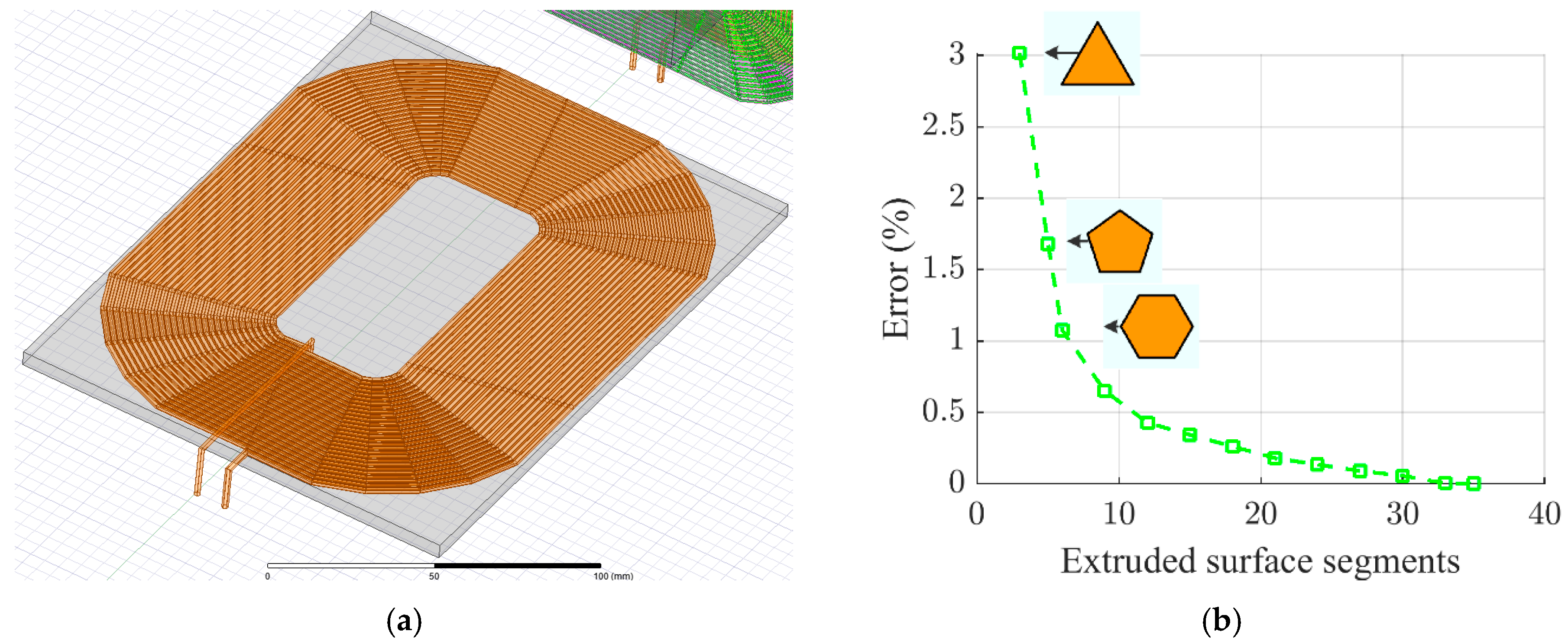
3.1. Simulation Model Description

The simulation study was divided into two stages. For each solution, in the first stage, the finite element analysis (FEA) was performed to obtain the trajectories of coupling coefficient variations for different receiver displacements and angles.

In the second stage, with the obtained trajectories, the simulation of the power transfer process dynamics was made by solving the state-space equations shown before. For this purpose, the Runge–Kutta fourth-order method was used to solve the differential equations. This method has sufficient accuracy along with a decreased simulation time. All the calculations were performed in the Matlab numeric computing environment and its programming language. As the system operated at a high frequency and under resonance to obtain precise and sufficient calculations, the differential equations were solved with a 1 × 10⁻⁹ s time step.

To estimate the coupling coefficients between the transmitting and the receiving coils, a 3D FEM simulation was performed in ANSYS MAXWELL software. The receiver and transmitter coils were generated using a developed script in the Python language, which extruded the hexagonal shape of the cross-section along the proposed coil shape. As shown in the simulation analysis (Figure 6b), the hexagonal shape was sufficient for precise measurements with an accuracy of ~1%. An increased amount of extruded surface segments increased the accuracy by only a limited amount, but the computational requirements were significantly increased. The estimated coil inductances are given in

Table 2. FEM and electrical model parameters.

Description	Symbol	Value	Unit
Track length	-	500	mm
Primary side coil turns	N1	28	-
Secondary side coil turns	N2	17	-
Primary side coil wire diameter	d1	2	mm
Secondary side coil wire diameter	d2	2	mm
Primary side coil dimensions	-	150 × 200	mm
Secondary side coil dimensions	-	98 × 144	mm
Input voltage	vin1	315	V
Switching frequency	fsw	100	kHz
Primary side inductances	L1, L2, L3	191.26 ± 0.67%	μH
Secondary inductance	L4	61.63 ± 4.92%	μH
Primary side capacitance	C1, C2, C3	13.24	nF
Secondary side capacitance	C4	41.1	nF
Coil resistances	Rl1, Rl2, Rl3, Rl4	0.5	Ω
Output load	Rl	10	Ω

. There was a deviation in the self-inductance during movement, which was caused by the influence of the ferrite shields. According to the simulation results, the parameter deviation was less than 5% and, therefore, was neglected in the analysis.

The designed transmitter coils are shown in Figure 6a. The oval shape of the transmission coils was chosen to extend the coils in the longitudinal direction of movement in order to increase the effective transmission area. To increase the coupling coefficient, ferrite shielding for the transmitters with a relative permeability of 1000 was used. The size of the ferrite core was made large enough to ensure reliable conduction of the flow in any position. The thickness of the ferrite shielding was chosen by taking into consideration the material dimensions of available products.

The resulting system was simulated using relevant parameters of the air environment, with the size of the simulated environment being 770 × 180 × 130 mm.

The design of the receiver coil with ferrite material to concentrate the flux is shown in Figure 6c. The design of the coil was chosen to obtain the lowest distance between the receiver and the transmitter coils and to overcome the intersection of the system elements in all positions during the receiver’s movement.

First, to verify the model and to calculate the system parameters, the simulation was undertaken in the static mode for separately activated transmitters. For simplicity, only one input source (v_in1) was used in the model. In that case, separate coils could be deactivated by increasing the coil resistance values R_l1, R_l2 and R_l3. Increasing the coil resistances (R_l(_1,2,3)→∞) corresponded to very small changes in the current passing through the corresponding part of a circuit (i_(1,2,3)→0). The simulation showed that such an approach worked and that only one sinusoidal current of valuable magnitude appeared in the transmitter coils (Figure 7c–e). Figure 7f–h demonstrate that the receiver current remained sinusoidal for each transmitter activation.

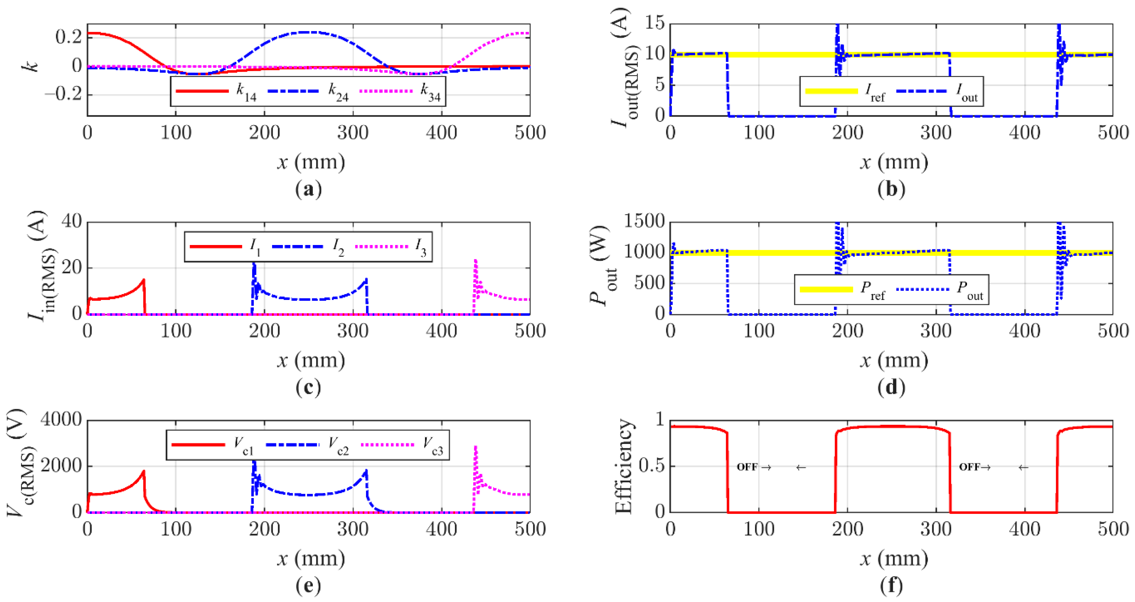
3.2. Simulation of a Dynamically Moving Receiver

For an accurate comparison between the conventional solution and the proposed solution with a rotating receiver, the simulation study focused on the constant current (CC) output mode and constant output power. For this purpose, a PID controller was used. To obtain the RMS value of the output current that was used as feedback in the PID controller error estimation, the RMS values of the last 5000 samples of the output current i₄ were taken. The reference current was set to 10 A and with the equivalent resistor R_l = 10 Ω, the output power P_out was 1 kW.

To clarify the advantages of the proposed solution and to make a comparison under the same operating conditions, all simulations were performed for a situation in which only one transmitter was being activated. Additionally, the activation of a particular coil was made for a fixed coupling coefficient for all the performed simulations.

The simulation results of the conventional solution are presented in Figure 8. As was expected, during the displacement of the flux, which was passing through the receiver coil, its direction (~90 mm) was changing (Figure 8a) and, in some positions, it was opposite to the flux of the next transmitting coil (~70.90 mm). In that case, to expand the area of charging and use two transmitters simultaneously, it was necessary to change the flux direction of the transmitters to omit situations when two transmitter fluxes were canceling each other and no power was being transmitted to the receiver.

As the proposed simulations did not involve changes in the flux direction with the defined coupling coefficient, only ~52% of the track distance was used during charging (Figure 8d). To increase the usage of the track, the activation coupling coefficient could be decreased, but this would lead to a very large reduction in efficiency and reliability. Additionally, the maximum efficiency was obtained for only one value of displacement for each transmitting coil (Figure 8f).

As can be seen from Figure 9, in the proposed solution, the track area with a higher coupling coefficient rapidly expanded (Figure 9a). This corresponded to the increased track area where power transmission under high coupling and a correspondingly high efficiency could be achieved.

It should also be mentioned that there were no positions where the flux changed its direction (Figure 9a); therefore, there was no necessity to change the flux direction to expand the track’s area of transmission.

The coupling coefficient (Figure 9a) also revealed that the point of the highest efficiency was expanded to the high range of the receiver displacement variation. Thus, in such a solution, the valuable part of the transmitted energy was being transmitted with a maximum coupling coefficient and with the highest stability (in this region, the CC mode PID controller worked for a nearly constant coupling coefficient).

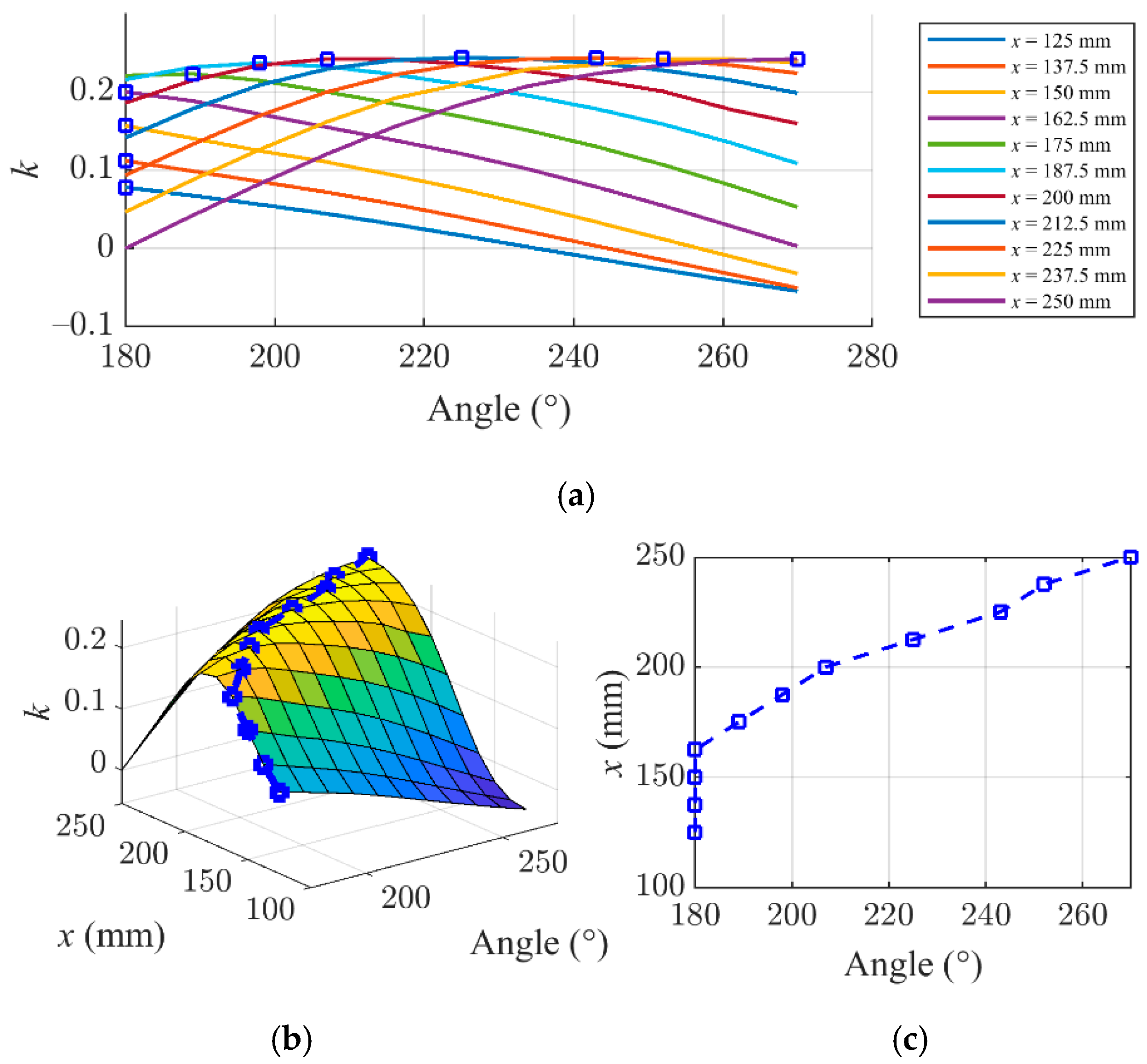
4. Optimal Movement Trajectory Study

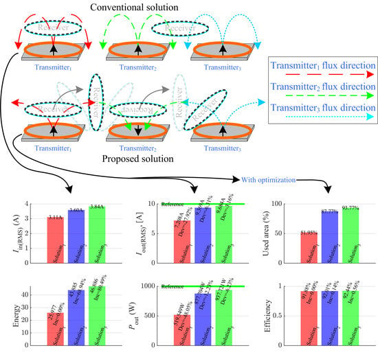
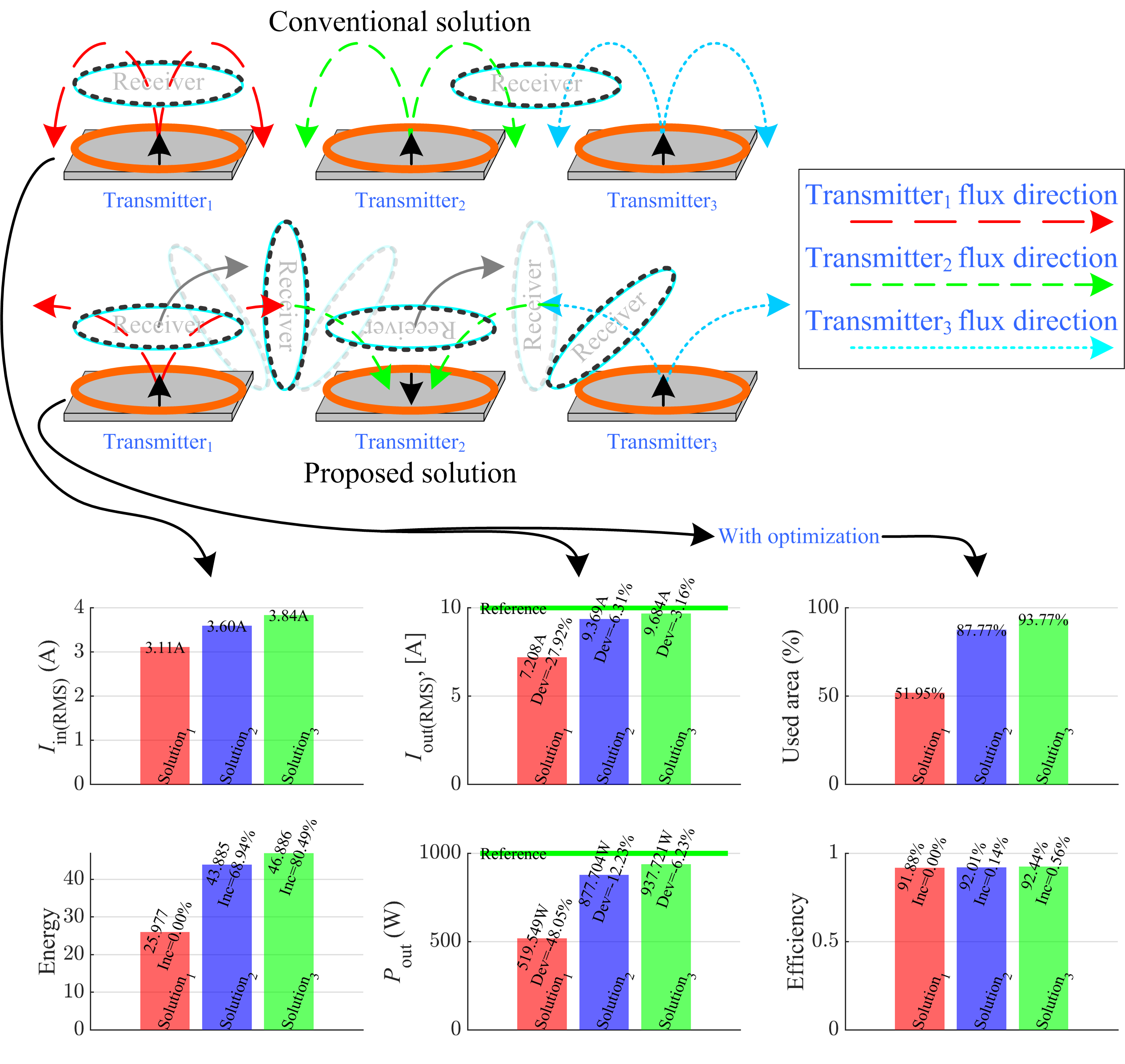
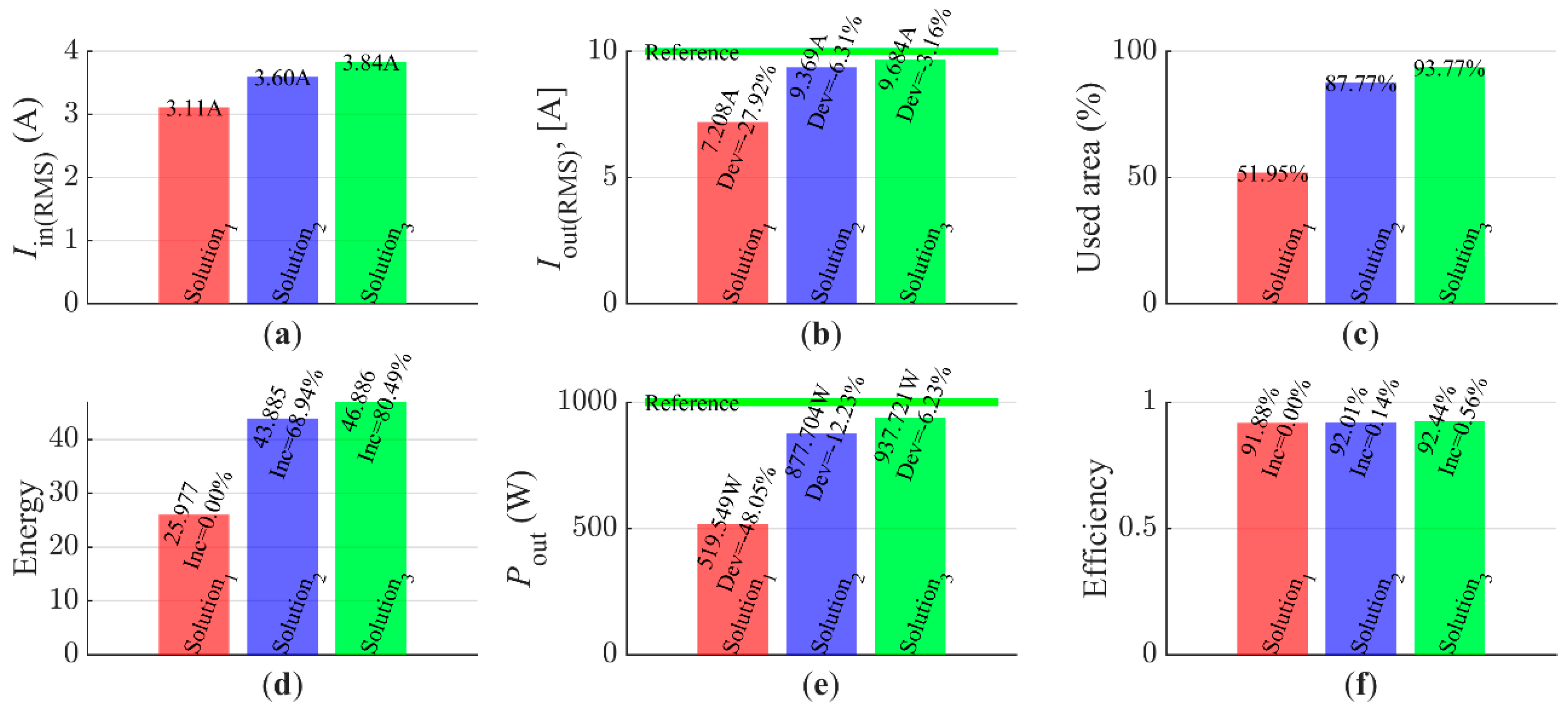
The simulation results showed that the proposed solution with a rotating receiver could increase both system efficiency and the amount of transmitted power. Conversely, by taking into account the fact that the nonlinearity of ferrite materials complicates the estimation of the flux direction in each position, it was possible to find the optimal angle where a greater flux from the transmitters was penetrating the receiver coil for each position during movement. As was shown in the previous simulations, in the case of the multicoil solutions, the trajectory of the coupling coefficient variation was repeated in each section (Figure 10a). This provided the ability to find optimal angles for small parts of the track (in the range D_start–D_stop) and then by mirroring and merging trajectories to obtain the optimal movement along the whole track.

The ranges of the receiver coil angle and position variations with the corresponding simulation steps are listed in

Table 3. Simulation parameters for the FEM optimization.

Description	Symbol	Value	Unit
Start angle	θstart	180	°
Angle step	θstep	9.0	°
End angle	θend	270	°
Start position	Dstart	125	mm
Position step	Dstep	12.5	mm
End position	Dend	250	mm

.

Figure 11a gives the simulation results. It can be seen that the maximum efficiency along the track remained the same and that the angle of the receiver coil had a strong influence on the value of the coupling coefficient.

To obtain a better understanding of the proposed solution, the results of the simulations were represented as a surface (Figure 11b) depending on the displacement D and the angle of rotation θ. By finding the maximum possible value of the coefficient for each position, the trajectory of movement was estimated.

The projection of the trajectory on a displacement–rotation plane is shown in Figure 11c. For this coil design, the track part between the coils (125–162.5 mm) should remain at the same vertical angle (180°) to obtain the highest possible coupling coefficient.

The simulation results for the optimized receiver coil rotation (Figure 12) showed that the conditions of the one-way flux of the rotating receiver remained the same (Figure 12a). Additionally, the coupling coefficients along the entire track increased, which created the opportunity to activate the transmitting coils earlier. This increased the amount of transmitted energy due to the higher efficiency (Figure 12d) in comparison to the solution with a constant angular velocity (Figure 9d).

Taking into account the additional complexity of the implementation, which is related to searching for the optimal trajectory of rotation, this solution can be used for systems where stability of the transmitted power is more critical. In other cases, the solution with constant angular velocity is more suitable, as there is no necessity to follow the nonlinear trajectory of movement.

5. Comparison

The coupling coefficients for different solutions under different receiver positions are shown in Figure 13a–c. The expanded area of the proposed solution along with the lack of flux direction changes can be clearly seen.

To compare the conventional solution with the proposed solution, the differences in couplings were calculated. The results are shown in Figure 13d. There were positions where the difference in the coupling coefficient nearly reached the maximum coupling coefficient value. In this position, the first solution had a zero coupling coefficient, which, as was said earlier, corresponded to positions where the inner and outer fluxes canceled each other.

To compare all three solutions, the averaged values of the main parameters were calculated over the entire simulation range. The output current and the output power are shown in Figure 14b,e. Although during power transmission, the system kept the same output current and power, it can be seen that the RMS value along the whole track deviated significantly from the reference parameter in the first solution. The reason was that the first solution was based on high ranges along the track with a low coupling coefficient such that the power was being transmitted over a smaller range.

To estimate the differences in the amount of the transmitted power, the output power was integrated over time along all simulation ranges to obtain the output energy. Figure 14d shows that the second and third solutions enabled the transmission of more energy with the same receiver configuration. Additionally, with the increased coupling coefficient, the area of transmission was increased. In the third solution, 93% of the area was used for transmitting (Figure 14c), which was nearly twice as large as in the conventional solution.

6. Conclusions

The simulation results confirmed that among the three options (cases) for placing the receiving coil, the optimal method (solution) was rotation with optimal angles of rotation.

The proposed solution has many advantages. For transmitting coils with opposite flux directions, the flux of nearby coils was pointed in one direction and there were no points at which the transmitter fluxes canceled each other. This means that there was no necessity to switch the flux direction of the transmitting coils and, correspondingly, a simplified inverter topology could be used. By involving the rotation of the receiver along with movement and by following the flux direction, the transmitted energy could be harvested more effectively. This corresponded to higher coupling between the receiver and the transmitters. As the coupling coefficients between the receiver and the transmitter were higher over a wider range of displacements, it enabled a power transfer over a wider range and, as a result, a more stable energy transfer could be obtained during the receiver movement.

As the second and third solutions involved moving along the track with a predefined movement trajectory and with a higher coupling coefficient, with the valuable part of the energy being transmitted at the highest possible coefficient, these solutions gave a 0.17 and a 0.66 increase in the system efficiency (Figure 14f). For the solutions where the highest possible efficiency was not necessary, the second solution can be used as a trade-off between low efficiency and increased system complexity (solution 3).

This solution can be applied in different ways, primarily in dynamic charging systems where the distance between the road (rails) to the coil (the bottom of the vehicle) does not change. Another excellent option is in rail transport where the air gap is constant. The solution proposed in this article can also be used for a centralized DWPT system, but it would be more expedient and relevant for the segmented option due to the larger number of transmission coils. The task for the future is to study the different geometric shapes of coils and ferrite cores and to collect data on the induction flux during rotation to be able to obtain greater energy transfer efficiency. It will also be important to develop and implement intelligent onboard real-time algorithms for the control of the receiving coil and the adjustment of the angular speed of rotation of the receiving coil depending on the linear speed of the vehicle. Another important future area of study will be the experimental verification of the presented solution.

References

1. Shevchenko, V.; Husev, O.; Strzelecki, R.; Pakhaliuk, B.; Poliakov, N.; Strzelecka, N. Compensation Topologies in IPT Systems: Standards, Requirements, Classification, Analysis, Comparison and Application. IEEE Access 2019, 7, 120559–120580. [Google Scholar]
2. Patil, D.; McDonough, M.K.; Miller, J.M.; Fahimi, B.; Balsara, P.T. Wireless Power Transfer for Vehicular Applications: Overview and Challenges. IEEE Trans. Transp. Electrification 2017, 4, 3–37. [Google Scholar] [CrossRef]
3. Jayathurathnage, P.K.S.; Alphones, A.; Vilathgamuwa, D.M.; Ong, A. Optimum Transmitter Current Distribution for Dynamic Wireless Power Transfer with Segmented Array. IEEE Trans. Microw. Theory Tech. 2017, 66, 346–356. [Google Scholar] [CrossRef]
4. Panchal, C.; Stegen, S.; Lu, J.-W. Review of static and dynamic wireless electric vehicle charging system. Eng. Sci. Technol. Int. J. 2018, 21, 922–937. [Google Scholar] [CrossRef]
5. Laporte, S.; Coquery, G.; Deniau, V.; De Bernardinis, A.; Hautière, N.; Bernardinis, D. Dynamic Wireless Power Transfer Charging Infrastructure for Future EVs: From Experimental Track to Real Circulated Roads Demonstrations. World Electr. Veh. J. 2019, 10, 84. [Google Scholar] [CrossRef] [Green Version]
6. Anyapo, C.; Teerakawanich, N.; Mitsantisuk, C.; Ohishi, K. Experimental Verification of Coupling Effect and Power Transfer Capability of Dynamic Wireless Power Transfer. In Proceedings of the 2018 International Power Electronics Conference (IPEC-Niigata 2018—ECCE Asia), Niigata, Japan, 20–24 May 2018; pp. 3332–3337. [Google Scholar]
7. Sampath, J.P.K.; Vilathgamuwa, D.M.; Alphones, A. Efficiency Enhancement for Dynamic Wireless Power Transfer System with Segmented Transmitter Array. IEEE Trans. Transp. Electrif. 2015, 2, 76–85. [Google Scholar] [CrossRef]
8. Anyapo, C. Development of Long Rail Dynamic Wireless Power Transfer for Battery-Free Mobile Robot. In Proceedings of the 2019 10th International Conference on Power Electronics and ECCE Asia (ICPE 2019-ECCE Asia), Busan, Korea, 27–30 May 2019; pp. 1–6. [Google Scholar]
9. Li, S.; Guo, Y.; Tao, C.; Li, F.; Wang, L.; Bo, Q. Analysis of the input impedance of the rectifier and design of LCC compensation network of the dynamic wireless power transfer system. IET Power Electron. 2019, 12, 2678–2687. [Google Scholar] [CrossRef]
10. Hutchinson, L.; Waterson, B.; Anvari, B.; Naberezhnykh, D. Potential of wireless power transfer for dynamic charging of electric vehicles. IET Intell. Transp. Syst. 2019, 13, 3–12. [Google Scholar] [CrossRef] [Green Version]
11. Jayathurathnage, P.; Liu, F. Optimal Excitation of Multi-transmitter Wireless Power Transfer System without Receiver Sensors. In Proceedings of the 2019 IEEE PELS Workshop on Emerging Technologies: Wireless Power Transfer (WoW), London, UK, 18–21 June 2019; pp. 25–28. [Google Scholar]
12. Covic, G.A.; Boys, J.T. Modern Trends in Inductive Power Transfer for Transportation Applications. IEEE J. Emerg. Sel. Top. Power Electron. 2013, 1, 28–41. [Google Scholar] [CrossRef]
13. Houran, M.A.; Yang, X.; Chen, W. Design of a Cylindrical Winding Structure for Wireless Power Transfer Used in Rotatory Applications. Electronics 2020, 9, 526. [Google Scholar] [CrossRef] [Green Version]
14. Han, H.; Mao, Z.; Zhu, Q.; Su, M.; Hu, A.P. A 3D Wireless Charging Cylinder With Stable Rotating Magnetic Field for Multi-Load Application. IEEE Access 2019, 7, 35981–35997. [Google Scholar] [CrossRef]
15. Zhang, C.; Lin, D.; Hui, S.Y.R. Ball-Joint Wireless Power Transfer Systems. IEEE Trans. Power Electron. 2018, 33, 65–72. [Google Scholar] [CrossRef]
16. Houran, M.A.; Yang, X.; Chen, W. Free Angular-Positioning Wireless Power Transfer Using a Spherical Joint. Energies 2018, 11, 3488. [Google Scholar] [CrossRef] [Green Version]
17. Dai, Z.; Wang, J.; Jin, L.; Jing, H.; Fang, Z.; Hou, H. A Full-Freedom Wireless Power Transfer for Spheroid Joints. IEEE Access 2019, 7, 18675–18684. [Google Scholar] [CrossRef]
18. Sasaki, M.; Yamamoto, M. Exciting voltage control for transfer efficiency maximization for multiple wireless power transfer systems. In Proceedings of the 2017 IEEE Energy Conversion Congress and Exposition (ECCE); Institute of Electrical and Electronics Engineers (IEEE), Cincinnati, OH, USA, 1–5 October 2017; pp. 5523–5528. [Google Scholar]
19. Shi, L.; Yin, Z.; Jiang, L.; Li, Y. Advances in inductively coupled power transfer technology for rail transit. China Electrotech. Soc. Trans. Electr. Mach. Syst. 2017, 1, 383–396. [Google Scholar] [CrossRef]
20. Yan, Z.; Song, B.; Zhang, Y.; Zhang, K.H.; Mao, Z.; Hu, Y. A Rotation-Free Wireless Power Transfer System With Stable Output Power and Efficiency for Autonomous Underwater Vehicles. IEEE Trans. Power Electron. 2019, 34, 4005–4008. [Google Scholar] [CrossRef]
21. Lee, G.; Gwak, H.; Kim, Y.-S.; Park, W.-S.; Gwak, H. Wireless power transfer system for diagnostic sensor on rotating spindle. In Proceedings of the 2013 IEEE Wireless Power Transfer (WPT), Perugia, Italy, 15–16 May 2013; pp. 100–102. [Google Scholar]
22. Song, K.; Ma, B.; Yang, G.; Jiang, J.; Wei, R.; Zhang, H.; Zhu, C. A Rotation-Lightweight Wireless Power Transfer System for Solar Wing Driving. IEEE Trans. Power Electron. 2019, 34, 8816–8830. [Google Scholar] [CrossRef]
23. Dang, Z.; Abu Qahouq, J.A. Elimination method for the Transmission Efficiency Valley of Death in laterally misaligned wireless power transfer systems. In Proceedings of the 2015 IEEE Applied Power Electronics Conference and Exposition (APEC); Institute of Electrical and Electronics Engineers (IEEE), Charlotte, NC, USA, 15–19 March 2015; pp. 1644–1649. [Google Scholar]
24. Mucko, J.; Strzelecki, R. Errors in the analysis of series resonant inverter/converter assuming sinusoidal waveforms of voltage and current. In Proceedings of the 2016 10th International Conference on Compatibility, Power Electronics and Power Engineering (CPE-POWERENG); Institute of Electrical and Electronics Engineers (IEEE), Bydgoszcz, Poland, 29 June–1 July 2016; pp. 369–374. [Google Scholar]
Figure 1. Classical structures of a DWPT: (a) centralized and (b) segmented.
Energies 14 06144 g001
Figure 2. Coupled coils system studied in [23].
Energies 14 06144 g002
Figure 3. Receiver coil movement trajectories and expected transmitter flux directions: (a) conventional solution and (b) proposed solution.
Energies 14 06144 g003
Figure 4. Inductive power transfer topology with three transmitters.
Energies 14 06144 g004
Figure 5. Simplified model of the multicoil transmitter solution.
Energies 14 06144 g005
Figure 6. Simulation model for the FEM analysis: (a) transmitter coils (L1, L2, L3) design, (b) simulation error of the coil parameters for different extruded surface segments and (c) different positions of the receiver along the track.
Energies 14 06144 g006aEnergies 14 06144 g006b
Figure 7. Simulation results of transmitter coil activation: (a) losses due to resistor Rl1, Rl2 and Rl3 values; (b) input currents i1, i2 and i3; (c) input currents i1, i2 and i3 for the first coil activated; (d) input currents i1, i2 and i3 for the second coil activated; (e) input currents i1, i2 and i3 for the third coil activated; (f) output current i4 for the first coil activated; (g) output current i4 for the second coil activated; (h) output current i4 for the third coil activated.
Energies 14 06144 g007
Figure 8. First solution: (a) coupling coefficients k14, k24 and k34; (b) output current Iout(RMS); (c) input currents i1(RMS), i2(RMS) and i3(RMS); (d) output power Pout(RMS); (e) voltages on the primary side capacitor vc1(RMS), vc2(RMS) and vc3(RMS); (f) system efficiency.
Energies 14 06144 g008
Figure 9. Second solution: (a) coupling coefficients k14, k24 and k34; (b) output current Iout(RMS); (c) input currents i1(RMS), i2(RMS) and i3(RMS); (d) output power Pout(RMS); (e) voltages on the primary side capacitor vc1(RMS), vc2(RMS) and vc3(RMS); (f) system efficiency.
Energies 14 06144 g009
Figure 10. Estimation process of the optimal movement: (a) charging track and (b) optimization process.
Energies 14 06144 g010
Figure 11. Simulation results of optimal movement trajectory: (a) coupling coefficients for different receiver coil angles, (b) surface with the optimal trajectory of movement and (c) optimal trajectory.
Energies 14 06144 g011
Figure 12. Third solution: (a) coupling coefficients k14, k24 and k34; (b) output current Iout(RMS); (c) input currents i1(RMS), i2(RMS) and i3(RMS); (d) output power Pout(RMS); (e) voltages on a primary side capacitor vc1(RMS), vc2(RMS) and vc3(RMS); (f) system efficiency.
Energies 14 06144 g012
Figure 13. Modeling results under different conditions: (a) k14 coefficients, (b) k24 coefficients, (c) k34 coefficients and (d) increase in the coupling coefficient in comparison to the conventional solution.
Energies 14 06144 g013
Figure 14. Comparison of three solutions: (a) input current Iin(RMS); (b) output current Iout(RMS); (c) used track area; (d) transmitted energy E; (e) transmitted power Pout(RMS); (f) system efficiency.
Energies 14 06144 g014