
Optimization of a Mixed Refrigerant Based H2 Liquefaction Pre-Cooling Process and Estimate of Liquefaction Performance with Varying Ambient Temperature


Abstract
:1. Introduction
2. Materials and Methods
2.1. Selection of the Modeling Basis
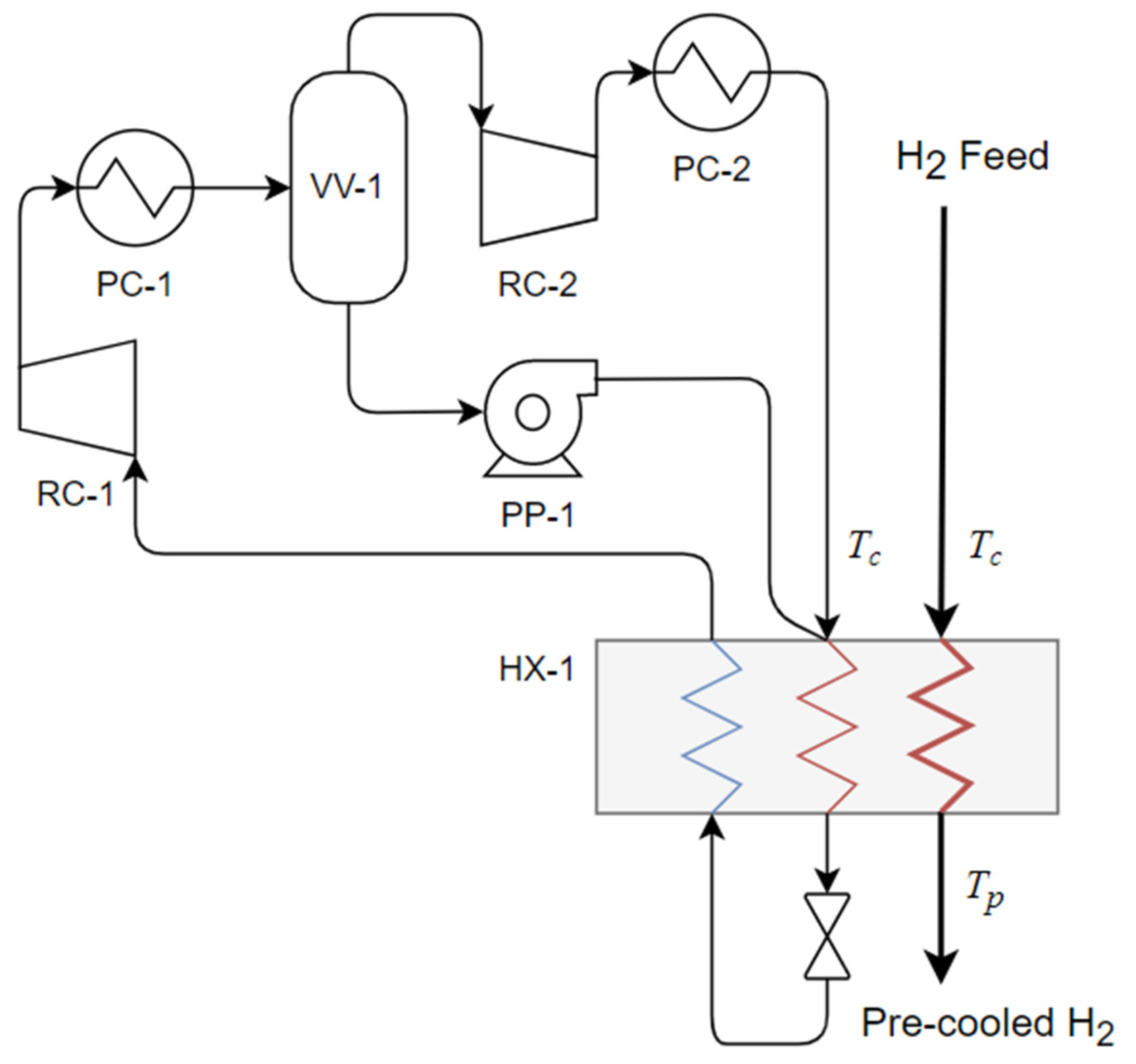
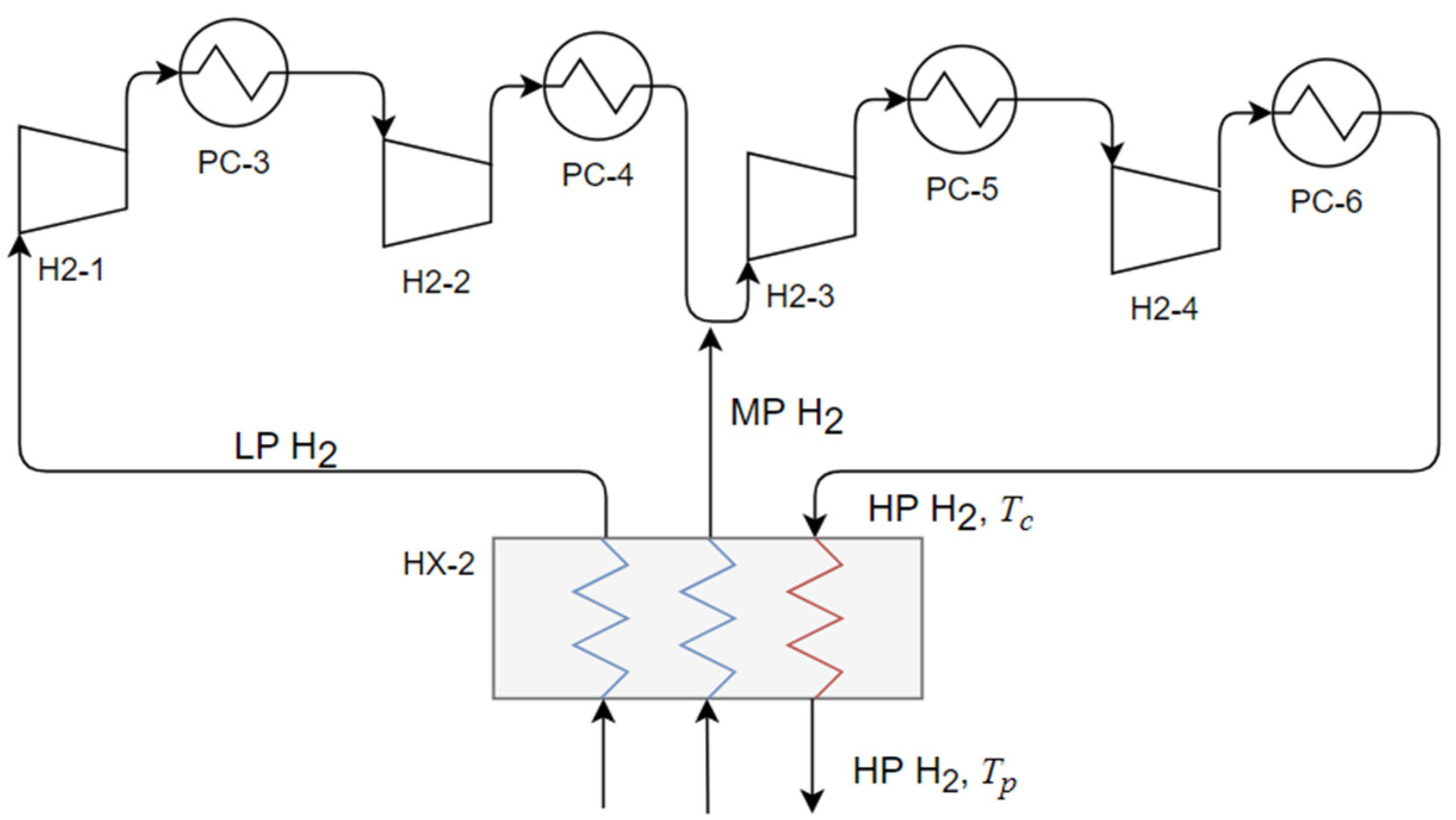
2.2. Process Model Development
2.3. MR Pre-Cooling Model Validation
2.4. Optimization Problem Defenition
2.5. Optimization Algorithm
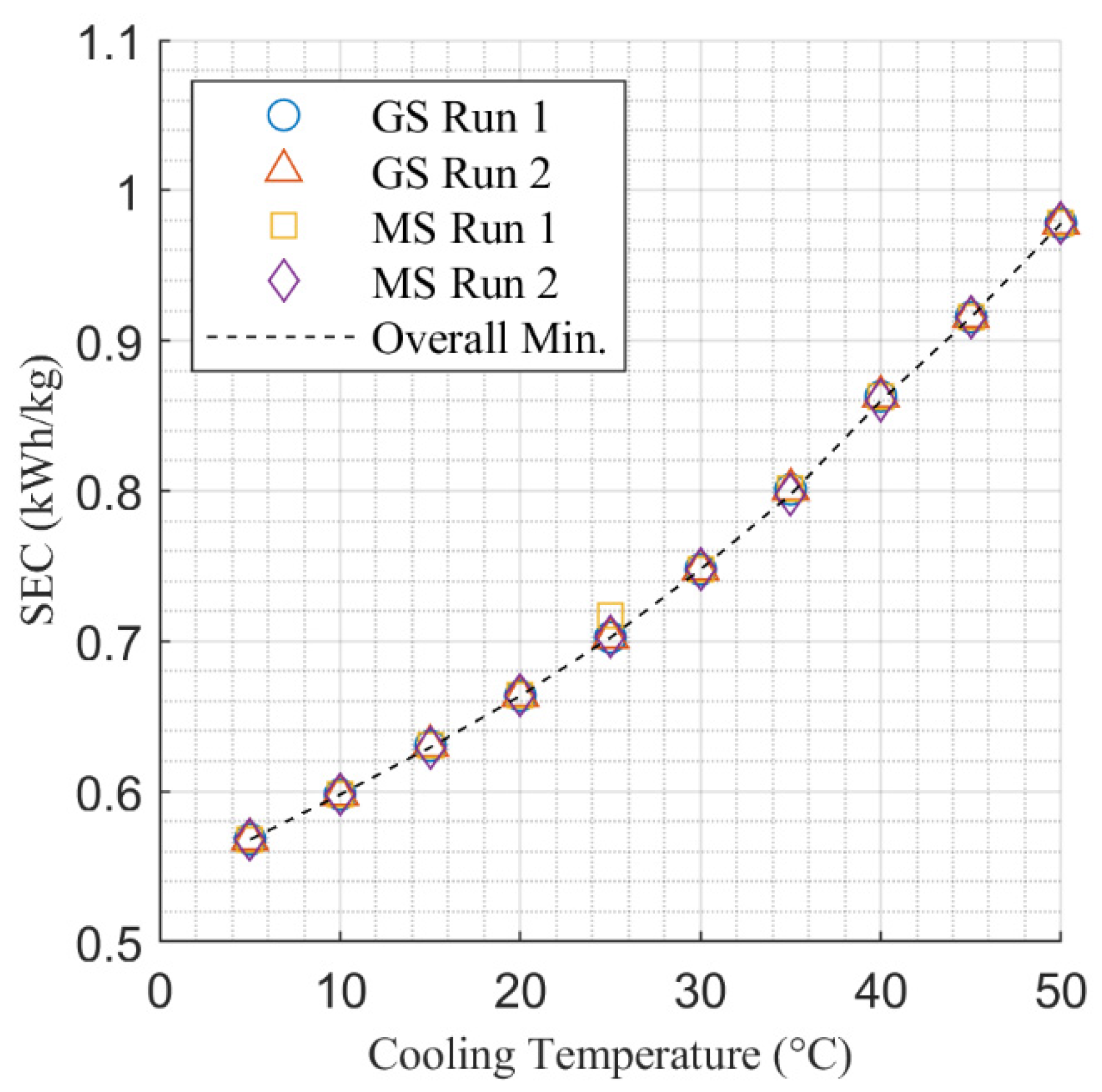
2.6. Performance Variation with Cooling Temperature
3. Results and Discussion
3.1. Process Modelling and Validation
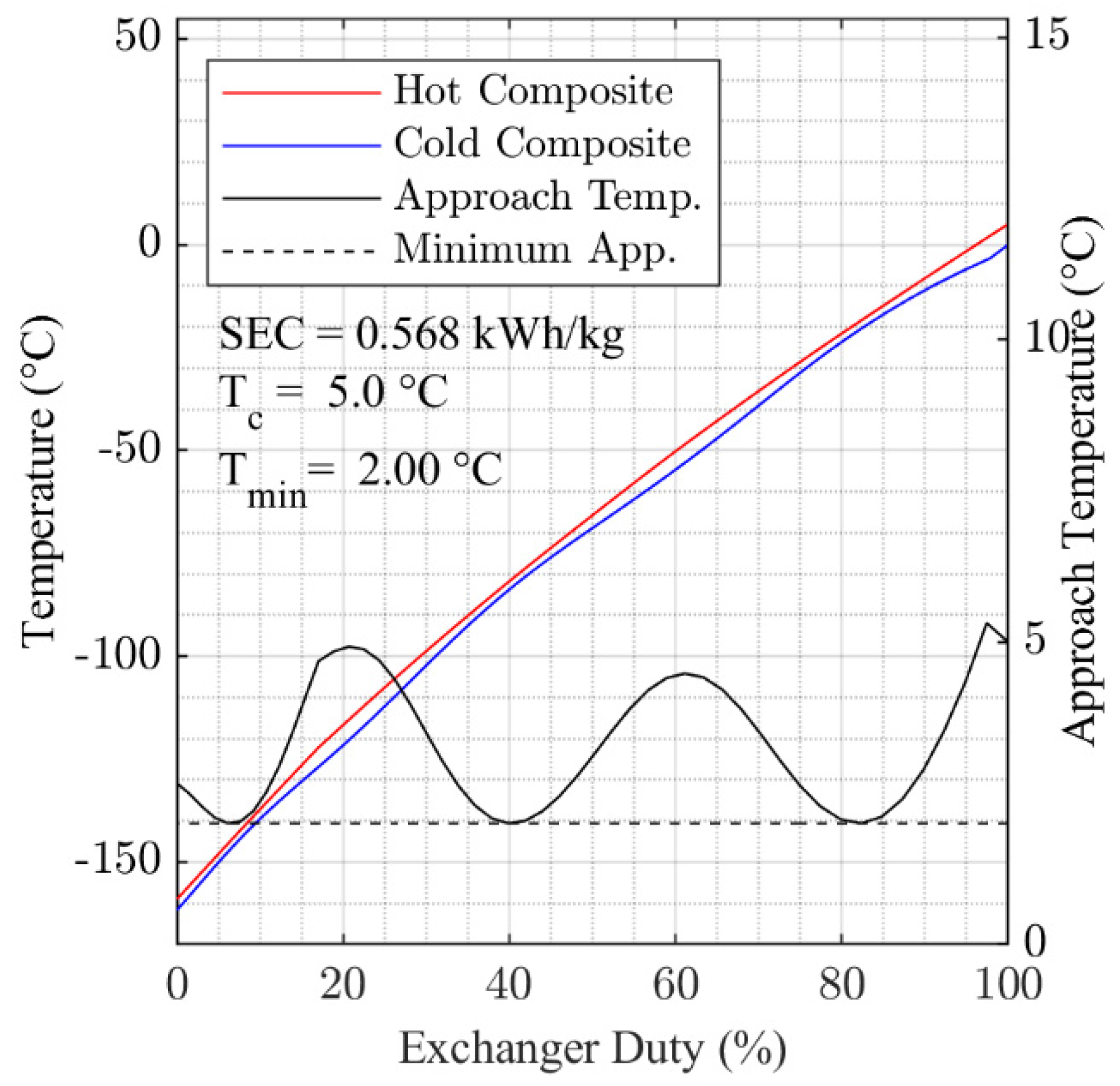
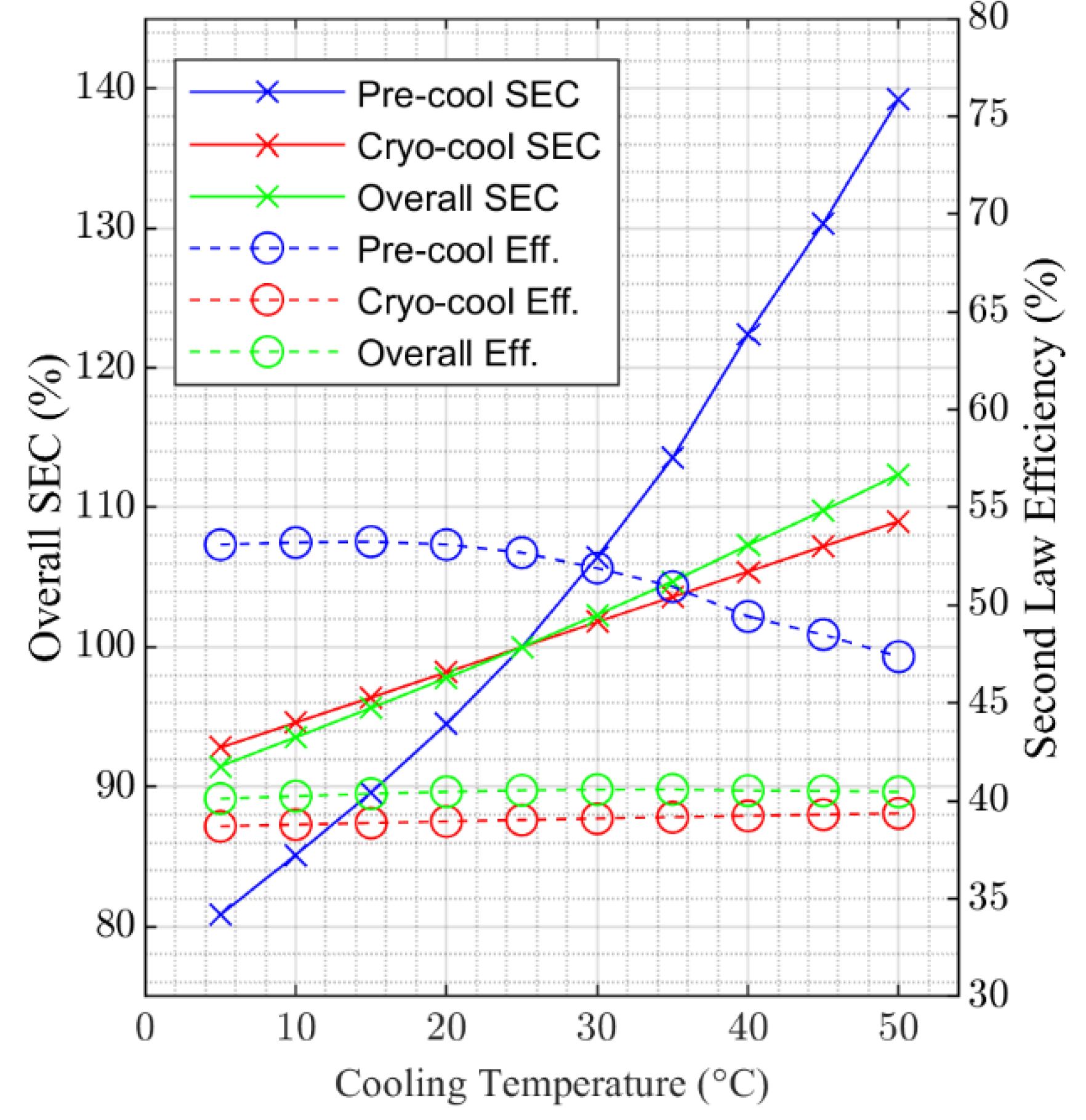
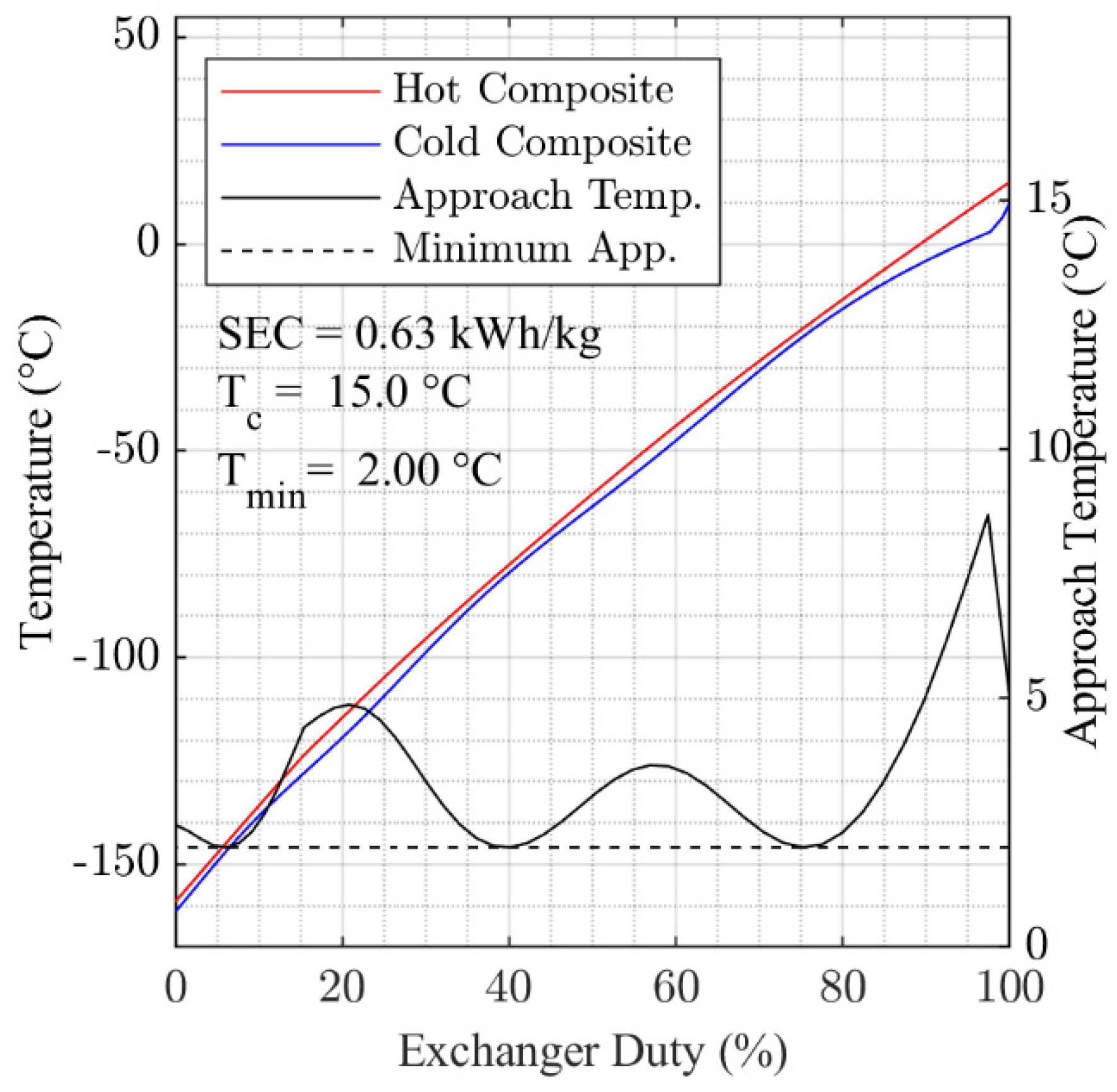
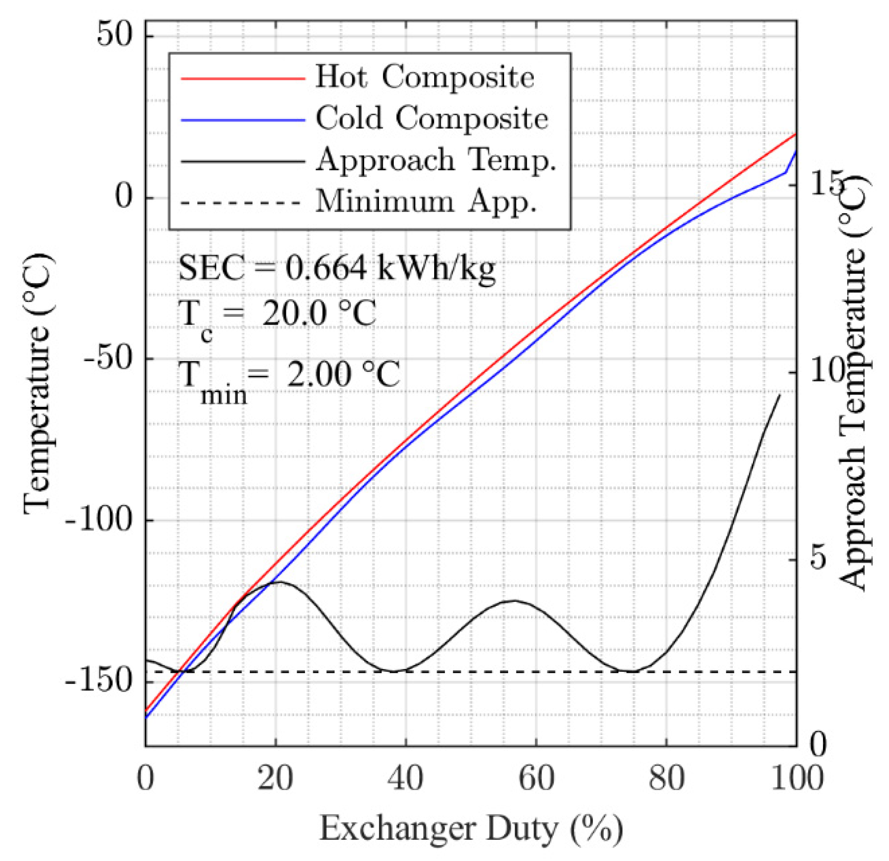
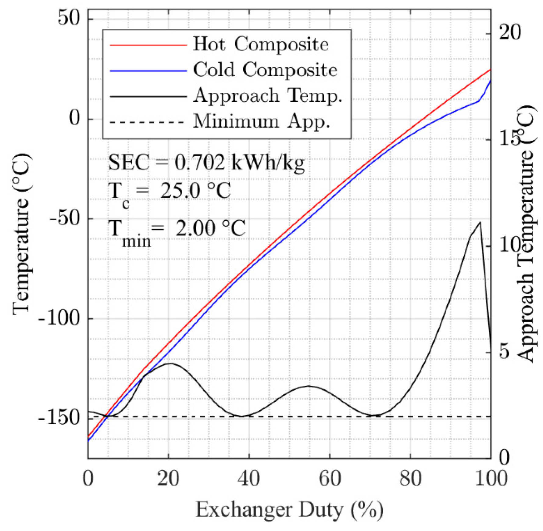
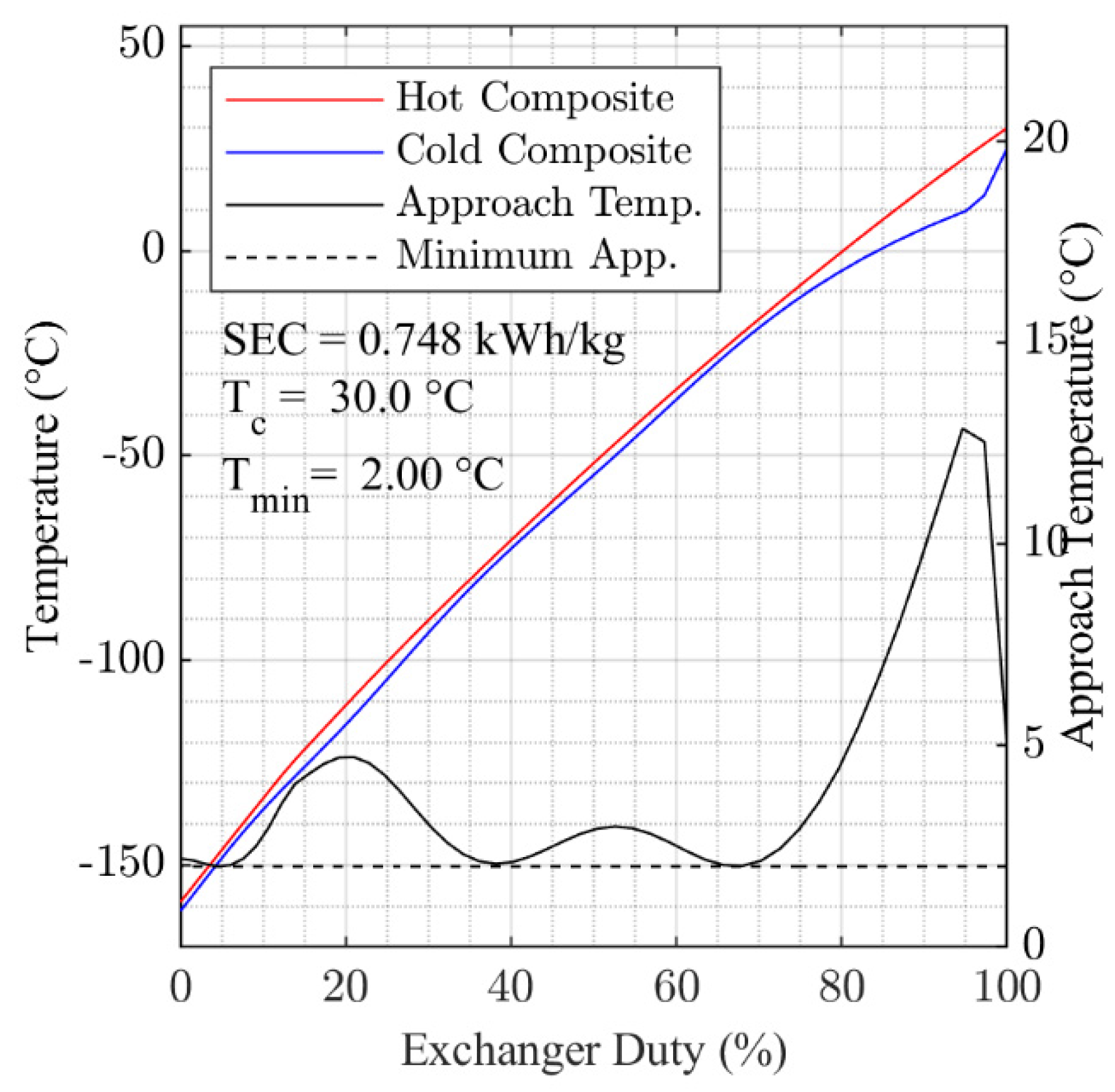
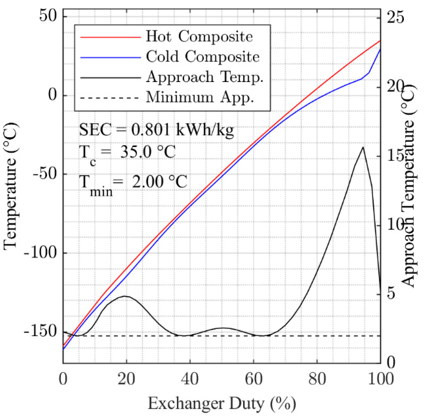
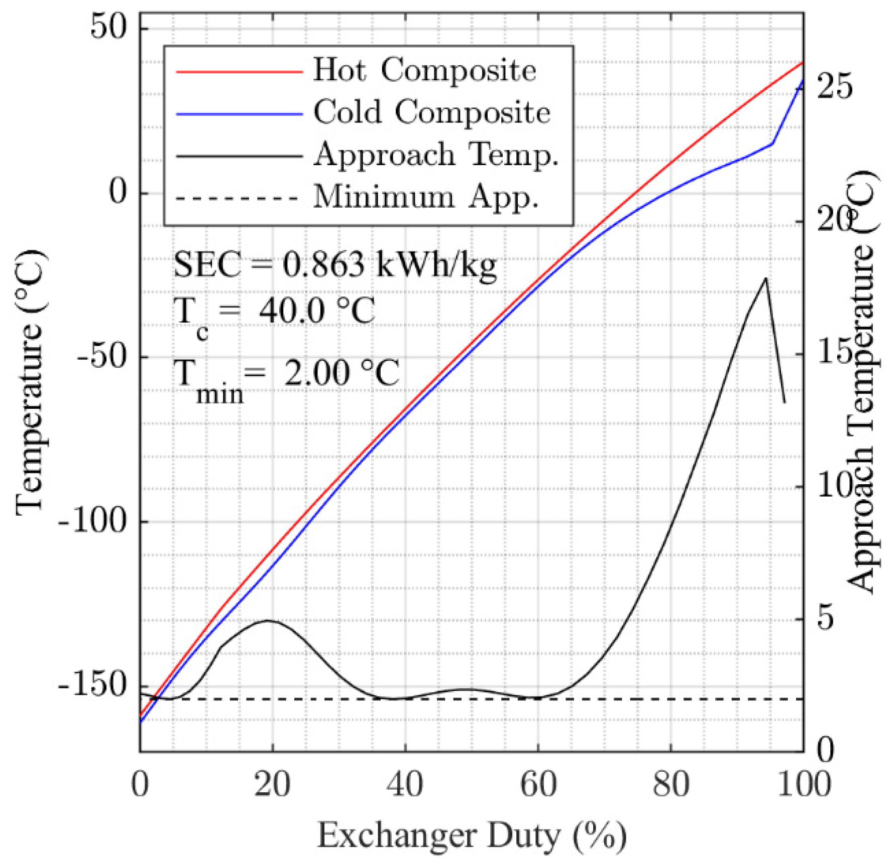
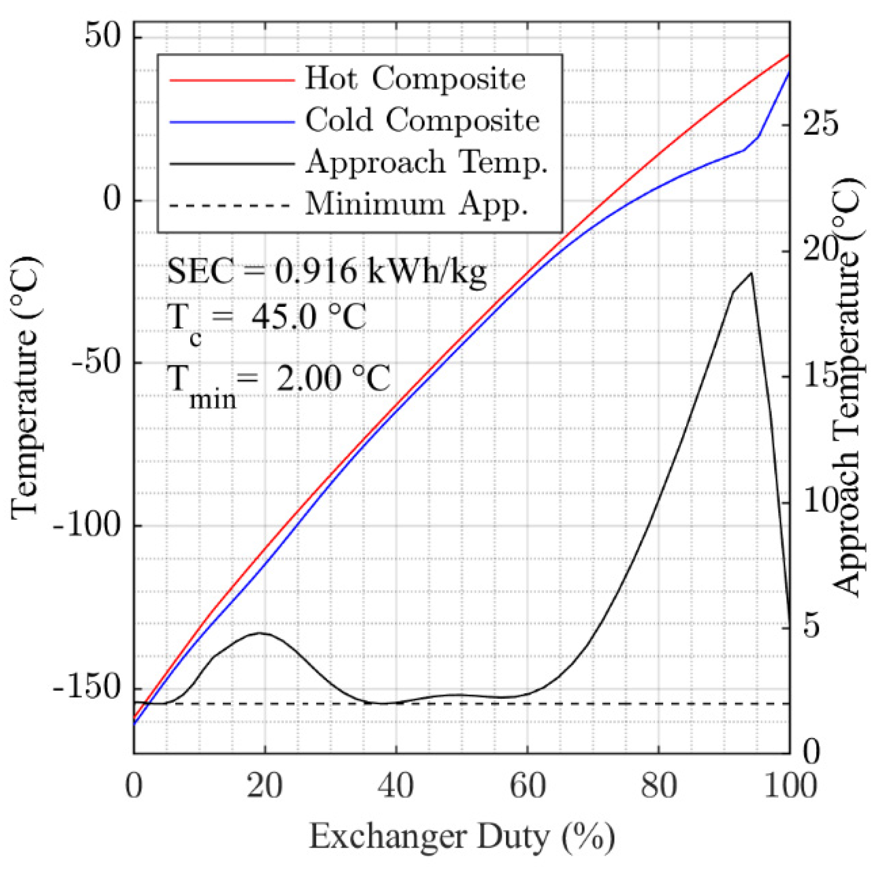
3.2. Performance Variation with Cooling Temperature
4. Conclusions
Author Contributions
Funding
Institutional Review Board Statement
Informed Consent Statement
Data Availability Statement
Conflicts of Interest
Appendix A


References
- Acar, C.; Dincer, I. Review and evaluation of hydrogen production options for better environment. J. Clean. Prod. 2019, 218, 835–849. [Google Scholar] [CrossRef]
- Cell, F.; Undertaking, H.J. Hydrogen Roadmap Europe—A Sustainable Pathway for the European Energy Transition. Fuel Cells Hydrogen Jt. Undert. 2019. [Google Scholar] [CrossRef]
- Moya, J.I.; Dalius, W. Hydrogen Use in EU Decarbonisation Scenarios. Available online: https://ec.europa.eu/jrc/sites/default/files/final_insights_into_hydrogen_use_public_version.pdf (accessed on 1 September 2021).
- The European Comission. A Hydrogen Strategy for a Climate-Neutral Europe; The European Comission: Brussels, Belgium, 2020. [Google Scholar]
- Kang, J.-N.; Wei, Y.-M.; Liu, L.-C.; Han, R.; Yu, B.-Y.; Wang, J.-W. Energy systems for climate change mitigation: A systematic review. Appl. Energy 2020, 263, 114602. [Google Scholar] [CrossRef]
- Yuksel, Y.E.; Ozturk, M.; Dincer, I. Energetic and exergetic assessments of a novel solar power tower based multigeneration system with hydrogen production and liquefaction. Int. J. Hydrogen Energy 2019, 44, 13071–13084. [Google Scholar] [CrossRef]
- Sher, F.; Al-Shara, N.K.; Iqbal, S.Z.; Jahan, Z.; Chen, G.Z. Enhancing hydrogen production from steam electrolysis in molten hydroxides via selection of non-precious metal electrodes. Int. J. Hydrogen Energy 2020, 45, 28260–28271. [Google Scholar] [CrossRef]
- Karakaya, E.; Nuur, C.; Assbring, L. Potential transitions in the iron and steel industry in Sweden: Towards a hydrogen-based future? J. Clean. Prod. 2018, 195, 651–663. [Google Scholar] [CrossRef]
- Pethaiah, S.S.; Sadasivuni, K.K.; Jayakumar, A.; Ponnamma, D.; Tiwary, C.S.; Sasikumar, G. Methanol Electrolysis for Hydrogen Production Using Polymer Electrolyte Membrane: A Mini-Review. Energies 2020, 13, 5879. [Google Scholar] [CrossRef]
- Yang, C.; Ogden, J. Determining the lowest-cost hydrogen delivery mode. Int. J. Hydrogen Energy 2007, 32, 268–286. [Google Scholar] [CrossRef] [Green Version]
- Ishimoto, Y.; Voldsund, M.; Nekså, P.; Roussanaly, S.; Berstad, D.; Gardarsdottir, S.O. Large-scale production and transport of hydrogen from Norway to Europe and Japan: Value chain analysis and comparison of liquid hydrogen and ammonia as energy carriers. Int. J. Hydrogen Energy 2020, 45, 32865–32883. [Google Scholar] [CrossRef]
- Hoshi, M. World’s First Liquid Hydrogen Carrier Ship Launches in Japan. Available online: https://asia.nikkei.com/Business/Energy/World-s-first-liquid-hydrogen-carrier-ship-launches-in-Japan (accessed on 15 April 2021).
- Aasadnia, M.; Mehrpooya, M. Large-scale liquid hydrogen production methods and approaches: A review. Appl. Energy 2018, 212, 57–83. [Google Scholar] [CrossRef]
- Ghorbani, B.; Mehrpooya, M.; Aasadnia, M.; Niasar, M.S. Hydrogen liquefaction process using solar energy and organic Rankine cycle power system. J. Clean. Prod. 2019, 235, 1465–1482. [Google Scholar] [CrossRef]
- Yilmaz, C. Optimum energy evaluation and life cycle cost assessment of a hydrogen liquefaction system assisted by geothermal energy. Int. J. Hydrogen Energy 2019, 45, 3558–3568. [Google Scholar] [CrossRef]
- Ansarinasab, H.; Mehrpooya, M.; Mohammadi, A. Advanced exergy and exergoeconomic analyses of a hydrogen liquefaction plant equipped with mixed refrigerant system. J. Clean. Prod. 2017, 144, 248–259. [Google Scholar] [CrossRef]
- Skaugen, G.; Berstad, D.; Wilhelmsen, Ø. Comparing exergy losses and evaluating the potential of catalyst-filled plate-fin and spiral-wound heat exchangers in a large-scale Claude hydrogen liquefaction process. Int. J. Hydrogen Energy 2020, 45, 6663–6679. [Google Scholar] [CrossRef]
- Cardella, U.; Decker, L.; Sundberg, J.; Klein, H. Process optimization for large-scale hydrogen liquefaction. Int. J. Hydrogen Energy 2017, 42, 12339–12354. [Google Scholar] [CrossRef]
- Yuksel, Y.E.; Ozturk, M.; Dincer, I. Analysis and assessment of a novel hydrogen liquefaction process. Int. J. Hydrogen Energy 2017, 42, 11429–11438. [Google Scholar] [CrossRef]
- Chang, H.M.; Ryu, K.N.; Baik, J.H. Thermodynamic design of hydrogen liquefaction systems with helium or neon Brayton refrigerator. Cryogenics 2018, 91, 68–76. [Google Scholar] [CrossRef]
- Donaubauer, P.J.; Cardella, U.; Decker, L.; Klein, H. Kinetics and Heat Exchanger Design for Catalytic Ortho-Para Hydrogen Conversion during Liquefaction. Chem. Eng. Technol. 2019, 42, 669–679. [Google Scholar] [CrossRef]
- Wilhelmsen, O.; Berstad, D.; Aasen, A.; Neksa, P.; Skaugen, G. Reducing the exergy destruction in the cryogenic heat exchangers of hydrogen liquefaction processes. Int. J. Hydrogen Energy 2018, 43, 5033–5047. [Google Scholar] [CrossRef] [Green Version]
- Skaugen, G.; Wilhelmsen, O. Comparing the Performance of Plate-Fin and Spiral Wound Heat Exchangers in the Cryogenic Part of the Hydrogen Liquefaction Process. In Proceedings of the 15th Cryogenics 2019 Iir International Conference; Prague, Czech Republic, 8–11 April 2019, Chrz, V., Haberstroh, C., Herzog, R., Kaiser, Z., Klier, J., Kralik, T., Lansky, M., Mericka, P., Schustr, P., Srnka, A., et al., Eds.; Refrigeration Science and Technology; International Institute of Refrigeration: Paris, France, 2019; pp. 318–324. [Google Scholar]
- Bauer, H.C. Mixed fluid cascade, experience and outlook. In Proceedings of the AIChE Spring Meeting and Global Congress on Process Safety, Houston, TX, USA, 1–4 April 2012. [Google Scholar]
- Rian, A.B.; Ertesvåg, I.S. Exergy Evaluation of the Arctic Snøhvit Liquefied Natural Gas Processing Plant in Northern Norway—Significance of Ambient Temperature. Energy Fuels 2012, 26, 1259–1267. [Google Scholar] [CrossRef]
- Xu, X.; Liu, J.; Jiang, C.; Cao, L. The correlation between mixed refrigerant composition and ambient conditions in the PRICO LNG process. Appl. Energy 2013, 102, 1127–1136. [Google Scholar] [CrossRef]
- Castillo, L.; Dahouk Majzoub, M.; Di Scipio, S.; Dorao, C.A. Conceptual analysis of the precooling stage for LNG processes. Energy Convers. Manag. 2013, 66, 41–47. [Google Scholar] [CrossRef]
- Park, K.; Won, W.; Shin, D. Effects of varying the ambient temperature on the performance of a single mixed refrigerant liquefaction process. J. Nat. Gas Sci. Eng. 2016, 34, 958–968. [Google Scholar] [CrossRef]
- Jackson, S.; Eiksund, O.; Brodal, E. Impact of Ambient Temperature on LNG Liquefaction Process Performance: Energy Efficiency and CO 2 Emissions in Cold Climates. Ind. Eng. Chem. Res. 2017, 56, 3388–3398. [Google Scholar] [CrossRef]
- Cardella, U.; Decker, L.; Klein, H. Roadmap to economically viable hydrogen liquefaction. Int. J. Hydrogen Energy 2017, 42, 13329–13338. [Google Scholar] [CrossRef]
- The MathWorks, Inc. MATLAB; The MathWorks, Inc.: Natick, MA, USA, 2018. [Google Scholar]
- Span, R.; Eckermann, T.; Herrig, S.; Hielscher, S.; Jäger, A.; Thol, M. TREND. Thermodynamic Reference and Engineering Data 5.0; Lehrstuhl für Thermodynamik, Ruhr-Universität Bochum: Bochum, Germany, 2020. [Google Scholar]


| Parameter | Value | Units |
|---|---|---|
| Hydrogen Feed Pressure | 20 | bara |
| H2 pre-cooling temperature, | −159 | °C |
| Compressor/ pump efficiency | 85 | % * |
| HX-1 pressure-loss (hot streams) | 0.5 | bar |
| HX-1 pressure-loss (cold streams) | 0.1 | bar |
| PC-1 and 2 pressure-loss | 0.5 | bar |
| Parameter | Value | Units |
|---|---|---|
| LP H2 Feed Pressure | 1.1 | bara |
| LP H2 flowrate | 51.5 | tpd |
| MP H2 feed pressure | 8.0 | bara |
| MP H2 flowrate | 1121.5 | tpd |
| HP H2 return pressure | 29.8 | bara |
| PC-3 to 6 pressure-loss | 0.5 | bar |
| Component | Mole Fraction |
|---|---|
| Nitrogen | 0.101 |
| Methane | 0.324 |
| Ethane | 0.274 |
| Propane | 0.031 |
| n-Butane | 0.270 |
| Parameter | Value | Units |
|---|---|---|
| Hydrogen Feed Flow | 125 | tpd |
| MR feed temperature | 12 | °C |
| MR return temperature | −1.0 | °C |
| MR feed pressure | 35 | bara |
| MR return pressure | 4.25 | bara |
| Parameter | Description | |
|---|---|---|
| MR mole fraction N2 | 0.05 < 0.11 < 0.25 | |
| Mole fraction CH4 | 0.20 < 0.32 < 0.50 | |
| MR mole fraction C2 | 0.15 < 0.27 < 0.50 | |
| MR mole fraction C3 | 0.00 < 0.03 < 0.10 | |
| RC-1, Pin (bara) | 2.00 < 4.25 < 6.00 |
| Reference | Case A | Case B | Case C | ||
|---|---|---|---|---|---|
| Properties method | - | PR | SRK | Hel. | |
| MP supply pressure | 35.0 | 35.0 | 35.0 | 35.0 | bara |
| MR return pressure | 4.25 | 3.0 ** | 4.25 | 4.25 | bara |
| MR return temp. | 112 | 112.8 | 112.3 | 109.6 | °C |
| MR mass flowrate | 1600 * | 1395 | 1703 | 1709 | tpd |
| HX-1 min. approach | 1.00 | 1.05 | 0.49 | 0.51 | °C |
| HX-1 duty | 12.6 | 11.2 | 13.2 | 12.9 | kW |
Publisher’s Note: MDPI stays neutral with regard to jurisdictional claims in published maps and institutional affiliations. |
© 2021 by the authors. Licensee MDPI, Basel, Switzerland. This article is an open access article distributed under the terms and conditions of the Creative Commons Attribution (CC BY) license (https://creativecommons.org/licenses/by/4.0/).
Share and Cite
Jackson, S.; Brodal, E. Optimization of a Mixed Refrigerant Based H2 Liquefaction Pre-Cooling Process and Estimate of Liquefaction Performance with Varying Ambient Temperature. Energies 2021, 14, 6090. https://doi.org/10.3390/en14196090
Jackson S, Brodal E. Optimization of a Mixed Refrigerant Based H2 Liquefaction Pre-Cooling Process and Estimate of Liquefaction Performance with Varying Ambient Temperature. Energies. 2021; 14(19):6090. https://doi.org/10.3390/en14196090
Chicago/Turabian StyleJackson, Steven, and Eivind Brodal. 2021. "Optimization of a Mixed Refrigerant Based H2 Liquefaction Pre-Cooling Process and Estimate of Liquefaction Performance with Varying Ambient Temperature" Energies 14, no. 19: 6090. https://doi.org/10.3390/en14196090
APA StyleJackson, S., & Brodal, E. (2021). Optimization of a Mixed Refrigerant Based H2 Liquefaction Pre-Cooling Process and Estimate of Liquefaction Performance with Varying Ambient Temperature. Energies, 14(19), 6090. https://doi.org/10.3390/en14196090