Article

Short-Term Deterministic Solar Irradiance Forecasting Considering a Heuristics-Based, Operational Approach

by
Armando Castillejo-Cuberos
1,*,
John Boland
2 and
Rodrigo Escobar
1,3
1
Escuela de Ingeniería, Pontificia Universidad Católica de Chile, Vicuña Mackenna 4860, Santiago 7820436, Chile
2
UniSA STEM, University of South Australia, Mawson Lakes, Adelaide, SA 5095, Australia
3
Centro del Desierto de Atacama, Pontificia Universidad Católica de Chile, Vicuña Mackenna 4860, Santiago 7820436, Chile
*
Author to whom correspondence should be addressed.
Energies 2021, 14(18), 6005; https://doi.org/10.3390/en14186005
Submission received: 14 July 2021 / Revised: 13 August 2021 / Accepted: 9 September 2021 / Published: 21 September 2021
(This article belongs to the Special Issue Advances in Wind and Solar Farm Forecasting)

Abstract

:
Solar energy is an economic and clean power source subject to natural variability, while energy storage might attenuate it, ultimately, effective and operationally feasible forecasting techniques for energy management are needed for better grid integration. This work presents a novel deterministic forecast method considering: irradiance pattern classification, Markov chains, fuzzy logic and an operational approach. The method developed was applied in a rolling manner for six years to a target location with no prior data to assess performance and its changes as new local data becomes available. Clearness index, diffuse fraction and irradiance hourly forecasts are analyzed on a yearly basis but also for 20 day types, and compared against smart persistence. Results show the proposed method outperforms smart persistence by ~10% for clearness index and diffuse fraction on the base case, but there are significant differences across the 20 day types analyzed, reaching up to +60% for clear days. Forecast lead time has the greatest impact in forecasting performance, which is important for any practical implementation. Seasonality in data gaps or rejected data can have a definite effect in performance assessment. A novel, comprehensive and detailed analysis framework was shown to present a better assessment of forecasters’ performance.

1. Introduction

As installed solar energy capacity increases worldwide, its appropriate management becomes a pressing matter for electric system operators. As more efforts are directed towards further renewable energy integration to established grids, the issue of natural variability of renewable energy becomes concerning. Several studies show that renewable energy dumps due to system operational constraints can be significant and have proposed different dispatch schemes to counter this [1,2]. This does not solve the issue, but complicates it by introducing a new aspect to energy management: appropriate storage and dispatch of energy; hence, solar power forecasting becomes an invaluable tool. To this end, several methods have been developed to produce forecasts and have been presented in comprehensive literature reviews [3,4,5,6,7,8], with statistical methods being very popular.

1.1. Statistical Forecasting Methods: Introduction and Challenges

Statistical methods apply time series analysis to develop forecasts. A general formulation for this family of methods is presented in Equation (1), where Y ( k ) , U ( k ) and e ( k ) stand for the k-th value of the output, input variables and forecast error, respectively. A , B and C stand for the model coefficients that need fitting to match the observations and m, n and p represent the model’s order. When B = C = 0 , the model is called autoregressive (AR), when only C = 0 , the model is called autoregressive with external inputs (ARX) and when C     0 it is an autoregressive moving-average model with external inputs ( B 0 , ARMAX model) or without them ( B = 0 , ARMA model) [9].
A n Y ( k ) +     +   A 0 Y ( k m ) = B n U ( k ) +   + B 0 U ( k n ) + C n e ( k 1 ) +   + C 0 e ( k p )
A procedure presented by Box et al. [10] uses the autocorrelation (ACF) and partial autocorrelation functions (PACF) of the time series, to determine model structure. Since time series can exhibit seasonality, it is often suggested to use the derivative of the time series for the seasonality period, to eliminate this trend and better determine the model’s dynamics, calling such models SARMA (seasonal autoregressive moving average). The core of the methodology is that a particular model (AR/ARMA) exhibits a distinct, identifiable pattern in its ACF and PACF. By identifying the lags in which the ACF and PACF peak or decay, the model order (m/n/p parameters in Equation (1)) can be determined. Finally, linear or nonlinear estimators are employed to determine the model’s coefficients.

1.2. Emergence and Challenges of Artificial Intelligence as Forecasting Tool

Recently, applications of artificial intelligence techniques for solar power forecasting have continually increased due to their ability to model highly nonlinear phenomena and pattern identification, provided by analyzing correlation and clustering between input and output variables [11]. Likewise, Cai et al. [12] present the contrast against conventional statistical techniques, their shortcomings and the emergence of deep learning techniques as a response. These techniques rely on two main concepts: first, identify and classify patterns or features to be reproduced and second, the actual forecast is based on the training of a structure to generate outputs based on the identified pattern to be reproduced. Examples are presented in Table 1 and current issues for these methods on Table 2.
Regardless of the success of these techniques, one issue remains regarding the interoperability of the approach, meaning that the resulting structures are created based on the specific characteristics of the data and the classifier itself is specific to each case of study. Therefore, a generalized classification scheme would benefit the development of forecasting methods by allowing interoperability and ease of implementation and comparison across studies.

1.3. Current State of the Art in Solar Power Forecasting Performance Assessment

Several well-regarded metrics have been presented in the literature for performance evaluation, however, there is not a defined standard on which metrics to report nor how appropriate they are as meaningful indicators of a forecaster’s performance [21]. Furthermore, when comparison against a reference baseline method is required, there may not be an overall agreement on the details of the implementation of such method and there is still debate regarding this topic, to which works such as [22] attempt to set the details for a standardized method. Additionally, as solar power forecasting has transitioned from the naïve persistence (irradiance I remains constant through forecast window, Equation (2), [23,24,25]) towards the smart persistence as the reference method (clear sky index K t c s remains constant through forecast window, Equation (3), [25,26]), the readers must be aware of which reference was used, making analysis and result comparison more difficult.
I ^ ( t + Δ t ) = I ( t )
I ^ ( t + Δ t ) = I c s ( t + Δ t ) ×   K t c s ( t ) = I ^ c s ( t + Δ t ) × I ( t ) I c s ( t )
From this body of knowledge, a baseline can be established regarding the performance of different forecasting methods. Results presented in [6,8] were analyzed considering that: (a) must have been assessed with a minimum of one year of validation data and (b) only hourly forecasts were considered. The normalized root mean square error (nRMSE) was the most commonly reported metric, with typical values in the range of 17 ± 8.25%, although values of 3% and 38% have been reported as well. Figure 1 presents results from selected works [27,28]; however, the reader is referred to [6,8] for a more detailed coverage of performance statistics.
Despite the fact that several well-known metrics and procedures for forecasting performance assessment are presented in the literature, most studies are limited to assessing performance of the entire evaluation period, while some further detail at how performance varies with month or season [16,29,30,31], but comparatively few studies provide details at the type-of-day [15] level or for specific values or ranges for K t [14,32]. This analysis is of interest, because as Figure 1 shows, the same method can yield very different results as a function of the variability of the location under analysis. Often, the type-of-day categories are defined subjectively, and [33] showed that K t alone is not a sufficient metric to characterize day type, proving that these approaches are not sufficient to accurately characterize performance under specific atmospheric dynamics. Further, studies commonly use training–evaluation–testing datasets that, in sum, encompass all of their available data, but rarely evaluate how data aggregation affects forecasting performance, and the testing datasets are frequently composed of few years or even fractions of a year. It is therefore necessary to develop an assessment framework that addresses these shortcomings.
Finally, academic work in this area has mostly been oriented towards developing techniques to increase forecast accuracy. However, recent studies have shown that this approach is insufficient, as there are several critical issues pertaining to implementation and performance assessment that have not been standardized or that have not reached scientific consensus. For the operational aspect of forecasting, the method should be able to be integrated seamlessly in the decision-making process regarding energy dispatch. Yang et al. [34] point to key issues related with database requirements, computational time required to obtain useful results, time difference between forecasted energy and the anticipation on which the forecast must be provided (lead time) and data processing to comply with temporal resolution requirements.

1.4. Present Work and Scientific Contributions

From these arguments, the authors have decided to develop a novel statistical solar forecasting method and a comprehensive assessment methodology, aimed at addressing the issues detected in the literature review. Namely, the novelty and contributions of this work are summarized as follows:
  • A novel solar radiation forecasting method was developed based on pattern identification and classification, probability and heuristic methodology, considering operational needs of decision-making parties. The heuristic method developed for this application presents an intuitive, explainable, interpretable and effective way to forecast solar irradiance, by relying on concepts of probability, possibility and human reasoning, overcoming the limitation of complex mathematical abstraction and black-box characteristics of advanced state-of-the-art statistical and artificial intelligence methods.
  • A generalized explicit irradiance pattern classification scheme was employed for performance assessment and forecasting, by classifying irradiance patterns through an analytical expression that yields similar results to clustering techniques, with the advantage of easy implementation across studies.
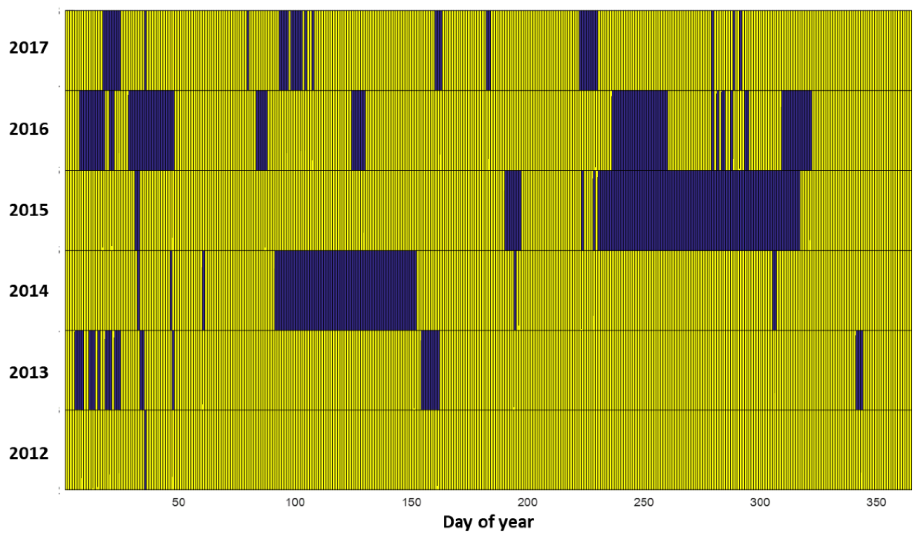
  • A comprehensive performance assessment framework was developed to analyze not only how forecasting performance changes as a function of forecast horizon and lead time, but to evaluate the effect of data aggregation into the knowledge base has on forecasting skill, how quality control and/or data gaps affect performance assessment and how the forecaster performs under different objectively defined day types.
This work is organized as follows: Section 1 deals with the introduction and a brief state-of-the-art description in the issues relevant and under study in solar radiation forecasting. Section 2 presents the data sources and explains the forecasting methodology and Section 3 deals with performance assessment methodology. Finally, the fourth section presents the results and discussion, and Section 5 presents the conclusions.

2. Data Sources and Methodology

Data corresponds to seven measurement stations throughout Chile (Arica, La Tirana, Crucero, Diego de Almagro, Carrera Pinto, Santiago and Curicó), from 2012 to 2017 with one-minute temporal resolution, integrated to obtain hourly data. Measurement station location, data availability and quality control scheme are detailed in [33,35]. The ESRA clear sky model [36] was used due to its simplicity and accuracy, showing good agreement with ground measurements [35].
While conventional statistical methods have been extensively employed for solar power forecasting, as described in the introductory section, these models are more suited to accurately reproduce the dynamics of a system whose nature/parameters do not change significantly. When this is not the case it is necessary to repeat the fitting procedure to match the new dynamics. This poses not only a complexity to maintain an updated model, but also because very different dynamic patterns can emerge even within the same range of static characteristics (i.e., for the same mean K t c s for a given period, wildly different irradiance patterns can occur), a statement supported by [19,37].
Figure 2 illustrates this conundrum. The top-left subfigure displays the probability a particular one-minute value for K t c s occurs for 20 possible categories with similar hourly K t c s and the top-right subfigure presents the one-minute time series of K t c s values for a representative time series of the corresponding category. By applying the Box–Jenkins methodology to identify which model structure would be the most appropriate, very different ACF and PACF patterns emerge for each time series that represents the different K t c s patterns (shown in the bottom subfigures). Therefore, different structures would need to be developed for each pattern (with additional uncertainty, as different patterns can exist within the same K t c s class) and an additional effort would need to be made to correctly identify transitions across patterns. Ultimately, no one-model-fits-all approach can be employed and similar results are obtained for hourly time series.
Based on the previously discussed limitations of conventional statistical techniques, and the more modern artificial intelligence/deep learning approaches, and considering that the short-term variability of the solar resource is inherently stochastic in its origin, a probability-oriented approach, through Markov chains, is suited to represent these phenomena as the probability distribution to transition from a defined origin state to a destination state in the future, or simply, a chain of connected states [6]. In this way, the problem is first shifted to define the characteristics of such states, then to quantify their transitions and finally to resolve a point value within the destination state.
Examples of this approach are presented in Bhardwaj et al. [38], where Markov chains were used to model transitions for atmospheric variables (temperature, humidity, sunshine hours, atmospheric pressure and wind speed) and a generalized fuzzy model was developed to take these variables as inputs to produce solar irradiance as the output. Sanjari and Gooi [39] produced probabilistic forecasts for photovoltaic plants as a function of irradiance, temperature and the plant’s previous production, using a Markov model. Clusters for different patterns for inputs were constructed based on data similarity using either a shape similarity approach [38] or a pattern discovery method [39]. While these approaches proved successful, the method is highly dependent on the characteristics of the data, as the resulting clusters are defined based on mathematical abstractions and no straightforward relations allow for simple understanding of the data characteristics and cluster boundaries, but more importantly, the interoperability or how the resulting construct can be applied to a different context, a shortcoming shared by [13,14,15] and already expressed in the introductory section.
However, in Castillejo-Cuberos and Escobar [33] it was determined that the overall specific static and dynamic characteristics of solar irradiance for a determined time period, or state, are summarized by the clearness index ( K t ), the diffuse fraction (K) and the variability of the solar resource. By defining a variable termed the solar resource quality score (QS), irradiance patterns can be classified in an explicit scheme comparable to clustering techniques, but providing a straightforward approach and a simple analytical expression on which to perform the classification, easily translatable across studies, overcoming the issue of data specificity previously discussed. The only variables needed are the global horizontal irradiance (GHI), diffuse horizontal irradiance (DHI) and extraterrestrial irradiance ( I o ).
The QS is a measure of how close a particular state is from the ideal of full atmospheric clearness ( K t = 1), no attenuation (K = 0) and constant irradiance (variability = 0). To quantify variability, the variability score ( V S c d f ) defined by Lave et al. [40] was used, defined as the probability that a particular ramp rate ( R R = d G H I / d t ) exceeds a given threshold ramp ( R R 0 = 1000   W / m 2 ) during an evaluation period. The quality score uses the normalized V S c d f or n V S c d f , which is the result of linearly mapping the V S c d f from the range 0.002–0.4054 to 0–1 [33].
K t = G H I I o
K = D H I G H I
V S c d f = min ( ( R R R R 0 ) 2 + ( P ( | R R Δ t | > R R 0 ) 1 ) 2 )
Q S = 1 ( 1 K t ) 2 + ( K ) 2 + ( n V S c d f ) 2 3
In [33], solar resource patterns were classified in 20 classes (or states) from overcast to cloudless (Figure 3). From the time series of hourly K t , K and V S c d f values, an hourly time series of these discrete states can be constructed after applying this classification scheme.
Then, to model the probability that a particular state could develop into another at a future time, transition matrices are constructed from these data. Since the actual physical phenomenon (irradiance time series) would now be represented by a continuous series of discrete states (irradiance classes) then, for each time instance (hour), the following state would only be a function of the previous one, for which assuming a perfect forecast, it would amount to a one-hour forecast horizon. As the lead time is a construct that results from the operational need to know future states with enough anticipation to prepare and enact appropriate measurements, it is not part of the physical reality of the phenomenon to be modeled and its value is determined by the specific need of the end user of the forecast.
Thus, given these two temporal parameters, there are infinite combinations of forecast horizons and lead times on which the transitions could be modeled. Therefore, striving to reproduce the atmospheric dynamics that govern solar resource patterns in a simple yet general way and based on the consideration that each state only depends on the previous one, the probability of transition is modeled corresponding to a forecast horizon of 1 h and no lead time.
Then, the probability of transition is modeled based on historical values by means of transition matrixes, in which for each hour, the preceding state (i.e., irradiance class) is compared against the current one, and the corresponding transition is added to a totalization matrix. Once this process is completed, the counts are normalized across origin states as to obtain the transition probability distribution from each origin state to each end state. This process is presented in Figure 4 where P ( i , j ) represents the probability to transition from “i” origin state towards “j” destination state.
However, this procedure does not consider the relationship of irradiance patterns with solar geometry and seasonality, as the same solar elevation (α) can correspond to very different times of day across stations due to the effect of declination. To capture these seasonality effects (intradaily and intermonthly), transition matrices are developed for nine cases: for α, (in increments of 30°) and hour angle ( ω h ) according to sunrise and sunset angles ( ω s r and ω s s , respectively) for the following sets: (i) ω h < 0.5   ω s r , (ii) 0.5   ω s r 0.5   ω h < 0.5   ω s s and (iii) 0.5   ω s s     ω h .
Once the irradiance class origin/destination probability distribution is known, what follows is to determine the corresponding deterministic forecast. As the K t and K distributions overlap for more than one irradiance class (Figure 3), the complexity of the reversion process increases. To deal with this complexity, while maintaining human interpretability and experience into the process, a fuzzy logic approach was employed, as in [38].
Fuzzy logic, proposed by Zadeh [41], is a framework of multivariate logic that aims at translating human reasoning of imperfect logic with uncertainty. Instead of dealing with all true or false affirmations of binary logic, fuzzy logic evaluates how “accurate” is a particular affirmation by considering the membership degree of an input to a linguistic affirmation that is translated into a fuzzy rule. In [42,43,44,45] it is established that fuzzy logic is compatible with, although distinct to, probability theory in a framework of possibility, the main difference being that probability is concerned with “what will happen” while possibility refers to “what can happen”. This compatibility, the ability to approach the reasoning process from an inherently uncertain point of view, and the fact that a possibility framework is compatible with discrimination against scenarios that are physically impossible (i.e., a K t = 1 with K = 1), makes the fuzzy logic approach suitable for this work.
Barragán [46] explains in detail the mathematical foundation of fuzzy logic in a comprehensive manner and the reader is referred to this work should a high level of detail be needed; however, Figure 5 presents a summary of the procedure. First, numeric values for variables are compared against affirmations or rules (membership functions) to determine their degree of membership to a particular affirmation, resulting in a fuzzy number representing this membership. In the second stage, all affirmations are aggregated using fuzzy logic set operators (such as addition, product, intersection or negation) to establish the current state of affairs in the system under analysis. Then, using a series of rules that constitute the knowledge base of the fuzzy logic system and have been defined either by previous experience and/or human expert knowledge, an inference is made regarding the most appropriate or likely outcome. Finally, since all this process is performed using fuzzy numbers, it is necessary to translate the results back to a crisp numerical value, in a process called de-fuzzification.
The concept of set membership is taken from fuzzy logic to assess the membership degree of a Kt-K-QS value to a certain irradiance class and Figure 6 presents the workflow for each variable, using QS as example. First, the variable is evaluated using Gaussian membership functions defined for each of the 20 defined classes presented in Figure 3 to determine the most similar class or origin state (Figure 6a). Then, the transition probability distribution corresponding to the origin state (Figure 6c) is extracted from the general transition matrix (Figure 6b). This distribution represents the probability of transition from the current origin state to the destination (or forecasted) state. Equation (8) presents the Gaussian membership function in which x refers to the variable to be tested, μ x and σ x represent the mean and standard deviation of the set, respectively.
G M F = e x p ( ( x μ x ) 2 2 σ x 2 )
Since each destination state has a range of values defined by the corresponding mean and standard deviation of its irradiance class (Figure 6d) and there is a definite probability of occurrence for each state, the overall likelihood of a particular value being realized depends upon a combination of these two facts. This relationship can be expressed through the product operator, and therefore the fuzzy “likelihood” variable is defined as the product of the probability of occurrence of a state and the degree of membership for a variable’s values for each state (Figure 6e). Since there are still a multitude of destination states in which the forecasted variable could be realized between one or another, the algebraic sum of the fuzzy sets corresponding to each origin state results in the overall likelihood function for that variable (Figure 6f).
Equation (7) shows the relationship between these variables; therefore, a Kt-K-QS space exists for a given V S c d f (Figure 7a) and the forecast output must belong to it. Since V S c d f is used to describe the intrahourly variability, has a wider distribution of values and has the least effect in QS compared to K t and K [33], for this work it has been assumed that the intrahourly variability is preserved across hours. With this V S c d f value, the Kt-K-QS space is constructed (Figure 7b) and using the previously determined QS likelihood function (Figure 7c) the Kt-K-QS space can be mapped into the QS likelihood function in the Kt-K space (Figure 7d).
However, certain Kt-K combinations violate physical irradiance limits, for which no forecast can be produced. Hence, there exists a binary plausibility space (Figure 7e) representing this (1 for plausible and 0 for implausible values), with K t and K limits being derived from the irradiance limits for GHI, DHI and direct normal irradiance (DNI) established by [47,48] calculated at the forecast’s corresponding α and I o . The last space to consider is constructed from the likelihood functions of K t and K (Figure 7f). Finally, the product operator is used to aggregate the QS likelihood space, the combined K t -K likelihood and the plausibility space, to obtain the overall combined likelihood in the K t -K-QS space, representing the overall likelihood for the combination of variables. To obtain the crisp numerical K t , K and QS values, a centroid defuzzification has been chosen, as this criterion considers the information of all the space and not just the maximum value.
Once the K t and K forecasts have been obtained, the corresponding irradiances are calculated using Equations (4), (5) and (9). Since the application of interest is power forecasting for photovoltaic plants, the tilted plane irradiances are calculated for fixed (at latitude), one and two-axis tracking surfaces, using the HDKR transposition model [49], with a ground surface albedo of 0.2.
D N I = ( G H I D H I ) sin α
For performance assessment, the proposed method is compared against smart persistence (persistence henceforth) as it is the current reference method. To reduce forecast uncertainty due to the clear sky model, especially in cases of marked changes in Linke turbidity during nonclear conditions (as demonstrated in [35]), K t will be used instead of K t c s . As stated in Section 1, persistence forecasting as consensus baseline method has transitioned from naïve persistence (i.e., irradiance remains constant, Equation (2)) [23,24,25] towards smart persistence (i.e., clear sky index remains constant, Equation (3)) [25,26]. However, the estimation of the clear sky irradiance is subject to astronomical uncertainties (solar geometry modeling, Earth–Sun distance modeling and solar constant estimation uncertainty), atmospheric properties uncertainty (such as aerosol optical depth and integrated water vapor column estimation, among others, with specific effects depending on the clear sky model being used) and the intrinsic clear sky modeling error (which is model dependent). Even under perfect circumstances in which these parameters are estimated with low uncertainty on clear days, the clear sky modeling error can amount to ~2–3% for GHI and ~8% for DNI [50] and [51] further elaborates on the sensitivities of clear sky models to uncertainty in their inputs. Finally, in [35] it was shown than under practical applications, it is difficult to maintain accurate and updated estimates of atmospheric properties used for clear sky modeling, that can result in significant estimation errors.
Therefore, in order to reduce forecast uncertainty due to clear sky modeling, the clearness index ( K t ) will be used instead of the clear sky clearness index ( K t c s ) for GHI persistence forecasts, as the former is much less subject to uncertainty than the latter, as it is only affected by the astronomical uncertainties. Likewise, the corresponding DHI forecast stems from this GHI forecast and assuming persistency of the diffuse fraction. For consistent evaluation, the persistence forecasts will be subject to the physical limit constraints previously described.
Data are grouped into two sets: a training set consisting of all but the last year and the evaluation set consisting of the last year. Data for the seven measurement stations are considered, however, to assess the performance of the proposed method, the Santiago station is the one to be analyzed. First, it will be assumed that no previous data for this station exist and then, gradually, data from each additional year are considered for the training set, to simulate data availability once the forecasting scheme is put into operation.

3. Assessment Methodology

The proposed method’s performance is assessed through a set of commonly used error metrics featured in the literature, as reported by [21,34,52], namely, the mean bias error (MBE), the root mean square error (RMSE), the normalized root mean square error (NRMSE), the mean absolute percent error (MAPE), the time series correlation ( ρ ) and the skill score (SS).
M B E = i = 1 i = n e i n
R M S E = ( i = 1 i = n e i 2 ) n
N R M S E = R M S E I o b s e r v e d ¯
M A P E = 100 × ( i = 1 i = n | e i | ) n
ρ = i = 1 i = n ( ( I f o r e c a s t i I f o r e c a s t ¯ ) × ( I o b s e r v e d i I o b s e r v e d ¯ ) ) i = 1 i = n ( I f o r e c a s t i I f o r e c a s t ¯ ) 2 × i = 1 i = n ( I o b s e r v e d i I o b s e r v e d ¯ ) 2
S S 1 R M S E t e s t e d _ m e t h o d R M S E r e f e r e n c e _ m e t h o d
Since module capacities are reported at standard testing conditions (STC, 1000 W/m2 ≅ 25 °C) and plants vary in capacity, it is reasonable to estimate electric power production as the product of the nominal production capacity by the irradiance on the module’s surface and reference the error metric to the nominal plant capacity C n o m i n a l , following [32]. Therefore, the errors are calculated as follows: e i r r for irradiance, while e p o w e r for power production at tilted plane cases. Only valid data points that passed quality control are considered for error calculation.
e i r r = I f o r e c a s t I o b s e r v a t i o n
e p o w e r = C n o m i n a l I f o r e c a s t C n o m i n a l I o b s e r v a t i o n C n o m i n a l I o b s e r v a t i o n = I f o r e c a s t I o b s e r v a t i o n I o b s e r v a t i o n

4. Results and Discussion

4.1. Data Aggregation Effect on Forecasting Performance

The reference case, Santiago 2012 with one-hour forecast horizon and no lead time, proves the proposed forecasting methodology generality by resulting in positive SS, despite not having previous information of this location’s dynamics. As additional data become available, performance increases for the first year of new data and continues to improve with each passing year. Forecasting performance for GHI is closely tied to K t , while for DHI is more complex, as it compounds the forecasting error of K with K t , therefore results are larger than GHI alone. Since DNI is calculated from GHI, the good GHI forecasting performance is carried over to DNI.
As tilted plane irradiance can be considered a weighted sum of the three components, with variable weights according to solar geometry, individual component forecast errors can be somewhat balanced by the others, resulting in a more uniform performance (Figure 8, right). Two-axis tracking forecasting performance is highest among tilted planes, as it depends more upon DNI due to the negligible angle of incidence, whereas fixed plane and one axis tracking have performance close to K t /K levels.
The method tends to perform worst around sunrise due to changes in atmospheric dynamics occurring during the night, potentially resulting in considerable forecasting errors for the sunrise forecast window. Figure 9 presents the actual and forecasted time series for K t , K and irradiances on one completely clear day, one clear with a slightly higher K and variability, and the third one is very variable, having overcast, intermediate and clear periods. For the first day, the forecast was accurate with only DNI overestimation towards sunset due to a combination of overestimation of K t and underestimation of K. This propagated into the tilted irradiance forecast, especially for the two-axis tracking case due to its higher dependence on DNI. The forecast for the second day was accurate as well.
The third day showcases the worst performing situation: when the conditions of the first hour to be forecasted on a day are significantly different than the last forecasted hour of the previous day. The last forecast corresponded to clear sky, which due to unavailability of data in the night hours suggests clear skies during sunrise. During the night the situation changed into an overcast morning resulting in large forecasting error. As daytime data become available, the forecast is rapidly corrected, reducing error.
Once the effect of data aggregation on forecasting performance has been studied, the effect of forecast horizon and forecast lead time can be studied. For this analysis, the training data will consider up to Santiago 2016 data and evaluate performance for 2017 at up to 4 hours’ horizon with up to 2 h lead time.

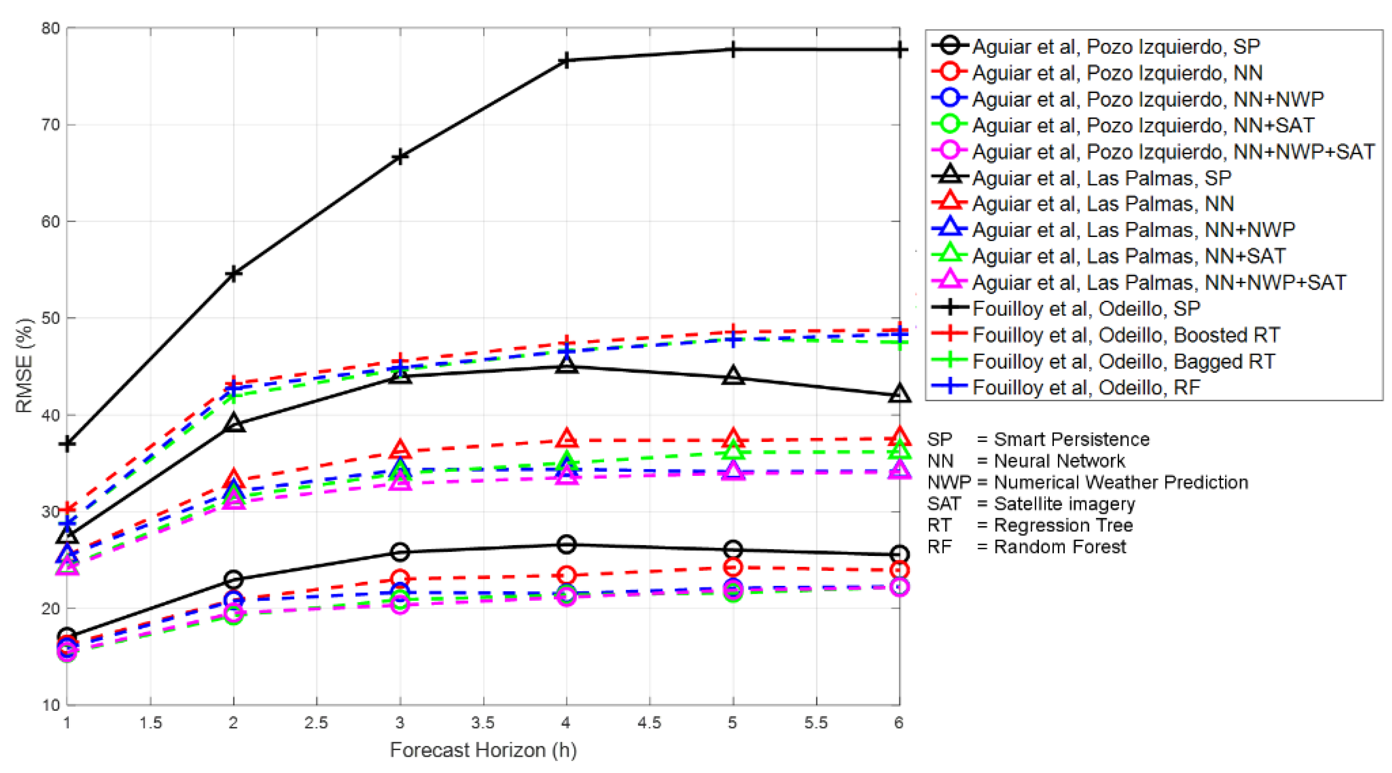
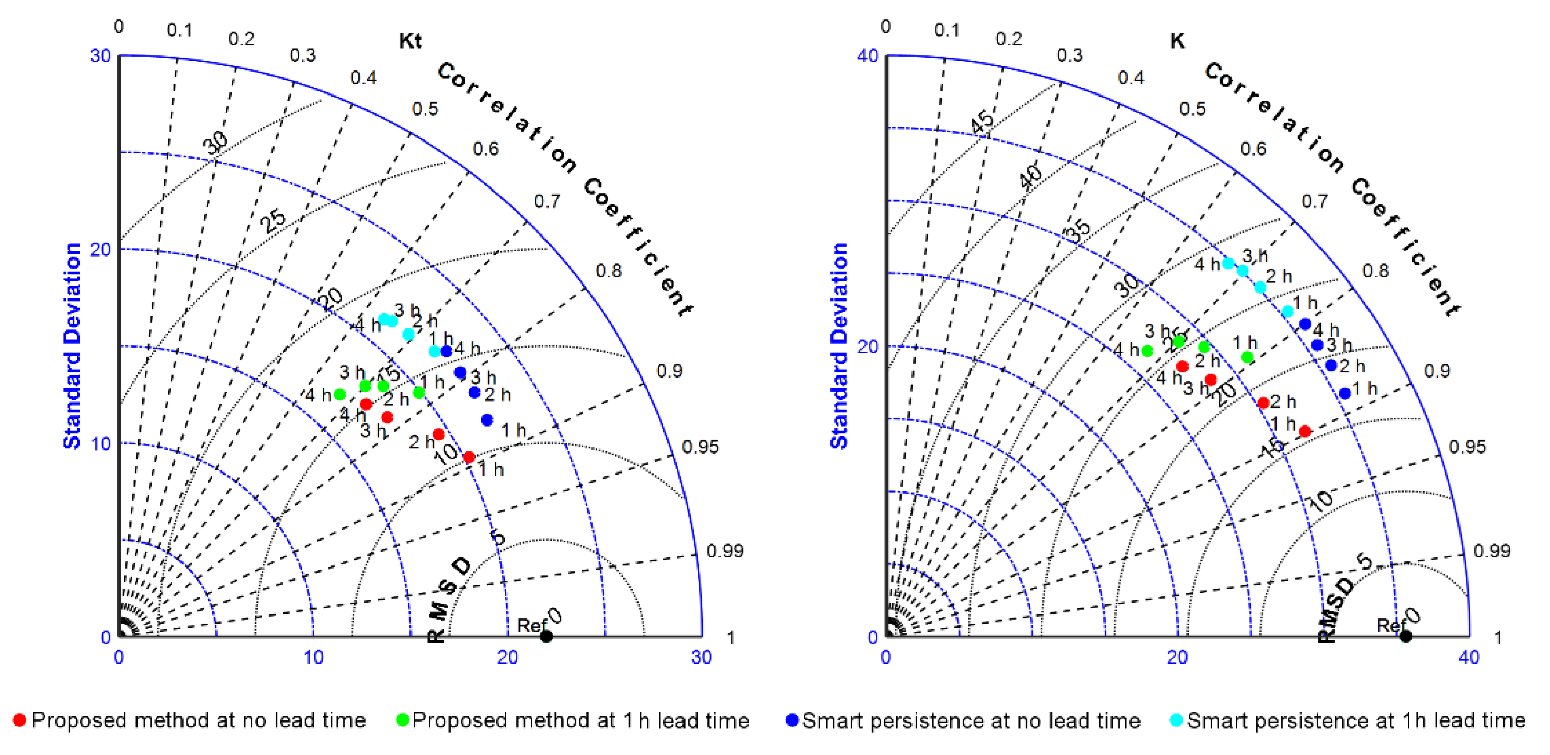
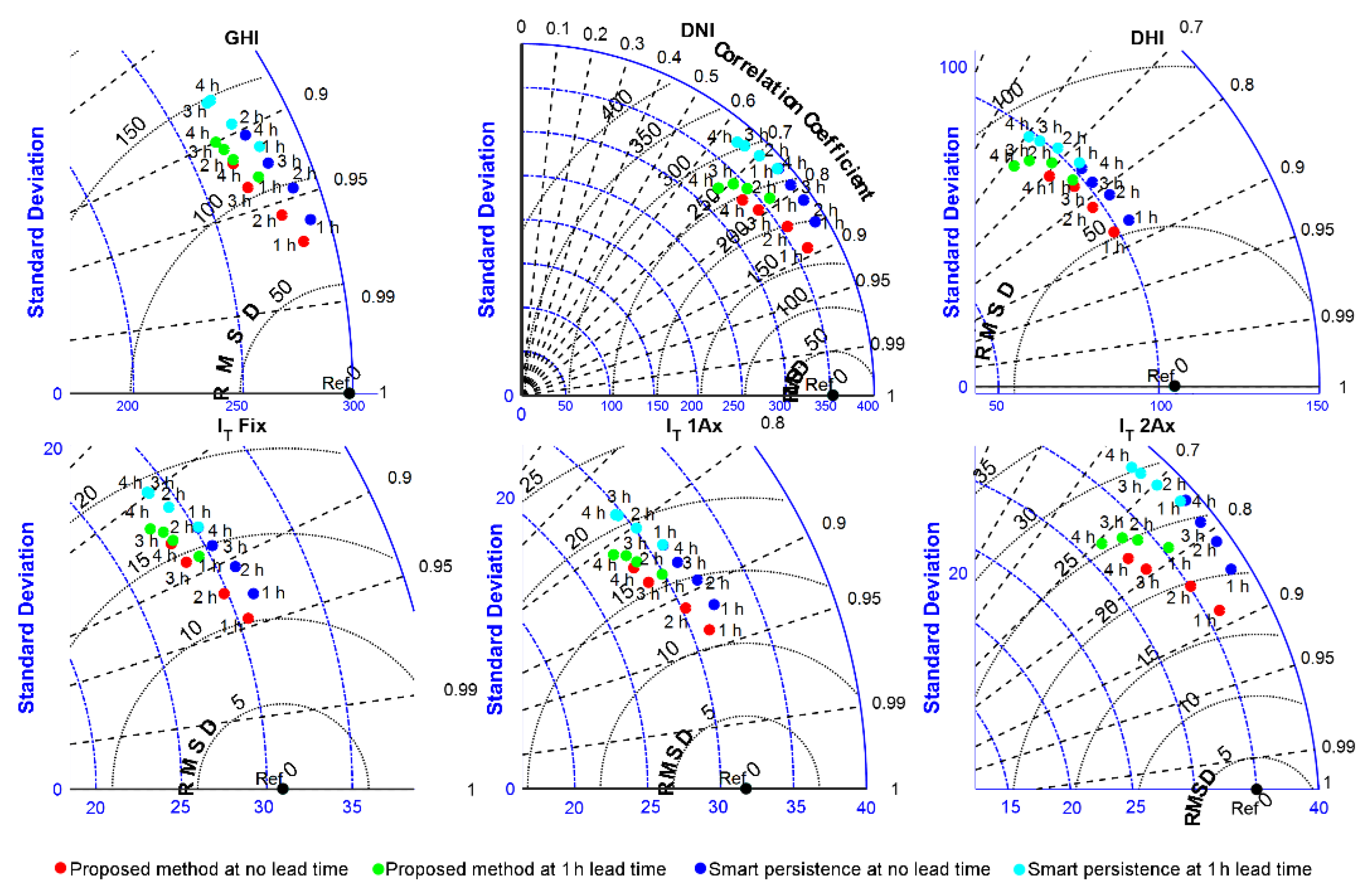
4.2. Effect of Forecast Horizon and Lead Time in Forecasting Performance

Despite the knowledge base being based on historic hour-to-hour transitions with no lead time, the results show the proposed forecasting methodology can be extended for longer time horizons and lead times. From Figure 10, the proposed method showed resistance to performance degradation as the forecasting horizon and lead time increases, with K being the only exception to this behavior. For no lead time cases, the proposed method produces useful forecasts for up to a two-hour forecast horizon while its overall skill is best for the 3 h forecast horizon with a lead time of one hour.
To analyze the detailed performance metrics for each case, Taylor diagrams are chosen. They allow a more detailed, independent analysis for each case, as they summarize several metrics in a single chart based on the relationship presented in Equation (18) [53]. In this diagram, forecast performance is presented as distance to the observations (reference) set, which is perfectly correlated and has no error with itself ( σ r e f e r e n c e   s e t , ρ = 1, RMSE = 0). The farther away from the reference a case is, the performance is worst. For the sake of clarity, only cases of 0–1 h lead times are presented.
c R M S E 2 = σ r e f e r e n c e   s e t 2 + σ t e s t   s e t 2 2 × σ r e f e r e n c e   s e t × σ t e s t   s e t × ρ c R M S E 2 = R M S E 2 M B E 2
Figure 11 presents results for K t and K forecasts. Data points for persistence tend to follow the corresponding standard deviation isoline, due to the persistence forecast being a shifted version of the original time series with increasing decimation as forecast horizon and/or lead times extends. The resulting time series tends to keep most of the distribution characteristics of the original; however, correlation lowers and therefore RMSE increases, with the lead time having the most significant effect. This chart evidences the good performance in forecasting skill for the proposed method, as the increase in the RMSE is lower than persistence and shows better correlation with the original time series, as it is not subject to the decimation as is the persistence forecast.
From Figure 12, GHI presents excellent correlation, whereas for DHI and DNI it is considerably lower. This can be explained by: (a) for GHI, forecasting error in DNI and DHI can be somewhat compensated through the closure equation, therefore, the relative differences are not large; (b) DHI has compounding effects from the extraterrestrial irradiance, K t and K forecasting; (c) DNI is a derived parameter from GHI and DHI, weighted by the nonlinear term of sin ( α ) ; (d) since DNI fluctuates according to cloud coverage pattern and optical thickness, strong variations can be present at intra- and interhourly levels, making its forecast difficult. In all cases, the proposed method has a lower increase in RMSE than persistence. For tilted irradiance, the proposed method tends to be closer to the standard deviation isoline of the irradiance reference and consistently shows higher correlations and lower RMSEs than their corresponding persistence forecasts.

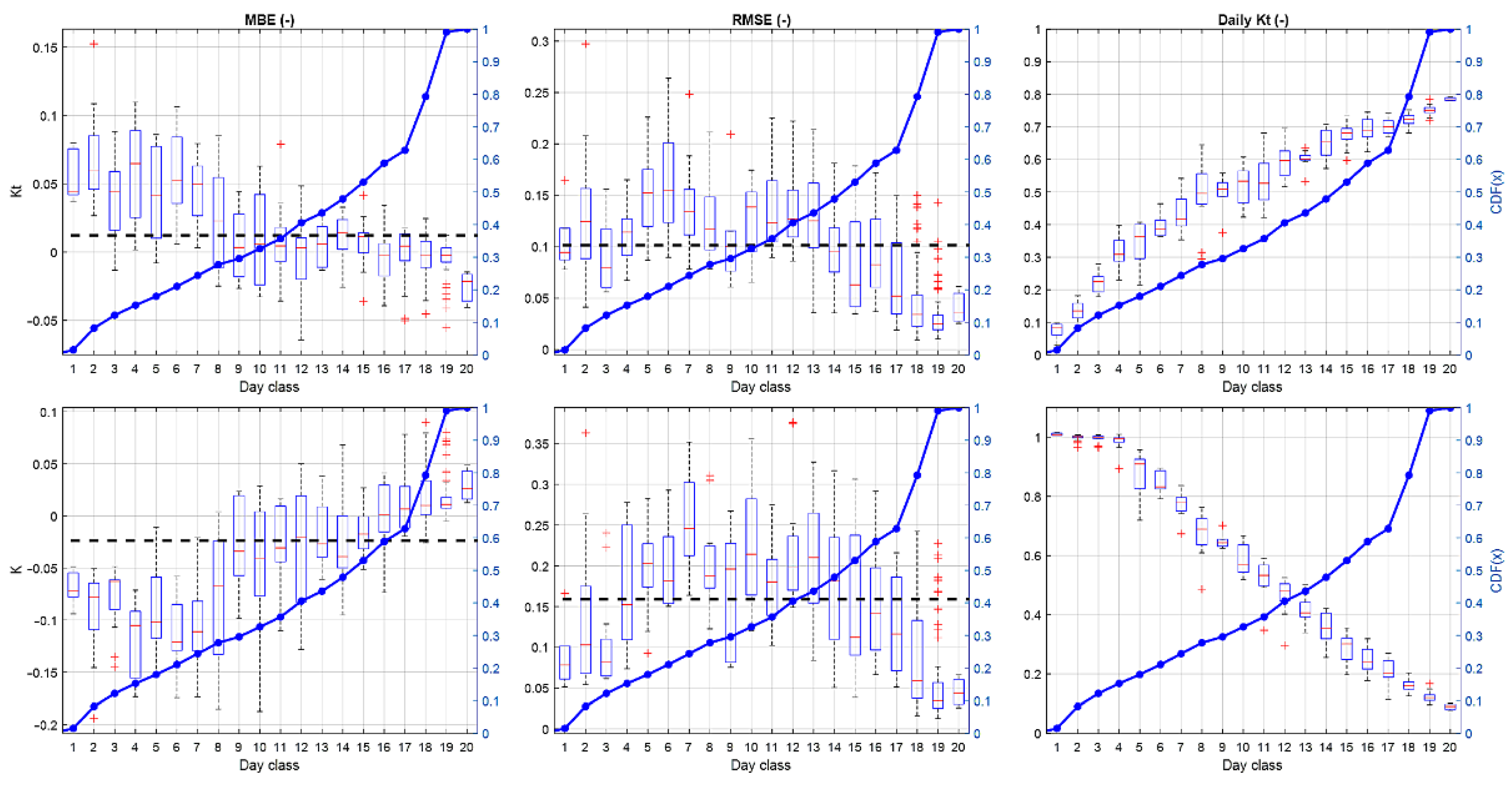
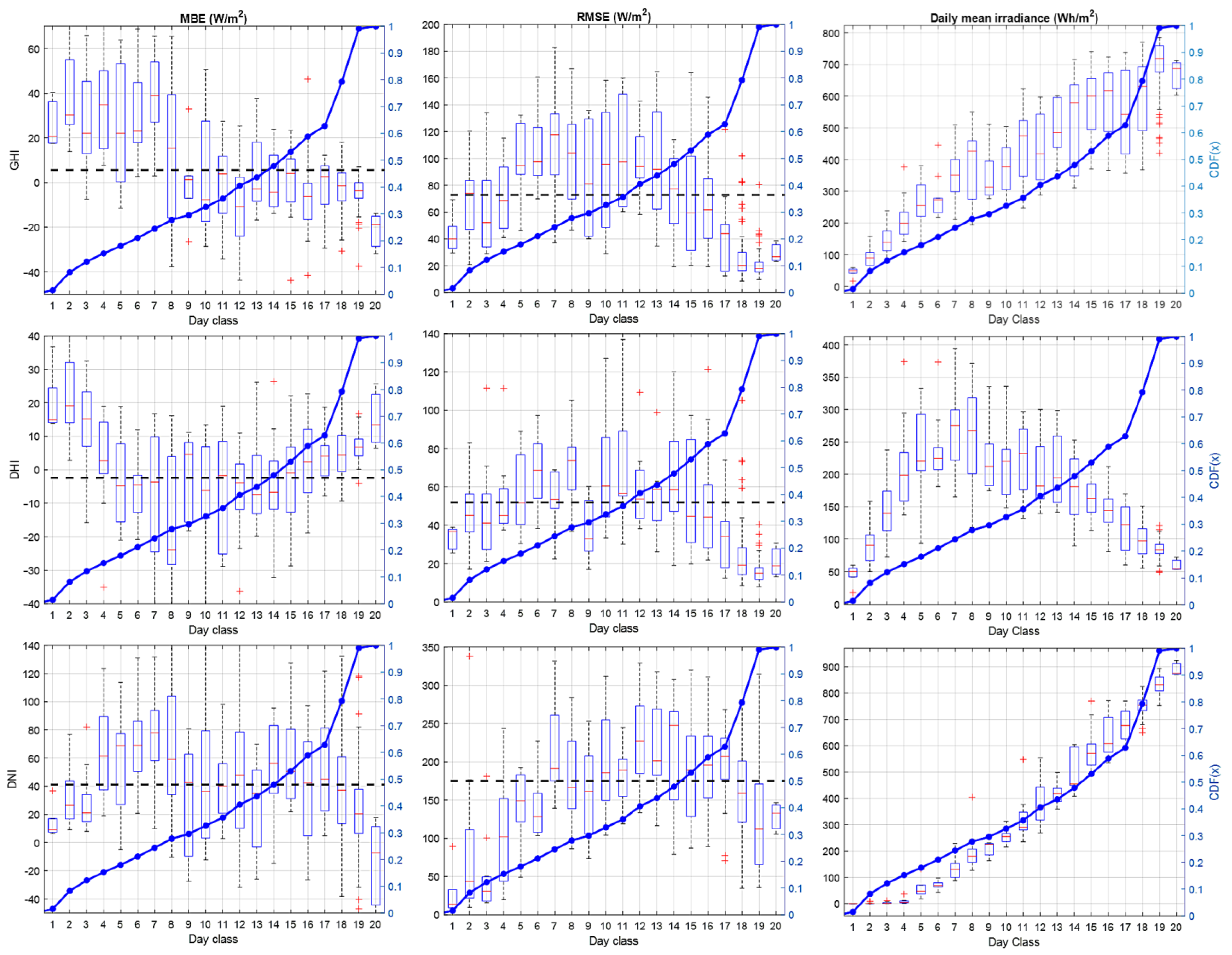
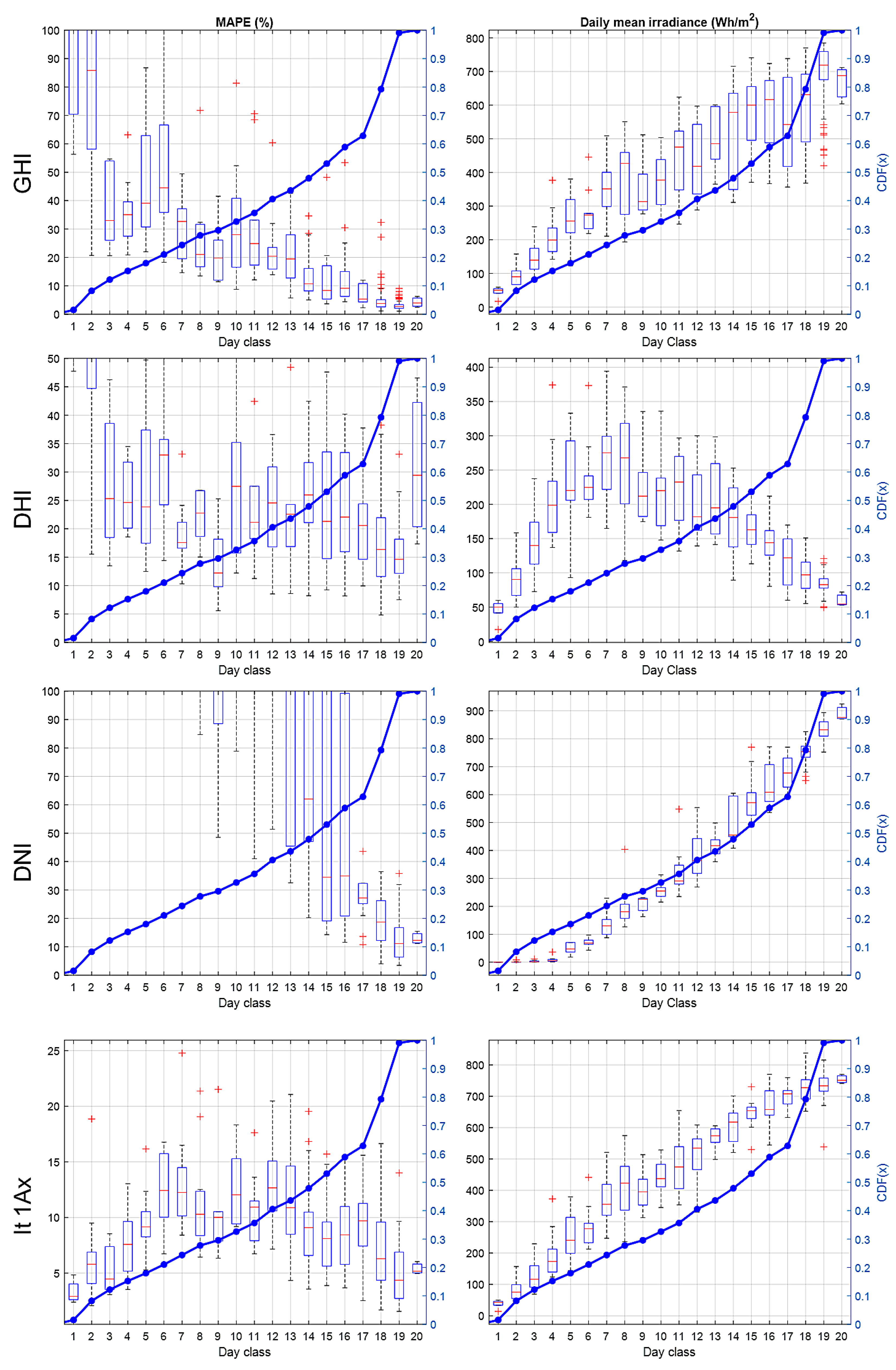
4.3. Forecast Performance Assessment as a Function of Day Type

The results presented so far corresponded to whole one-year time series of the evaluation dataset, as is often presented in literature. Nevertheless, an important aspect to analyze forecasting performance under different atmospheric conditions. While authors have previously analyzed performance according to subjective discrete day classifications [15] or as a function of specific daily K t values [14,32], the classification presented in [33] proves useful to analyze performance characteristics for deterministically defined typical day types with well-defined characteristics, independently of solar geometry and seasonal effects. Only valid data points were considered for error calculation. Figure 8 shows that when invalid days or gaps have seasonal character, this can impact the results. Performance for 2016 suddenly and significantly decreased when compared to the rest while Figure 13 shows the majority of invalid data points for this year occurred around the summer months, when the skies are clearer and the method’s performance is best.
For K t and K forecasts (Figure 14), results show poor performance for overcast conditions (day class ≤ 4), but for variable days onwards (day class ≥ 6 for K t and day class ≥ 8 for K) mean performance is consistently and significantly better than persistence, except for the clearest day class. Despite the fact that the method is clearly underperforming in a determined set of conditions, this is comparatively rare when compared to the range of meteorological conditions under analysis, as the day type distribution shows that only ~10% of days are category 4 or lower and mean day class forecasting skills are positive for over 75% of days. By recalling results for 2017 on Figure 8, the forecasting skill for K t as 0.12 while for K was 0.08; however, Figure 14 shows mean day class forecasting skills on very different ranges compared to the yearly value, which exceed it for ~60% of days for K t and K and reaching extreme values of [−0.6,0.8] and [−36,0.8], respectively. Therefore, the proposed analysis framework shows its value by allowing a deeper look into the forecasting performance for different atmospheric conditions.
Figure 15 shows similar trends for GHI and K t , with very low skill for DHI, albeit with significant spread for each day class due to the interaction between K t and K for DHI forecasting. DNI presents a significant spread at lower day classes, since DNI can be zero at overcast hours and different to zero for others, which can occur at given moments of cloudy or variable days, and this would substantially increase RMSE. However, DNI mean day class forecasting skill is consistently positive for day classes 8 onwards, which represent the vast majority of days. However, given that the proposed method’s GHI and DHI performance improves from day classes 7 onwards (≥75% of days), the forecasting skill for DNI also improves to values greater than the average 0.13 for the year. For tilted irradiances results are similar, albeit the proposed method has consistent positive skill for day classes 8 onwards (~70% of days). Due to the compounding effect of horizontally referenced irradiance forecasting and the nonlinearity of the transposition model, two observations can be made: the spread for a given day class can be significant, but the overall patterns for the different tilted planes under analysis are similar. Finally, for a finer presentation of the individual error metrics that increase the level of detail for this analysis, the reader is referred to the Appendix A.

5. Conclusions

In this work, a solar energy forecasting method was developed that estimates K t and K, the corresponding horizontally referenced irradiances on tilted, tracking surfaces. This method is based on the premise that solar irradiance patterns can be classified according to their static and dynamic characteristics through the metric termed quality score (QS) and that for any given state, there is a probability distribution function to transition to another future state. These transitions can be accurately represented by transition matrices according to solar geometry. Since each irradiance class (or state) is defined by K t , K and V S c d f , this representation proves to be independent of yearly and time-of-day seasonality, while allowing for the flexibility to capture a new location’s particular dynamics once the knowledge base is updated with fresh data for that site. Forecasting performance was assessed for 6 years in a rolling manner, for a location on which initially no data were available, to evaluate how performance changes as new local data is added to the knowledge base, simulating its operational deployment. The assessment framework is thorough, exceeding the conventional one-year assessment period of most studies and exploring not only the one-year performance, but also on a typical day case basis.
Given the marked inertias and start/stop times of hydro/thermal generators, it is necessary to provide system operators with forecast information such that it is operationally feasible to consider it in the dispatch problem to improve the solution against a no-forecast case, defining this anticipation as the forecast lead time. If this task cannot be achieved, then regardless of the forecast’s quality, it is for all practical purposes useless because it is disconnected from the application it should serve: to positively influence a decision. That is why in this work the effect of the forecast lead time in the forecast performance has been analyzed, using 0–2 h for lead time, showing that this parameter has a significant effect in forecasting performance, giving additional value to the results presented in this manuscript.
The proposed method performed competitively against other methods in the literature and consistently provided for superior performance against the reference smart persistence due to maintaining a higher correlation with the actual data time series and by being more resistant to an increase in NRMSE. The most challenging condition for the proposed method relates with changes in atmospheric conditions between sunset and sunrise that cannot be foreseen since solar data are unavailable, in which the first forecast window for a new day can exhibit significant error as it is based on the last known atmospheric state that differs greatly from the current. Nevertheless, once new data are available for the next forecast window, the method is quick to adapt and even on highly variable days it can offer superior performance compared to persistence.
A significant contribution of this study is the assessment methodology, allowing for a better understanding of the characteristics of forecasting performance in the context of the local characteristics of solar irradiance. Data availability has a definite effect in the conventional one-year assessments when data were unavailable/flawed in seasons in which the method consistently over- or under-performs the yearly mean. Additionally, for certain day types the error would consistently be much lower or higher than persistence and the overall yearly performance is determined by this distribution along with that of day types during the year, which depends upon the location. Finally, this analysis allows for identifying specific conditions where the method performed best or worst and therefore, providing information for future work concerning where improvements can be made to enhance its performance.

Author Contributions

Conceptualization, A.C.-C., J.B. and R.E.; data curation, A.C.-C.; formal analysis, A.C.-C. and J.B.; funding acquisition, R.E.; investigation, A.C.-C.; methodology, A.C.-C., J.B. and R.E.; resources, R.E.; software, A.C.-C.; supervision, J.B. and R.E.; visualization, A.C.-C.; writing—original draft, A.C.-C., J.B. and R.E.; writing—review and editing, A.C.-C., J.B. and R.E. All authors have read and agreed to the published version of the manuscript.

Funding

This work received partial financial support of the Pontificia Universidad Católica de Chile by means of a VRI-CPD doctoral scholarship and partial financial support from CORFO project 13CEI2-21803. The APC was funded by own research funds from Pontificia Universidad Católica de Chile.

Acknowledgments

Armando Castillejo-Cuberos wishes to acknowledge financial support for this work from the VRI-CPD Scholarship granted by the Pontificia Universidad Católica de Chile.

Conflicts of Interest

The authors declare no conflict of interest. Additionally, the funders had no role in the design of the study; in the collection, analyses, or interpretation of data; in the writing of the manuscript, or in the decision to publish the results.

Appendix A

This Appendix presents in a finer detail the individual error metrics for the assessed forecast method, to supplement the results shown in Section 4.3 of the manuscript. Namely, MBE, RMSE and MAPE are presented for each day class, along with the corresponding distributions of K t , K and irradiance.
Figure A1 presents MBE and RMSE for K t and K, along with the corresponding range of daily values, to further contextualize the characteristics of each day type. The proposed method shows a marked bias to forecast clearer conditions for day classes under 6, which explains the comparatively poor performance under these conditions (daily K t < 0.3 and K > 0.8). As expected, RMSE tends to increase for the middle day classes, due to the fact that these are the ones that present the greatest variability.
Figure A1. Error metrics for K t   (top row) and K (bottom row) as a function of day class. Dashed line represents yearly performance. Cumulative distribution of day types presented in secondary axis.
Energies 14 06005 g0a1
Figure A2 presents a similar analysis, but for GHI, DHI, DNI and one-axis tracking tilted irradiance, while Figure A3 presents the MAPE. GHI exhibits the same MBE and RMSE patterns as K t , as expected, but with a wider spread of values for each class, due to the different I o that could occur on each day. DHI can have significant percent errors for the more overcast day classes but otherwise is 15–35% for the remainder. As presented in Section 4.3, DNI has the highest MAPE and RMSE error at lower day classes due to estimation of DNI by the forecaster in instances when there is none, even if the MBE is comparatively low. Finally, tilted irradiance exhibits a consistently low mean bias across day classes, with RMSE under 25% in the worst conditions, with similar MAPE values, although for the vast majority of days (and the yearly mean) it is close to 10%. Results for tilted irradiance are presented for one-axis tracking only due to similarity to other tracking planes, as to avoid redundancy.
Figure A2. Error metrics for GHI (top row), DHI (middle row) and DNI (bottom row) as a function of day class. Dashed line represents yearly performance. Cumulative distribution of day types presented in secondary axis.
Energies 14 06005 g0a2
Figure A3. MAPE for irradiance forecasting as a function of day class. Cumulative distribution of day types presented in secondary axis.
Energies 14 06005 g0a3

References

  1. Denholm, P.; Mai, T. Timescales of Energy Storage Needed for Reducing Renewable Energy Curtailment Timescales of Energy Storage Needed for Reducing Renewable Energy Curtailment; National Renewable Energy Laboratory (NREL): Golden, CO, USA, 2017.
  2. Denholm, P.; Margolis, R. The Potential for Energy Storage to Provide Peaking Capacity in California under Increased Penetration of Solar Photovoltaics; National Renewable Energy Laboratory (NREL): Golden, CO, USA, 2018.
  3. Diagne, M.; David, M.; Lauret, P.; Boland, J.; Schmutz, N. Review of solar irradiance forecasting methods and a proposition for small-scale insular grids. Renew. Sustain. Energy Rev. 2013, 27, 65–76. [Google Scholar] [CrossRef] [Green Version]
  4. Antonanzas, J.; Osorio, N.; Escobar, R.; Urraca, R.; Martinez-de-Pison, F.J.; Antonanzas-Torres, F. Review of photovoltaic power forecasting. Sol. Energy 2016, 136, 78–111. [Google Scholar] [CrossRef]
  5. Voyant, C.; Notton, G.; Kalogirou, S.; Nivet, M.-L.; Paoli, C.; Motte, F.; Fouilloy, A. Machine learning methods for solar radiation forecasting: A review. Renew. Energy 2017, 105, 569–582. [Google Scholar] [CrossRef]
  6. Sobri, S.; Koohi-Kamali, S.; Rahim, N.A. Solar photovoltaic generation forecasting methods: A review. Energy Convers. Manag. 2018, 156, 459–497. [Google Scholar] [CrossRef]
  7. Yang, D.; Kleissl, J.; Gueymard, C.A.; Pedro, H.T.C.; Coimbra, C.F.M. History and trends in solar irradiance and PV power forecasting: A preliminary assessment and review using text mining. Sol. Energy 2018, 168, 60–101. [Google Scholar] [CrossRef]
  8. Guermoui, M.; Melgani, F.; Gairaa, K.; Mekhalfi, M.L. A comprehensive review of hybrid models for solar radiation forecasting. J. Clean. Prod. 2020, 258, 120357. [Google Scholar] [CrossRef]
  9. Ljung, L. Identification: Theory for the User; Prentice Hall: Hoboken, NJ, USA, 1987. [Google Scholar]
  10. Box, G.E.P.; Jenkins, G.M.; Day, H. Time Series Analysis: Forecasting and Control; Holden-Day: San Francisco, CA, USA, 1976; ISBN 9780816211043. [Google Scholar]
  11. Alkhayat, G.; Mehmood, R. A Review and Taxonomy of Wind and Solar Energy Forecasting Methods Based on Deep Learning. Energy AI 2021, 4, 100060. [Google Scholar] [CrossRef]
  12. Cai, M.; Pipattanasomporn, M.; Rahman, S. Day-ahead building-level load forecasts using deep learning vs. traditional time-series techniques. Appl. Energy 2019, 236, 1078–1088. [Google Scholar] [CrossRef]
  13. Lan, H.; Zhang, C.; Hong, Y.Y.; He, Y.; Wen, S. Day-ahead spatiotemporal solar irradiation forecasting using frequency-based hybrid principal component analysis and neural network. Appl. Energy 2019, 247, 389–402. [Google Scholar] [CrossRef]
  14. Theocharides, S.; Makrides, G.; Livera, A.; Theristis, M.; Kaimakis, P.; Georghiou, G.E. Day-ahead photovoltaic power production forecasting methodology based on machine learning and statistical post-processing. Appl. Energy 2020, 268, 115023. [Google Scholar] [CrossRef]
  15. Du Plessis, A.A.; Strauss, J.M.; Rix, A.J. Short-term solar power forecasting: Investigating the ability of deep learning models to capture low-level utility-scale Photovoltaic system behaviour. Appl. Energy 2021, 285, 116395. [Google Scholar] [CrossRef]
  16. Wang, H.; Cai, R.; Zhou, B.; Aziz, S.; Qin, B.; Voropai, N.; Gan, L.; Barakhtenko, E. Solar irradiance forecasting based on direct explainable neural network. Energy Convers. Manag. 2020, 226, 113487. [Google Scholar] [CrossRef]
  17. Sethi, T.S.; Kantardzic, M. Data driven exploratory attacks on black box classifiers in adversarial domains. Neurocomputing 2018, 289, 129–143. [Google Scholar] [CrossRef] [Green Version]
  18. Wang, F.; Xuan, Z.; Zhen, Z.; Li, K.; Wang, T.; Shi, M. A day-ahead PV power forecasting method based on LSTM-RNN model and time correlation modification under partial daily pattern prediction framework. Energy Convers. Manag. 2020, 212, 112766. [Google Scholar] [CrossRef]
  19. Ahmed, R.; Sreeram, V.; Mishra, Y.; Arif, M.D. A review and evaluation of the state-of-the-art in PV solar power forecasting: Techniques and optimization. Renew. Sustain. Energy Rev. 2020, 124, 109792. [Google Scholar] [CrossRef]
  20. Wang, F.; Zhang, Z.; Liu, C.; Yu, Y.; Pang, S.; Duić, N.; Shafie-khah, M.; Catalão, J.P.S. Generative adversarial networks and convolutional neural networks based weather classification model for day ahead short-term photovoltaic power forecasting. Energy Convers. Manag. 2019, 181, 443–462. [Google Scholar] [CrossRef]
  21. Yang, D.; Alessandrini, S.; Antonanzas, J.; Antonanzas-Torres, F.; Badescu, V.; Beyer, H.G.; Blaga, R.; Boland, J.; Bright, J.M.; Coimbra, C.F.M.; et al. Verification of deterministic solar forecasts. Sol. Energy 2020, 210, 20–37. [Google Scholar] [CrossRef]
  22. Yang, D. Making reference solar forecasts with climatology, persistence, and their optimal convex combination. Sol. Energy 2019, 193, 981–985. [Google Scholar] [CrossRef]
  23. Paulescu, M.; Paulescu, E.; Badescu, V. Nowcasting solar irradiance for effective solar power plants operation and smart grid management. In Predictive Modelling for Energy Management and Power Systems Engineering; Elsevier: Amsterdam, The Netherlands, 2021; pp. 249–270. [Google Scholar]
  24. Coimbra, C.F.M.; Pedro, H.T.C. Stochastic-Learning Methods. In Solar Energy Forecasting and Resource Assessment; Elsevier: Amsterdam, The Netherlands, 2013; pp. 383–406. [Google Scholar]
  25. Notton, G.; Voyant, C. Forecasting of Intermittent Solar Energy Resource. In Advances in Renewable Energies and Power Technologies; Elsevier: Amsterdam, The Netherlands, 2018; pp. 77–114. [Google Scholar]
  26. Rodríguez-Benítez, F.J.; Arbizu-Barrena, C.; Huertas-Tato, J.; Aler-Mur, R.; Galván-León, I.; Pozo-Vázquez, D. A short-term solar radiation forecasting system for the Iberian Peninsula. Part 1: Models description and performance assessment. Sol. Energy 2020, 195, 396–412. [Google Scholar] [CrossRef]
  27. Aguiar, L.M.; Pereira, B.; Lauret, P.; Díaz, F.; David, M. Combining solar irradiance measurements, satellite-derived data and a numerical weather prediction model to improve intra-day solar forecasting. Renew. Energy 2016, 97, 599–610. [Google Scholar] [CrossRef] [Green Version]
  28. Fouilloy, A.; Voyant, C.; Notton, G.; Duchaud, J.-L. Regression trees and solar radiation forecasting: The boosting, bagging and ensemble learning cases. In Proceedings of the 2nd International Web Conference on Forecasting, Online, 15–17 October 2018. [Google Scholar]
  29. Heydari, A.; Astiaso Garcia, D.; Keynia, F.; Bisegna, F.; De Santoli, L. A novel composite neural network based method for wind and solar power forecasting in microgrids. Appl. Energy 2019, 251, 113353. [Google Scholar] [CrossRef]
  30. Kumari, P.; Toshniwal, D. Extreme gradient boosting and deep neural network based ensemble learning approach to forecast hourly solar irradiance. J. Clean. Prod. 2021, 279, 123285. [Google Scholar] [CrossRef]
  31. Rafati, A.; Joorabian, M.; Mashhour, E.; Shaker, H.R. High dimensional very short-term solar power forecasting based on a data-driven heuristic method. Energy 2021, 219, 119647. [Google Scholar] [CrossRef]
  32. Betti, A.; Pierro, M.; Cornaro, C.; Moser, D.; Moschella, M.; Collino, E.; Ronzio, D.; van der Meer, D.; Visser, L.; Widen, J.; et al. Regional Solar Power Forecasting 2020; IEA-PVPS: Paris, France, 2020. [Google Scholar]
  33. Castillejo-Cuberos, A.; Escobar, R. Understanding solar resource variability: An in-depth analysis, using Chile as a case of study. Renew. Sustain. Energy Rev. 2020, 120, 109664. [Google Scholar] [CrossRef]
  34. Yang, D.; Wu, E.; Kleissl, J. Operational solar forecasting for the real-time market. Int. J. Forecast. 2019, 35, 1499–1519. [Google Scholar] [CrossRef]
  35. Castillejo-Cuberos, A.; Escobar, R. Detection and characterization of cloud enhancement events for solar irradiance using a model-independent, statistically-driven approach. Sol. Energy 2020, 209, 547–567. [Google Scholar] [CrossRef]
  36. Rigollier, C.; Bauer, O.; Wald, L. On the clear sky model of the ESRA—European Solar Radiation Atlas—With respect to the heliosat method. Sol. Energy 2000, 68, 33–48. [Google Scholar] [CrossRef] [Green Version]
  37. Ghimire, S.; Deo, R.C.; Raj, N.; Mi, J. Deep solar radiation forecasting with convolutional neural network and long short-term memory network algorithms. Appl. Energy 2019, 253, 113541. [Google Scholar] [CrossRef]
  38. Bhardwaj, S.; Sharma, V.; Srivastava, S.; Sastry, O.S.; Bandyopadhyay, B.; Chandel, S.S.; Gupta, J.R.P. Estimation of solar radiation using a combination of Hidden Markov Model and generalized Fuzzy model. Sol. Energy 2013, 93, 43–54. [Google Scholar] [CrossRef]
  39. Sanjari, M.J.; Gooi, H.B. Probabilistic Forecast of PV Power Generation Based on Higher Order Markov Chain. IEEE Trans. Power Syst. 2017, 32, 2942–2952. [Google Scholar] [CrossRef]
  40. Lave, M.; Reno, M.J.; Broderick, R.J. Characterizing local high-frequency solar variability and its impact to distribution studies. Sol. Energy 2015, 118, 327–337. [Google Scholar] [CrossRef]
  41. Zadeh, L.A. Fuzzy sets. Inf. Control 1965, 8, 338–353. [Google Scholar] [CrossRef] [Green Version]
  42. Zadeh, L.A. Discussion: Probability Theory and Fuzzy Logic Are Complementary Rather Than Competitive. Technometrics 1995, 37, 271–276. [Google Scholar] [CrossRef]
  43. Zadeh, L.A. Fuzzy sets as a basis for a theory of possibility. Fuzzy Sets Syst. 1999, 100, 9–34. [Google Scholar] [CrossRef]
  44. Kovalerchuk, B. Relationships Between Probability and Possibility Theories. In Uncertainty Modeling; Springer: Cham, Switzerland, 2017; Volume 683, pp. 97–122. ISBN 9783319510514. [Google Scholar]
  45. Natvig, B. Possibility versus probability. Fuzzy Sets Syst. 1983, 10, 31–36. [Google Scholar] [CrossRef]
  46. Barragán, A. Síntesis de Sistemas de Control Borroso Estables por Diseño. Ph.D. Thesis, Universidad de Huelva, Huelva, Spain, 2009. [Google Scholar]
  47. Long, C.; Shi, Y. The QCRad Value Added Product: Surface Radiation Measurement Quality Control Testing, Including Climatology Configurable Limits; U.S. Department of Energy, Office of Science Atmospheric Radiation Measurement Program: Washington, DC, USA, 2006.
  48. Journée, M.; Bertrand, C. Quality control of solar radiation data within the RMIB solar measurements network. Sol. Energy 2011, 85, 72–86. [Google Scholar] [CrossRef]
  49. Duffie, J.A.; Beckman, W.A. Solar Engineering of Thermal Processes; Wiley: New York, NY, USA, 2013. [Google Scholar]
  50. Antonanzas-Torres, F.; Urraca, R.; Polo, J.; Perpiñán-Lamigueiro, O.; Escobar, R. Clear sky solar irradiance models: A review of seventy models. Renew. Sustain. Energy Rev. 2019, 107, 374–387. [Google Scholar] [CrossRef]
  51. Polo, J.; Antonanzas-Torres, F.; Vindel, J.M.; Ramirez, L. Sensitivity of satellite-based methods for deriving solar radiation to different choice of aerosol input and models. Renew. Energy 2014, 68, 785–792. [Google Scholar] [CrossRef]
  52. Beyer, H.; Martinez, J.P.; Suri, M.; Torres, J.; Lorenz, E.; Müller, S.; Hoyer-Klick, C.; Ineichen, P. Report on Benchmarking of Radiation Products; Management and Exploitation of Solar Resource Knowledge (MESOR): Cologne, Germany, 2009. [Google Scholar]
  53. Taylor, K.E. Summarizing multiple aspects of model performance in a single diagram. J. Geophys. Res. Atmos. 2001, 106, 7183–7192. [Google Scholar] [CrossRef]
Figure 1. Some selected results from the literature showcasing typical performance cases for solar radiation forecasting, based on [27,28].
Energies 14 06005 g001
Figure 2. Application of Box–Jenkins methodology to different irradiance patterns from overcast to clear sky. One-minute clear sky irradiance hourly patterns (top left), with most representative time series of each set (top right). Lower subfigures present autocorrelation (bottom left) and partial autocorrelation functions (bottom right) for each representative time series. Color bar in top-left subfigure represents probability of occurrence.
Energies 14 06005 g002
Figure 3. Typical one-minute clear sky clearness index time series for a representative hour for each irradiance class, with its corresponding K t and K value ranges, based on [33].
Energies 14 06005 g003
Figure 4. Workflow to construct transition probability matrixes after irradiance pattern classification has been performed.
Energies 14 06005 g004
Figure 5. Summary of fuzzy inference system workflow.
Energies 14 06005 g005
Figure 6. Workflow to determine the likelihood function for QS on a test case with origin state: K t = 0.667, K = 0.333 and QS = 0.667. Membership function for QS (a), state transition probability matrix (b), future state probability of occurrence (c), QS ranges for each destination state (d), probability-weighed likelihood function for QS at each possible destination state (e), likelihood function for QS (f).
Energies 14 06005 g006
Figure 7. Workflow for the inference and de-fuzzification stages. Case with origin state: K t = 0.667, K = 0.333 and QS = 0.667. QS in the Kt-K space at the likely V S c d f value (a), QS likelihood function (b), QS likelihood mapped to the Kt-K space (c), plausibility space (d), combined Kt-K likelihood (e), overall likelihood function for a Kt-K-QS triad, with the forecasted value at the centroid (f).
Energies 14 06005 g007
Figure 8. Effect of data aggregation to the knowledge base on forecasting skill.
Energies 14 06005 g008
Figure 9. Example forecasting time series for the proposed method, showcasing completely clear (first), clear (second) and highly variable (third) days in the Santiago 2017 dataset: clearness index and diffuse fraction (a), horizontally referenced irradiance (b) and tilted plane irradiance (c).
Energies 14 06005 g009
Figure 10. Forecasting skill performance for different forecast horizons and lead times (FLT), time units in hours: clearness index and diffuse fraction in the first row, horizontally referenced irradiance middle row and tilted plane irradiance bottom row.
Energies 14 06005 g010
Figure 11. Taylor diagrams for Kt (left) and K (right) forecasting. Hours in the chart indicate forecast horizon. Standard deviation and RMSD are in percent.
Energies 14 06005 g011
Figure 12. Taylor diagrams for irradiance forecasting. Hours in chart indicate forecast horizon, standard deviation and RMSD are in percent for tilted irradiance and in W/m2 for horizontally referenced irradiance. Mean GHI = 502.62 W/m2 Mean DNI = 503.74 W/m2 and Mean DHI = 148.35 W/m2.
Energies 14 06005 g012
Figure 13. Valid (yellow) and invalid (blue) days for each available year of data for Santiago.
Energies 14 06005 g013
Figure 14. Skill score distributions for K t and K as a function of day class. Dashed line represents yearly performance. Cumulative distribution of day types presented in secondary axis.
Energies 14 06005 g014
Figure 15. Skill score distributions for irradiance as a function of day class. Dashed line represents yearly performance. Cumulative distribution of day types presented in secondary axis.
Energies 14 06005 g015
Table 1. Example artificial intelligence approaches for solar radiation forecasting.
SourceMethodDataset
Lan et al. [13] Combination of frequency analysis to identify irradiance patterns, principal component analysis to identify characteristic features and neural networks are used to forecast future features of irradiance that are translated back to an irradiance forecast.One year of data
Theocharides et al. [14]Several neural networks were developed to produce GHI forecasts, which are then clusterized and finally, through statistical processing, the final forecast is produced as a linear combination of the clusters.210 days
Du Plessis et al. [15]Several neural networks were developed for meteorological data to forecast a photovoltaic plant output at the subunit level and then scaled up to plant-wide production.Two years training and 1 year of validation data.
Table 2. Current issues in artificial intelligence applications for solar power forecasting.
SourceIssue or Concern
Wang et al. [16] and Sethi and Kantardzic [17]Neural networks/deep learning approaches have not seen sufficient adoption, despite growing interest in them, due to their complex black-box nature and lack of explainability and interpretability
Wang. et al. [18]These approaches are prone to model overfitting and insufficient generalization ability, being hyperspecific.
Wang. et al. [16] Explainability is of great importance, therefore, proposed a new approach through direct explainable neural networks that can provide further insights in the input–output relationship to assist in result interpretation and model explanation.
Ahmed et al. [19]Appropriate weather classification is important for solar photovoltaic power forecasting assessment, and there are challenges to overcome in these classifications, presenting that most authors employ four or less classes.
Wang et al. [20]Separate forecast models for each weather class should improve forecasting performance; therefore, having a higher number of classes would be beneficial.
Publisher’s Note: MDPI stays neutral with regard to jurisdictional claims in published maps and institutional affiliations.

