Article

Machine Learning and Data Segmentation for Building Energy Use Prediction—A Comparative Study

School of Computing, Engineering and Digital Technology (SCEDT), Teesside University, Middlesbrough TS1 3BA, UK
*
Author to whom correspondence should be addressed.
Energies 2021, 14(18), 5947; https://doi.org/10.3390/en14185947
Submission received: 17 June 2021 / Revised: 4 August 2021 / Accepted: 12 September 2021 / Published: 18 September 2021
(This article belongs to the Topic Power System Modeling and Control)

Abstract

:
Advances in metering technologies and emerging energy forecast strategies provide opportunities and challenges for predicting both short and long-term building energy usage. Machine learning is an important energy prediction technique, and is significantly gaining research attention. The use of different machine learning techniques based on a rolling-horizon framework can help to reduce the prediction error over time. Due to the significant increases in error beyond short-term energy forecasts, most reported energy forecasts based on statistical and machine learning techniques are within the range of one week. The aim of this study was to investigate how facility managers can improve the accuracy of their building’s long-term energy forecasts. This paper presents an extensive study of machine learning and data processing techniques and how they can more accurately predict within different forecast ranges. The Clarendon building of Teesside University was selected as a case study to demonstrate the prediction of overall energy usage with different machine learning techniques such as polynomial regression (PR), support vector regression (SVR) and artificial neural networks (ANNs). This study further examined how preprocessing training data for prediction models can impact the overall accuracy, such as via segmenting the training data by building modes (active and dormant), or by days of the week (weekdays and weekends). The results presented in this paper illustrate a significant reduction in the mean absolute percentage error (MAPE) for segmented building (weekday and weekend) energy usage prediction when compared to unsegmented monthly predictions. A reduction in MAPE of 5.27%, 11.45%, and 12.03% was achieved with PR, SVR and ANN, respectively.

1. Introduction

Building energy use prediction models can either be produced during a building’s design, calibration, or occupancy period, to assist in the creation of optimised building and management plans for the reduction in building energy usage. Whereas design stage models tend towards using either physics engines, statistical models or historical data from other sites, calibration and occupancy period models have the advantage of being able to use data from the actual building site to enhance their building energy use predictions. An issue that can occur with energy use prediction models is that the accuracy can deteriorate over time due to changes in overall energy usage. As a building ages, its physical properties change, as does the usage of the building by the building occupants. These changes may be beneficial, for example, in the cases of renovations to improve overall building energy efficiency, or negative, for example, in the case of materials decaying over time. Whether the change is beneficial or negative, the result is that if a building’s prediction model is not retrained or remade with up-to-date data, the ability to accurately predict the energy use will decrease. This can lead to a reduced ability of a facility manager to effectively predict their building energy usage and enact energy plans and policies appropriately due to their ability to incorporate and map the large (often up to date) datasets typically associated with building management systems. Machine learning (ML) techniques tend towards being more accurate than physics models for predicting building energy use “when training data is abundant”. Machine learning techniques are, however, less generalist and predict less accurately when extrapolating outside of available training data [1]. In recent years, there has been increased interest in using machine learning for predicting building energy usage during the occupancy stage in academic research, with multiple direct comparisons of the ability of the machine learning technique to predict building energy usage using the same datasets. It is considerably rarer, however, when multiple machine learning techniques are compared over multiple ranges [2,3,4,5,6]. Comparisons involving multiple ranges of building energy forecasts usually occur only when testing a singular learning technique. Although the accuracy of machine learning techniques can be compared and evaluated when tested on a single dataset, the observed error is of limited value for comparative purposes with machine learning techniques trained upon different datasets, such as those of different time periods, sites or sources. This limits the ability to compare the impact of using different machine learning techniques across multiple case studies, as it is not known how the machine learning techniques would have performed with the use of alternative datasets.
This study focused on the impact of using different machine learning techniques, as the forecast range increases, on the accuracy of said building level energy use predictions. This was to investigate if the error of long-term predictions (monthly) can be reduced through data segmentation to or below the level of the average error in short-term predictions (daily and weekly). This study was performed as part of a greater research project investigating the impact of using different machine learning techniques on the accuracy of predicting building energy usage over a rolling horizon framework, and how forecasting error can be reduced using data segmentation. An example of the latter is the examination of whether it would be more accurate to model each energy meter in a building and sum their predictions, or only model the net building energy usage. Data segmentation is the process of dividing and grouping datasets based on pre-chosen parameters, which, in the case of this study, were timeframes (i.e., building active and dormancy periods, and weekday and weekend energy use). This is done so that the datasets can be used more effectively to create two distinct prediction models for the separate groups of data, which, in theory, would predict the segments more accurately than a model trained on both. It was assumed by the authors of this paper that it would be possible to improve the accuracy of building level energy use predictions via data segmentation and the creation of multiple predictive models, compared to a singular model, via better accommodation of the different building energy use behaviours that occur in the Clarendon building. It is envisioned that, by improving the ability of facility managers to predict their building’s energy use, they may be able to implement building energy management policies and programs, such as building demanded response systems, more effectively. The increased effectiveness of their ability to predict their building energy use can contribute to a reduction in the increase in building energy usage across the developed and developing world [7]. Data segmentation has been used historically in marketing to better predict the success of marketing to different groups, by developing different models for potential customers based on their demographics, lifestyles, behaviours, and value (as a customer) [8]. First defined in 1956, market segmentation is one of the most widely accepted and increasingly important concepts in academic research into marketing and predicting consumer needs [9,10].
The impact of attempts to make use of data segmentation to improve the accuracy of building energy prediction models have been mixed. In comparison to predictions based on control data, the average accuracy of building energy use forecasts was reduced by 80% via the removal of outliners in the training data in one case study [11]. Within the scope of the energy use of event venues, however, it was identified that the difference in energy use between event and non-event days in an unsegmented model was unable to accurately accommodate both on- and off-event days. This issue was resolved through the creation of separate models for on- and off-event days, which allowed for accurate predictions of both periods to occur separately [12]. There is the potential to either increase or decrease the accuracy of building energy forecasts dependent upon how the datasets are segmented. To test the potential of data segmentation to improve predictions, methods of modelling and predicting building energy use were selected after reviewing the literature published within the last five years on predicting building energy usage. The most used ML techniques in the field of forecasting building energy use were: artificial neural networks (ANNs), support vector machines (SVMs), distribution regression, and clustering [13]. Due to their capacity to interpret nonlinear data in irregular energy usage environments, ANNs and SVR were selected for use for modelling within this study. SVRs generally possess greater accuracy when only smaller datasets are available than ANNs, but are outperformed by ANNs when larger datasets are available [12]. Additionally, PR is used as a comparative tool with ANN and SVR, due to its ease and speed of use. Although hybrid models often outperform monotype models, the hybridisation often increases the complexity of use of such models, requiring additional skills to use these more advanced systems. It cannot be assumed that facility managers that may wish to improve the long-term building energy predictions will have familiarity with advanced machine learning techniques. Hybrid models are ignored in this study in favour of easier-to-use predictive systems.
This paper considers the predictive forecasting of net building energy use, using a case study of the Clarendon building at Teesside University Campus in the UK, to demonstrate overall building energy forecasts over a range of three time intervals: daily, weekly, and monthly for each season of 2018. Due to its data rich environment provided by its Building Management System (BMS), the Clarendon building of Teesside University was selected for use in this study. Previous studies of this building utilising regression squared analysis typically had a baseline of 20% mean absolute prediction error (MAPE) for the demands of each asset in day-ahead forecasts [14]. To test the impact of data segmentation, in this study the Clarendon building’s energy use was forecasted using multiple machine learning techniques (PR, SVR and ANN). The data was divided into three groups: a control group, a group that was segmented into weekdays and weekends, and a group that was segmented into building active and building dormancy periods. Each of the variables was tested over the three time intervals of each season. It was initially hypothesised in this experiment that: (i) as the forecast range increases, the accuracy of all of the learning techniques will decrease and, although SVR would perform more accurately for the short-term daily predictions, ANN would perform more accurately in the long-term monthly predictions; (ii) that summer and winter would, on average, have higher accuracy in their predictions than autumn or spring, as they would require more regular heating ventilation and air conditioning (HVAC) usage, which in theory should be easier to identify and predict, than the expected erratic use in spring and autumn; and (iii) by segmenting the prediction models to accommodate for the different energy use patterns that occur during the day and week, the net accuracy of these models’ predictions would both be higher than the unsegmented models’ predictions the same period.
The remainder of this paper is structured as follows: Section 2 presents a review of related work and highlights the contribution of the current paper. Section 3 describes the research methods used, and Section 4 describes how the models used in the research method were calibrated. Section 5 describes the impact of data segmentation on the three models used to predict building energy usage over multiple forecast ranges. Section 6 concludes the paper and outlines areas for future work.

2. State of the Art

It was predicted by the Organisation for Economic Cooperation and Development (OECD), that for member nations, including Australia, New Zealand, United Kingdom, and United States of America, energy consumption by buildings (commercial and residential) would grow from 2012 to 2040, on average, by 1.5% per year. Non-OECD nations, predominately developing nations, have a predicted 2.1% growth per year of building energy consumption over the same period [7]. To reduce this trend, of which many approaches have and are being attempted, the development of increasingly efficient building systems is essential [15]. With regards to reducing the energy consumption of smart buildings, precise predictions for building energy consumption loads have the potential to confer significant benefits. These allow for accurate demand response strategies for peak load reduction, reducing electricity use and integrating distributed energy resources [16]. Although numerous software systems have been developed for designing and estimating the energy efficiency and consumption of new buildings (e.g., EnergyPlus, eQUEST, BLAST, and DeST), it is difficult to predict future building energy usage because the building energy behaviour is influenced by multiple independent factors [17]. A building’s energy consumption is influenced by its thermal properties (construction materials, window size, and material shape and volume), lighting, heating, cooling, air ventilation, and the occupants’ electricity demands [17,18]. Whereas buildings thermal properties are fixed (subject to deterioration over time), the remaining influential factors are not, and are subject to the occupants’ schedules and local weather conditions [18]. Due to these factors, it is difficult to make accurate building energy consumption predictions with a forecast horizon of greater than one hour. This is also due to the massive amount of data that must be processed for this prediction to occur. These predictions are often not useful due to the error that can occur in the prediction beyond a one-hour range [19]. To address this issue, many forms of machine learning have been used historically, with an increasing trend towards hybridisation to accommodate the inherent strengths and weakness of the machine learning techniques [15,20,21,22,23]. Hybridisation increases the accuracy of the predictions, at the cost of increased model complexity and skill requirements.
The recent and significant increase in research related to the forecasting of energy consumption of buildings is facilitated by and partially due to the increasing number of buildings that are equipped with smart meters that gather related load data at sub-hourly granularities [16]. In this study, an alternative approach to hybridisation was taken, investigating the potential for enhancing smart meter data and its structure, to improve model accuracy, rather than attempting to directly improve the structure of the machine learning techniques. This was part of a greater push to improve the data available for use in models, rather than the models themselves [24]. The impact of different types of data input on predicting building energy use has been analysed by numerous researchers. Indoor occupancy of the building plays a major, precarious, and demanding role in energy prediction modelling for buildings [25]. One approach to improve the accuracy of the modelling prediction can be accomplished through the integration of a clear and fixed occupancy schedule, based on fixed time ranges, in terms of either hours or weekdays and weekends, as an input to the building energy model. Rather than inputting the expected occupancy, which is difficult to predict in a university complex, or a specification of the occupancy period (weekdays and weekends), this study examined the creation of entirely separate models for predicting each occupancy period. In theory, this should allow each model to more easily identify, and then adapt to, the variances inherent in building energy consumption caused by occupancy, of which the most pronounced variations exist between weekdays and weekends, and workhours and non-work hours [26].
To identify the scope for improvement and realise the potential of machine learning techniques, a review of the current and previous research projects within the past five years (2016 to 2021), using the most used machine learning techniques (ANN, SVR and multiple linear regression (MLR)) [27] for predicting building energy use was conducted [2,3,5,7,15,16,17,18,19,20,21,22,23,24,25,26,27,28,29,30,31,32,33,34,35,36,37,38,39,40,41,42,43,44,45,46,47,48,49,50,51,52,53,54,55,56,57,58,59,60,61,62,63,64,65,66,67,68,69,70,71,72,73,74]. Although an objective of this review was to identify twenty-five papers corresponding to each learning technique, due to the overlap of comparative papers containing multiple machine learning techniques, which thus appeared in separate systematic searches, only sixty-five rather than seventy-five papers were reviewed. The percentages in Section 2.1, Section 2.2 and Section 2.3 refer to the number of papers that correlate with the statements before them. From this process, it was identified that building energy consumption prediction has historically been categorised into four main groups based upon their forecast horizon: very short forecasts from a minute to an hour; short-term for forecasts from one day to one week ahead; medium-term for forecasts for two weeks to multiple months ahead; and long-term for load forecasts from a few months to years [16]. However, in this study, they were defined as very short (predictions up to an hour), short (predictions above an hour, up to a day), medium (predictions above a day, up to a week), long (predictions above a week, up to a month) and very long (for any predictions longer than a month). These definitions were chosen because they offer a better description for studies in which forecast ranges fall between the previous definitions.
In a previous paper by Mounter et al. (2020), investigations into the impact of data segmentation on extreme learning machine (ELM) predictions using Clarendon building HVAC data were carried out. The obtained results indicate a reduction in the average monthly prediction’s percent error of the building’s cooling system from 44.33% to 19.03%, which is a reduction of 25.29% in the MAPE [44]. The potential of data segmentation was investigated as a proof of concept, such as by investigating the impact of segmenting the training data into difference ranges from the point of forecasting, which found that having a similar training range to the prediction range produced, on average, more accurate results. Our contribution in the current study is a considerably more detailed investigation of the potential of data segmentation, exploring its impact upon multiple machine learning methods, over a period of a full year, for predicting net building energy use compared to the energy use of a specific building system. The prediction techniques identified to improve prediction accuracy can be potentially used in reducing building energy costs and usage, through assisting building energy use optimisation techniques, such as in building demand response systems.

2.1. MLR

Linear regression (LR), or multilinear regression (MLR) in cases where there is more than one input or output, was first developed by Adrien-Marie Legendre in 1805 as a means of finding a rough linear fit to a set of points and Carl Friedrich Gauss in 1809 for the prediction of planetary movement [47]. Subsequently, it was popularised by Adolphe Quetelet through his extensive use of the technique in the social sciences. Compared with other regression methods, LR is easier to use, with no specific expertise required, is computationally efficient, and requires only very small datasets to be effective [29]. In some scenarios, the prediction accuracy of the regression method can be better than that of artificial neural networks [48]. Although the method is limited by its nature, LR performs very poorly in predicting nonlinear data. LR can be performed using:
Y = S X + I
where Y is the energy used (kWh), X is the timestamp, S is the slope, and I is the intercept. The slope (S) is calculated from each training dataset using the formula:
S = C ( S D ( Y ) × S D ( X ) )
where SD(Y) is the standard deviation of the Y values, SD(X) is the standard deviation of the X values, C is the correlation of X and Y. The correlation (C) can be calculated using the formula:
C = 1 N 1   (   ( X X ¯ ) ( Y Y ¯ ) S D ( X ) × S D ( Y ) )
where N is the number of values
Then, using the slope values (S), the intercept value can be calculated via:
I = Y ¯ S X ¯
Using the regression formula calculated from the training datasets, the testing datasets can be predicted by substituting the X values (timestamps) in the formula. The predicted Y values (predicted energy use) can then be recorded and compared with the actual energy use at time X.
Due to its ease of use, LR and its alternatives (e.g., PR) are commonly used within the research field of predicting building energy usage, prominently in short-term (33.33%) and very short-term (44.44%) energy prediction. Additionally, LR is often used as a quick and efficient method of investigating the correlation between well-known parameters. For example, LR was used to investigate the relationship between window-to-wall ratios and building energy use, and for use in predicting building energy consumption in the design phase of future buildings [49]. However, longer-term predictions are significantly rarer, such as medium-term (11.11%) and long-term (18.52%) predictions, and no very long-term (0.00%) predictions observed in this study. Due to the nonlinear nature of the data obtained from the Clarendon building’s BMS, of the regression techniques identified in the literature, polynomial regression was selected for use in this experiment. This was because PR maintains the ease and speed of use of LR, while possessing a greater capacity for predicting nonlinear data, which in LR is limited due to its nature as a linear prediction technique.

2.2. ANN

Artificial neural networks (ANNs) are a family of machine learning techniques that mimic the functions of biological neural networks, originally developed by Warren McCulloch and Walter Pitt in 1943 as a method inspired by the human central nervous system [27]. ANNs consist of neurons arranged in layers. All ANNs have input and output layers with several neurons equal to the number of input and output data types. The main variance in their structure is due to the number of layers between the input and output layers, and the number of neurons in these “hidden layers”. Thus, the number of hidden layers is increased to accommodate larger building energy datasets for prediction and regression, and the number of neurons per layer is increased as the number of individual inputs and outputs increases. However, the excessive use of hidden layers or neurons can lead to “overfitting” and the reduction in the overall model accuracy [29]. The optimum number and type of each depends on the type and quantity of the data being processed and predicted. As one of the most popular machine learning techniques [30], ANNs attract significant attention because they can be used to effectively extract and map complex and nonlinear relationships between the input and output values used in their training process [19]. This enables the wide application of ANNs in solving complex problems and predicting the outputs of complex systems across numerous fields [30]. ANNs have been used extensively in predicting building energy usage, focusing predominantly on Very Short (42.42%) and Short (33.33%) term predictions compared to Medium (9.09%), Long (18.18%) and Very Long (12.12%) term building energy predictions. Furthermore, given the significant interest in the region of study, a large variety of topics have been investigated within the subject. Although the bulk of research is focused on predicting building level energy usage [31,32], predictions vary from larger scales, encompassing multiple buildings or entire districts [22,33], to significantly smaller scales, such as buildings’ HVAC systems [34,35], and their individual components, such as heating and cooling loads [24,36]. The test sites for ANN building energy use prediction models encompass residential areas [34,37], office spaces [5,38] and educational buildings [18].
Most research involving ANNs and predicting building energy usage tend to fall into four main categories. First, ANNs are used as comparative tools for testing a new machine learning technique, such as by Hai Zhong [38], who used an ANN (among other machine learning techniques) as a comparison against a novel vector field-based support vector regression method for predicting building cooling loads. Second, ANNs are used as a stepping stone to produce predicted simulated data for use in tested optimisation tools, such as in “A zone-level, building energy optimisation combining an artificial neural network, a genetic algorithm, and model predictive control” [28], in which a small office building in Cardiff, UK, was divided into zones for which heating loads were simulated by an ANN for use in a genetic algorithm for optimising heating loads on an hourly basis. The third category is the investigation into improving the ANNs themselves, either through ensembling with optimisers, most commonly using gradient booting, genetic algorithms or particle swarm optimisation. Additionally, the research has examined the enlargement of ANNs into deep learning, although this is less effective when not applied to significantly larger datasets. This issue was explored by Jonathan Reynolds [39], where two deep learning models were created and tested for addressing the issue of predicting building energy use with deep learning in a data-poor environment. The fourth category comprises investigations into manipulating or providing different input data, with the aim of improving output accuracy, such as in “A parallel solution with GPU technology to predict energy consumption in spatially distributed buildings using evolutionary optimisation and artificial neural networks” [18], where unconventional inputs (e.g., occupancy rates and weather conditions) were used to predict a university campus’ energy use. The study found that occupancy had a significantly greater impact on, and correlation with, energy use than the weather data (temperature and humidity), which also affected the results, but to a lesser extent for working days. Considering the variety of ANNs observed, and because the optimum number of neurons and hidden layers of ANNs depends on the data being used, it was decided that, due to the relatively small quantity of data, a deep neural network would be unsuitable for prediction in this study. In contrast, creating an “optimum” ANN for the data through the creation of an ELM (extreme learning machine) was proposed. The parameters and structure of the ELM were expanded until no further improvements in prediction accuracy were observed.

2.3. SVR

Support vector regression (SVR) is a supervised learning model with associated learning algorithms that analyse data used for regression analysis. Using similar principles to those of support vector machines (SVM), SVR regresses training data to allow for the prediction of future data, whereas SVM classifies training data to allow for the classification of new data. SVR is built upon SVM, although the inequality constraint for classification is effectively replaced by an equality constraint for regression. The SVR method can then use the “non-linear mapping of kernel function to project data into a higher dimensional space, where solving the regression task is easier than in the original space” [2]. SVR was first identified by Vladimir Vapnik in 1996, four years after his identification of SVMs in 1992 [75]. Analogous to the ANN, one of the main advantages of SVR, and the reasons for its popularity in predicting building energy usage, is due to its ability to effectively capture and predict nonlinearity using kernels [40]. Due to the similarity of SVR to ANN in terms of their ability to predict nonlinear building energy usage patterns, SVR is often used in circumstances in which ANNs may be used. However, due to SVR’s better capacity for modelling smaller datasets compared to that of ANN, research involving this technique tends to be heavily weighted towards very short-term predictions (42.31%), and evenly distributed in the forecast ranges beyond very short-term predictions: short (19.23%), medium (7.69%), long (15.38%) and very long term (15.38%). Similar to ANNs, SVR is used for a range of predictions, from very large provincial scales of building energy usage [23] and building level predictions of building energy use [32], to amalgamated systems, such as air conditioning and thermal loads [31,42]. SVR building energy prediction models vary from residential sites [42] and office buildings [43], to commercial centres [3].
A large proportion of papers (42.31%) involving SVR focused on improving predictive accuracy through hybridisation. However, no distinct common patterns emerged because the techniques and optimisers used vary from paper to paper. Most of these were successful in improving the overall predictive accuracy, such as Yan Ding’s work in optimising SVR with wavelet decomposition and genetic algorithms for predicting building cooling loads in office buildings [5]. It was found that genetic algorithm hybridisation improved short-term predictions, whereas wavelet decomposition hybridisation improved very short-term predictions. However, it was noted in “Time series forecasting for building energy consumption using weighted Support Vector Regression with differential evolution optimization technique” [40] that genetic algorithm and particle swarm optimisation are the most used optimisers for SVR.
In addition to optimisation and hybridisation, SVR has been used as a comparative tool for testing other machine learning techniques, such as by Cheng Fan [45], who used SVR to compare deep learning techniques in predicting building energy consumption. SVR has been prominently used in research to investigate its ability to predict building energy usage (or specific elements of building energy usage). An example of these predictions can be found in “Employing artificial bee colon and particle swarm techniques for optimising a neural network in prediction of heating and cooling loads of residential buildings” [23], which investigated the potential of SVR to predict building energy usage at the province level. In addition, the impact of the inputs available to the SVR model has been investigated, such as in “Data driven prediction models of energy use of appliances in a low-energy house” [46], which examined the impacts of different types of data on prediction accuracy. This involved filtering data available for use in predictions, and the data types, and then ranking the data according to their impact. However, in contrast to ANNs, SVR has not been used to create simulated data for use in testing building behaviour optimisers.

2.4. Machine Learning Method Comparison Summary

In general, MLR is quick to perform and relatively easy for a facility manager to learn due to the low skill requirements compared to SVR and ANN. MLR can be used to predict cumulative energy use but, due to its linear nature, cannot predict the daily fluctuations in building energy use, which are complex and nonlinear. To interpret and predict nonlinear data, greater degrees of polynomials are required (PR) (linear regression operates at one degree of polynomial). Although PR is quicker and requires less training to perform than ANN or SVR, ANN and SVR tend to outperform PR in predicting building energy usage, at the cost of being generally slower and requiring a greater familiarity with machine learning techniques to create and use. In predicting building energy usage, SVR tends to outperform ANN in short-term building energy predictions, and when training data is more limited. Conversely, ANN tends to outperform SVR in long-term building energy predictions, and when an abundance of training data is available.

3. Research Method

From the Clarendon building, building level and specific meter energy use datasets were available from the BMS from January 2018 to December 2018. These datasets contained building elements’ energy usage, in addition to sensory data of the internal and external environmental temperatures in a 15 min resolution. From this data, the building level energy use of the building, with their associated timestamps, were extracted for use in this investigation. The five areas that were explored were: (i) the impact of each learning technique on the overall accuracy of the building energy usage predictions; (ii) the impact of seasonality on model accuracy; (iii) the impact of varying the forecast range from one day to one month on model accuracy; (iv) the impact of segmenting training and testing data into weekdays and weekends segments; and (v) the impact of segmenting the training and testing data into active building periods and inactive periods.
For do purpose, the datasets were segmented into their individual seasons. The first month of each season was used as the training data for the machine learning techniques, and the second month of each season was used to create one day, one week and one month forecasting periods to act as the testing data. The use of building energy during these training and testing periods can be observed in Figure A1, Figure A2, Figure A3 and Figure A4 in Appendix A. To create the segmented training and testing datasets, the created control training and testing datasets were divided into datasets of: (i) building active periods (08:00 to 18:00), (ii) building dormancy periods (18:15 to 07:45), (iii) weekdays (Mondays to Fridays) and (iv) weekends (Saturdays to Sundays). These datasets were then used to train a PR, ANN and SVR model to forecast the following day, week, and month of their respective season and segments. These forecasts were then compared in terms of their respective mean absolute errors (MAPEs) to determine the impact of each segmentation technique in comparison with the baseline (unsegmented) model’s predictions. The process is visualised in Figure 1.

4. Forecasting Model Calibration

This section describes the selection of internal properties of the PR, ANN and SVR models used in this case study. This includes exploring how altering the internal structures of the machine learning techniques impacts their forecasting accuracy over a range of one day, one week and one month in each season of 2018. The aim was to select the “best case scenario” structure for each technique for use in comparison and investigation of the impact of data segmentation.

4.1. ANN Calibration

In this section, the process of selecting the optimum number of hidden layers, the number of neurons on each layer and the training algorithm for the ANN is presented. The optimum number and type of each layer depends on the type and quantity of the data being processed and predicted. Due to the impracticality of simultaneously testing all three variables, they were tested sequentially, by substituting in the optimum variable where it was found, or arbitrary variables otherwise. Each variation was then tested using the unsegmented data, by comparing their MAPEs for the prediction of monthly building energy use. The variations with the smallest average MAPE were then used in the ANN model in this study.
Three training algorithms were selected for testing, and the network training techniques were: (i) Levenberg–Marquardt (LM), also known as the damped least-squares (DLS) method, which is a supervised learning backpropagation algorithm that, on average, requires more memory but less time than other ANN training algorithms [76]. In LM, training automatically stops when generalisation stops improving, as indicated by an increase in the mean square error of the validation samples. (ii) Bayesian Regularisation (BR), which is a supervised learning backpropagation algorithm that requires more time but, on average, results in better generation for difficult, small, or noisy datasets than other ANN training algorithms [76]. BR functions similarly to LM, but “minimizes a combination of squared errors and weights, and then determines the correct combination to produce a network that generalizes well” [77]. In BR, training stops according to “adaptive weight minimisation”. (iii) Scaled Conjugate Gradient (SCG), also known as the Scaled Conjugate Method, which is a supervised learning backpropagation algorithm that, on average, typically requires less memory and, as such, can perform better than other training algorithms when used on more limited hardware [78]. In SCG, training automatically stops when generalisation stops improving, as indicated by an increase in the mean square error of the validation samples.
The initial ranges of hidden layers and neurons tested were one to five and one to ten respectively, with the aim to increase the range if accuracy continued to increase, up to the limits of the range. Arbitrarily, the initial number of neurons was set to ten and the number of hidden layers was one, because these were the default settings of the software used. Furthermore, a split of the training data of 75% for training, 20% for validation, and 5% for testing were used in the training process. A testing value of 0% was preferred, but the technical limitations of the software (MATLAB) used to facilitate the predictions required a minimum of 5% of the data to be used in testing. The selected testing value was low because its ability of the testing data to predict the training data was irrelevant in this study. The MAPE values of the training data were randomly selected, and testing data was ignored in favour of comparing the models in terms of the MAPEs of their predictions for the periods following the training data.

4.1.1. Training Algorithm Selection

Figure 2 depicts a comparison of the predictions of the three training algorithms—Levenberg–Marquardt, Bayesian Regularisation and Scaled Conjugate Gradient—for one month, one week and one day into the future of each season from their respective training months.
The results showed that there were no significant differences in the MAPEs or predictions of each of the training methods (a difference of less than 5%). Because Levenberg–Marquardt training algorithm performed slightly better on average (0.32%), it was selected for use in later models. The similarity of the predictions of each training algorithm is highlighted in Figure 3, which shows the overlap between each of the algorithm’s predictions in comparison to the actual building’s energy usage.

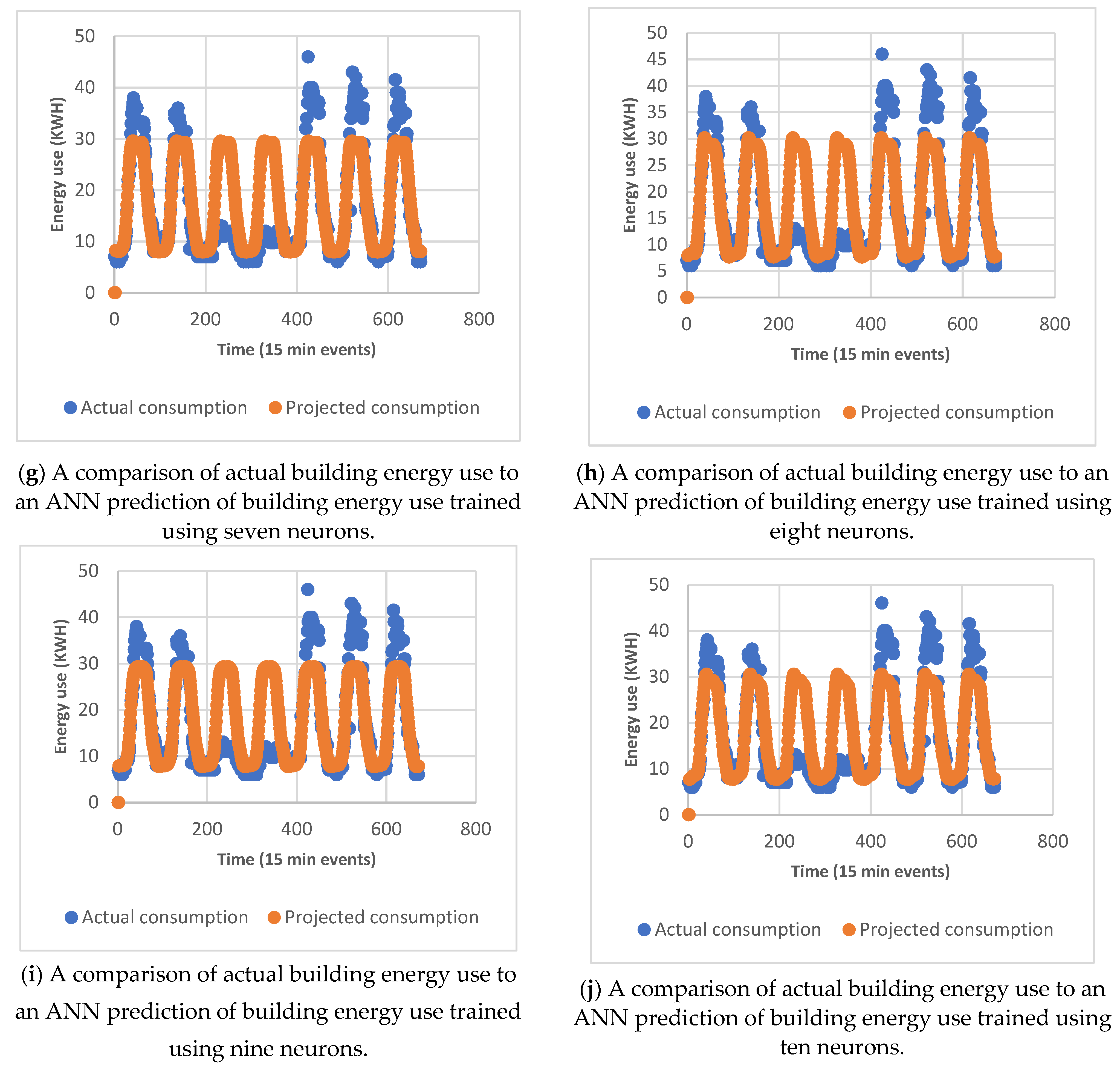
4.1.2. Neuron Selection

Because Levenberg–Marquardt was identified as the optimum ANN, during the selection of the training algorithm, ANNs were trained with the LM training algorithm, using only one hidden layer. One to ten neurons were tested, predicting one day, one week and one month into the future once per season.
Figure 4 shows that by increasing the number of neurons from one to three increased the accuracy of predictions. However, beyond three neurons, accuracy did not increase, and only the time taken to process and predict the data increased. Figure 5 shows the energy predictions using different numbers of neurons.
Because ANNs are considered to be “black box” models, it is unknown why at two neurons, the predictions became flat, i.e., constant. However, it should be noted that the predicted value was the average of all of the energy uses, i.e., 17.81 kWh. A selection of three neurons resulted in the best prediction accuracy, and increasing the number of neurons further only resulted in the same prediction accuracy and a longer convergence time. Additionally, information such as the root mean square error (RMSE) and standard error (SE) of the impact of varying the number of neurons can be found in Table A1.

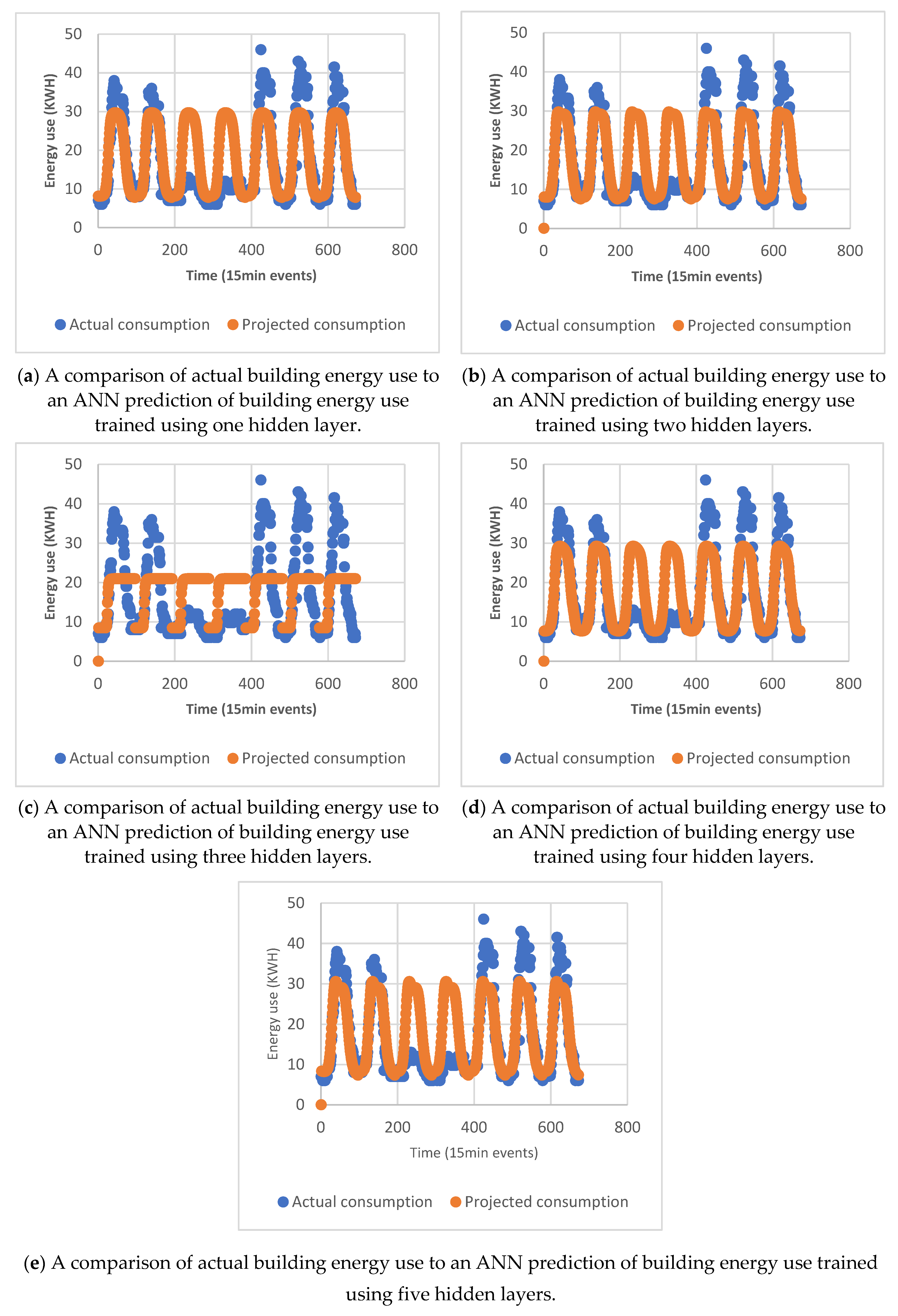
4.1.3. Hidden Layer Selection

Using an ANN with three neurons per layer, and a Levenberg–Marquardt training algorithm, one to five hidden layers were investigated. The results for the monthly predictions are shown in Figure 6.
There was no observed increase or relationship between the number of hidden layers and the predictive accuracy of the ANNs. As such, one hidden layer was selected because it displayed the quickest convergence. This can be explained due to the factors of the limited number of inputs, the size of the datasets, and the respective nature of the data, which did not require additional layers to accommodate their complexity. As a result, the increase in the number of layers did not correlate with the increase in accuracy. However, it was noted that three hidden layers was divergent and produced anomalous predictions with lower accuracy than those with more and fewer hidden layers. Because ANNs are a black box process, it is not known why this occurred when using three hidden layers. Additionally, information such as the RMSE and SE of the impact of varying the number of hidden layers can be found in Table A2.
Other than the anomalous predictions that occurred during the use of three hidden layers, the main variance that occurred between the different number of hidden layers was at the “peak” of their daily predicted energy use. Using five hidden layers, the ANN identified that actual daily energy usage is not a perfect curve that peaks slightly before midday, rather than at midday. This was shown as a small but sharp drop in predicted energy use shortly before midday. This was not observed in the predictions made using four, two or one hidden layers. Despite this, the MAPE from the use of five hidden layers was negligibly different from that from using one layer, despite the increase in computation time. As such, one hidden layer was selected for use in the calibrated ANN.

4.2. SVR Calibration
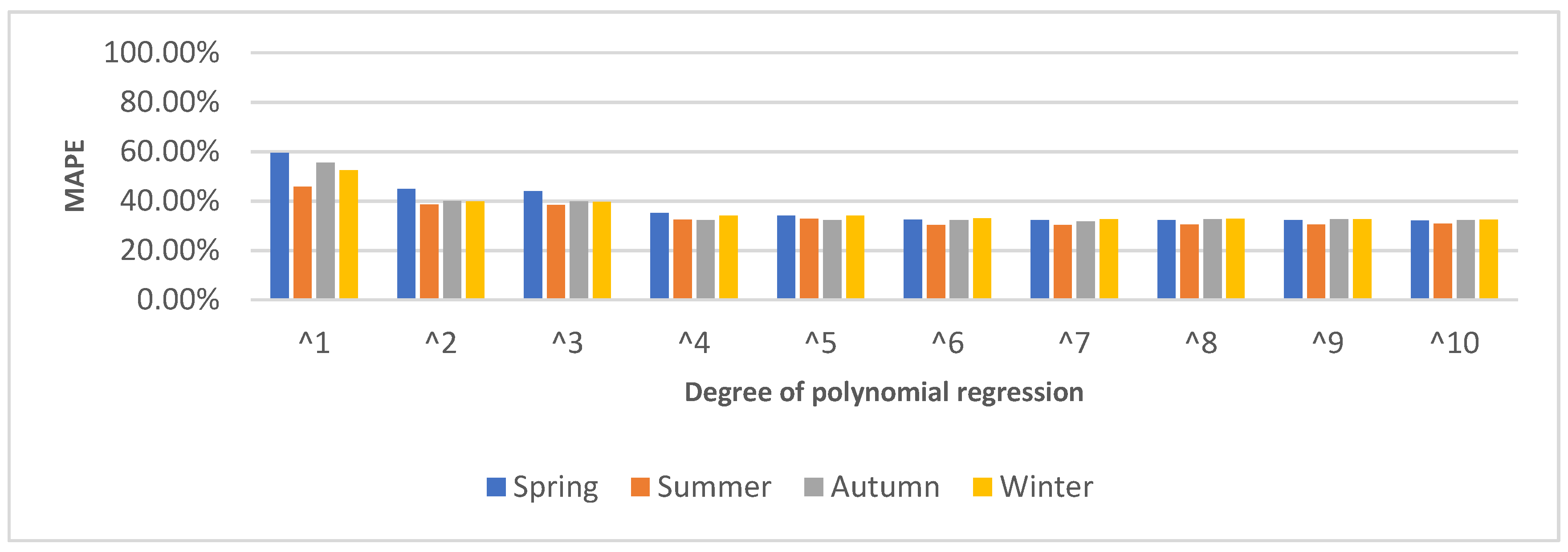
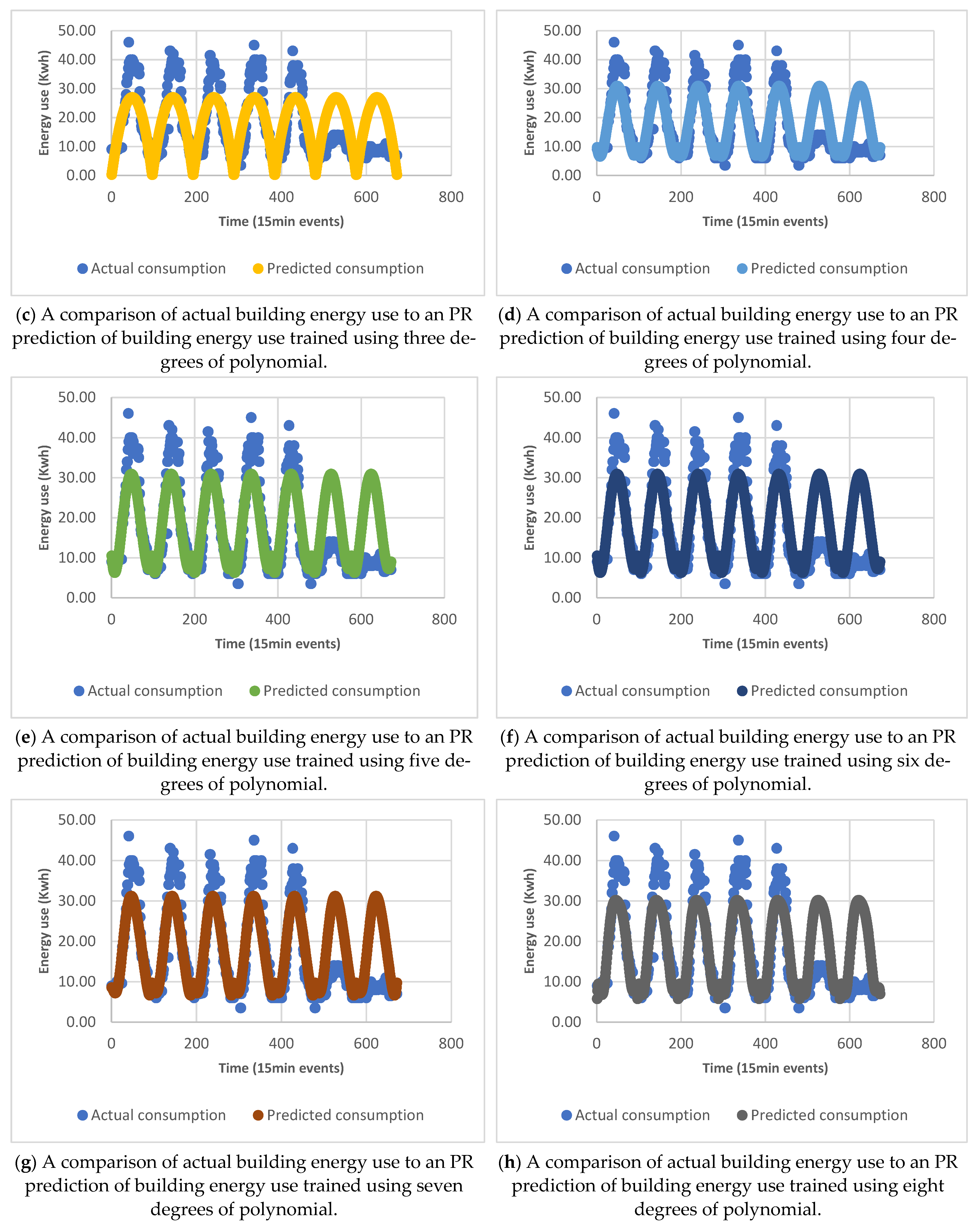
To select a suitable kernel for the SVR model, linear, Gaussian, and polynomial kernels were selected to be tested using the unsegmented data, by comparing their respective MAPEs in predicting monthly building energy use. It was intended that the kernel with the smallest average MAPE would be used in the SVR model for comparative purposes in the later stages of the study. To select a suitable kernel, monthly predictions of each of the seasons were performed with each of the kernels. Linear kernels were discarded early during the model exploration because these resulted in an unacceptably high degree of error, signifying the nonlinear behaviour in the data. Hence, polynomial and Gaussian SVR models were used, and their predictions are presented in Figure 7.
Amongst the two selected kernels, Gaussian SVR models performed significantly (more than 5%) more accurately than the polynomial SVR models, on average. This was because of the poor fit of the distribution of the polynomial predictions to the actual energy consumption. Polynomial kernels had a tendency to return to zero at the end of each day’s cycle, which does not occur in the actual building’s energy usage. Thus, a Gaussian kernel was selected for use in the SVR model in this experiment.

4.3. PR Calibration

To select a suitable regression model for regressing and predicting building energy usage, linear to decic regression models were selected. These were then tested using unsegmented data, by comparing their respective MAPEs in predicting monthly building energy use. The regression model with the smallest average MAPE was used for comparative purposes, as discussed in Section 5. To select a suitable model, monthly predictions of each season were made using a regression of the previous month, by varying the order of polynomial regression from one (linear) to ten (decic), and selecting the order of the polynomial regression with the least MAPE. The range of the order of polynomial regression was increased if the MAPE continued to decrease without plateauing within the initial range.
Figure 8 shows that by increasing the order of regression from one to six, the accuracy of the predictions of monthly energy use increased; however, beyond six degrees, the accuracy reached a plateau. However, the simplicity of regression meant that increasing the order of regression beyond six did not increase the computational time. Because increasing the order beyond six produced only negligible impacts, a sixth-order polynomial regression was selected for use in the experiment’s PR model. Figure 9 shows energy predictions using different orders of polynomials.

5. Results and Discussion

This section explores the impact of seasonality and segmenting training data on machine learning techniques. We investigated and compared the impact of segmenting the training data of PR, SVR and ANNs, into weekday/weekends and building active/dormancy periods, on the MAPEs of building energy forecasts in each season over the range of a month.

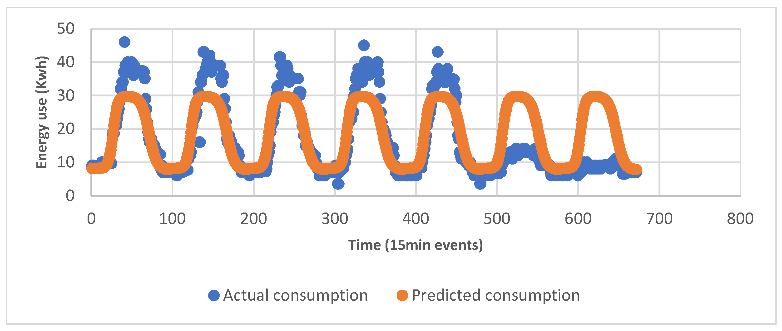
5.1. Forecasting Result Based on Polynomial Regression

This section highlights and discusses the impact of segmenting PR training data into weekday/weekends and building active/dormancy periods in comparison with control non-segmented data.

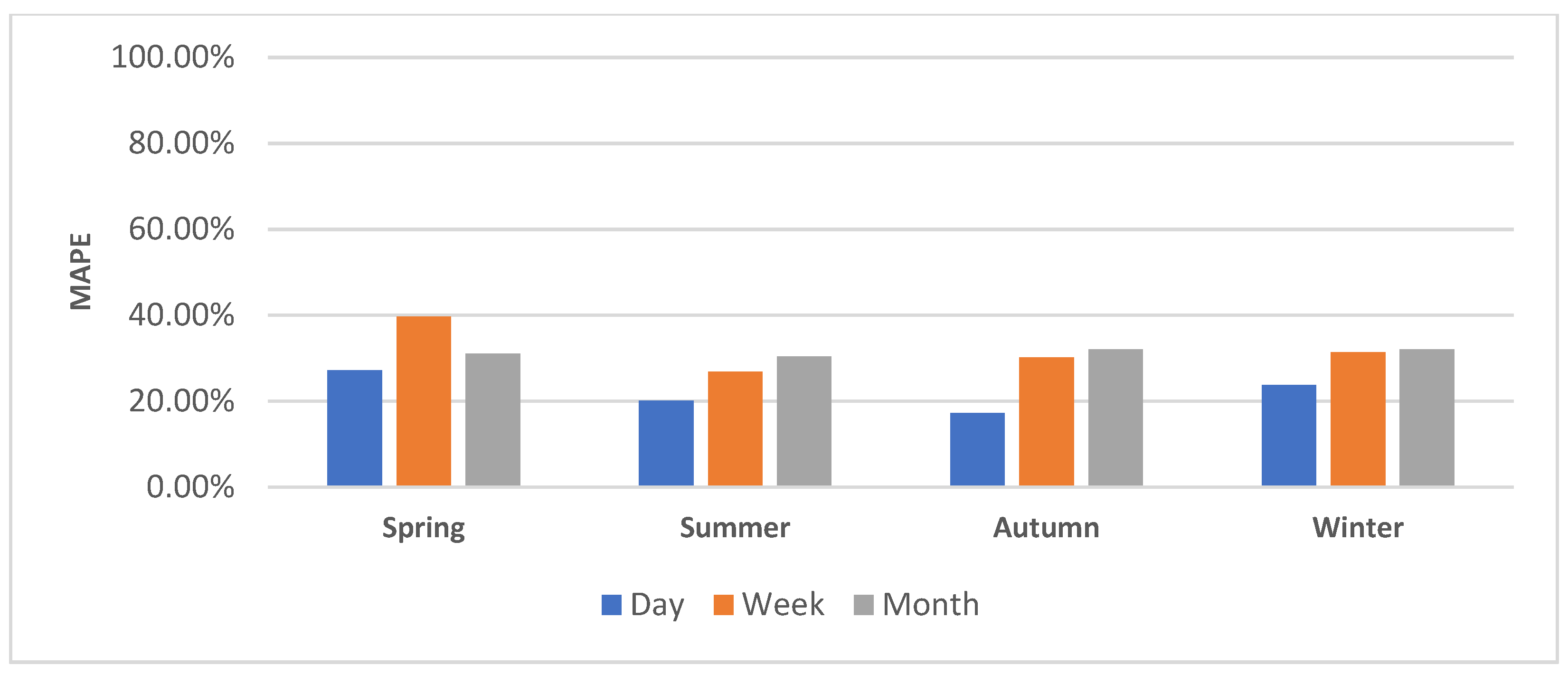
5.1.1. Daily, Weekly, and Monthly Control Building Energy Predictions

Using the previously established PR optimisation, to provide the PR with its “best case scenario”, a PR model using six degrees of polynomial regression was used in the following predictions. Using each season’s monthly training data, the following day, week, and month were predicted. The resulting MAPEs ranged from 17.67% at their lowest in autumn day energy forecasts, to 40.95% at the highest in spring week predictions, with internal ranges of 10.64% in daily predictions, 14.32% in weekly predictions and 2.58% in monthly predictions. These MAPEs are shown in Figure 10.
Figure 10 shows that, with the exception of spring, the MAPE increased as hypothesised, i.e., increasing as the forecast range increased. The increase in MAPE was not proportional to the increase in forecast; for example, the MAPE for a thirty day forecast was not thirty-fold that of a one day forecast. Instead, the bulk of the increase in error occurred in the transition from a one day forecast to a one week forecast, suggesting that greater deviation occurs within each week, than the deviation that may occur between each week. In particular, the spike in inaccuracy occurring in the spring week forecast (and the spring day forecast), contributed to the largest range in accuracy of 14.37% between the spring and summer forecast (and the large range in the daily forecast MAPE of 10.64% between spring and autumn predictions). The increase in the deviation in spring did not continue into the monthly forecast, where the greatest range between MAPEs was significantly smaller at 2.57%, and occurred between winter and summer forecasts. The fact that spring no longer contributed to the maximum range of the MAPEs at the monthly level, with such a low range in place, highlights that the main cause of the deviation from the training data in spring occurred within the first week of the spring test period. This was confirmed upon conducting data exploration of the testing data. As shown in Figure A5, the first week of spring did not feature a consistent incline towards “peak” midday energy use. In contrast, the energy use spiked to reach its peak immediately after the building left its dormancy state, which may have been due to a heat spike leading to an increase in HVAC usage.

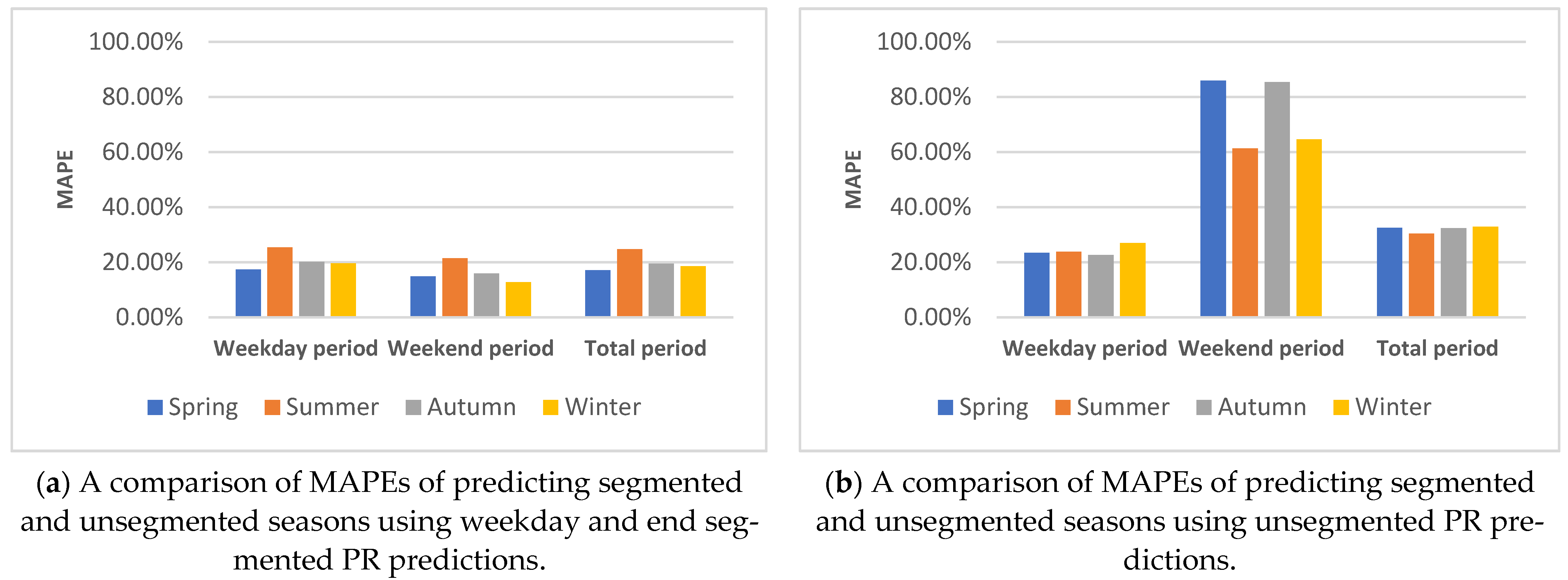
5.1.2. Weekend and Day Data Segmentation

From each of the training months of each season, four segmented training sets and one control sets were constructed. These segmented training sets were then used to train models to predict the same segment of the month in the following month of the season. The MAPEs of these predictions were then compared with the MAPEs of the predictions of the model trained using unsegmented data, to predict the same segments predicted by the models trained with segmented data. Figure 11 compares the resulting MAPEs of the models trained using weekday and weekend data with those of the predictions of the weekday and weekend produced by the control model. The total period refers to the MAPE that occurred over the entirety of the forecast range, regardless of the segments that may occur within them.
As presented in Figure 11, segmenting the training data between weekdays and weekends, and modelling them separately, produced a significant reduction in MAPE across all predictions (with the exception of summer weekday predictions). The most significant reduction in inaccuracy occurred in weekend predictions. As can be observed in Figure A6, the segmentation of the training data allowed for a greater level of specialisation in the PR models. This enabled the segmented PR models to independently map the different energy usage patterns of the weekday and weekend periods, rather than averaging the two to produce a model capable of predicting both. In turn, this allowed for a better reflection of the low energy use occurring during weekends due to lower building occupancy and activity. Conversely, as a result of the removal of the weekends from the weekday models, the weekday models increased the size of their predicted peaks, in accordance with actual weekday energy use, thus increasing overall accuracy.
The small peaks in both unsegmented and segmented results (in grey and orange), shown around times 100, 195, 290, 385 and 580 in Figure A6, occur in the region of the cross-over between the days of the week at midnight. Following data exploration, it was identified that these peaks were due to the manner in which the specific time of day (00:00 to 24:00) was interpreted numerically in the datasets (0 to 1). Due to the manner in which time was interpreted linearly, rather than cyclically, and due to the slight variance in the timing of the trough in building energy use during training, the model did not recognise that a smooth trend should exist between the predicted events before and after midnight. Rather, the incline towards the following day started early, and the decline from the previous day occurred later, both to a minor degree, compared to the actual inclines and declines.

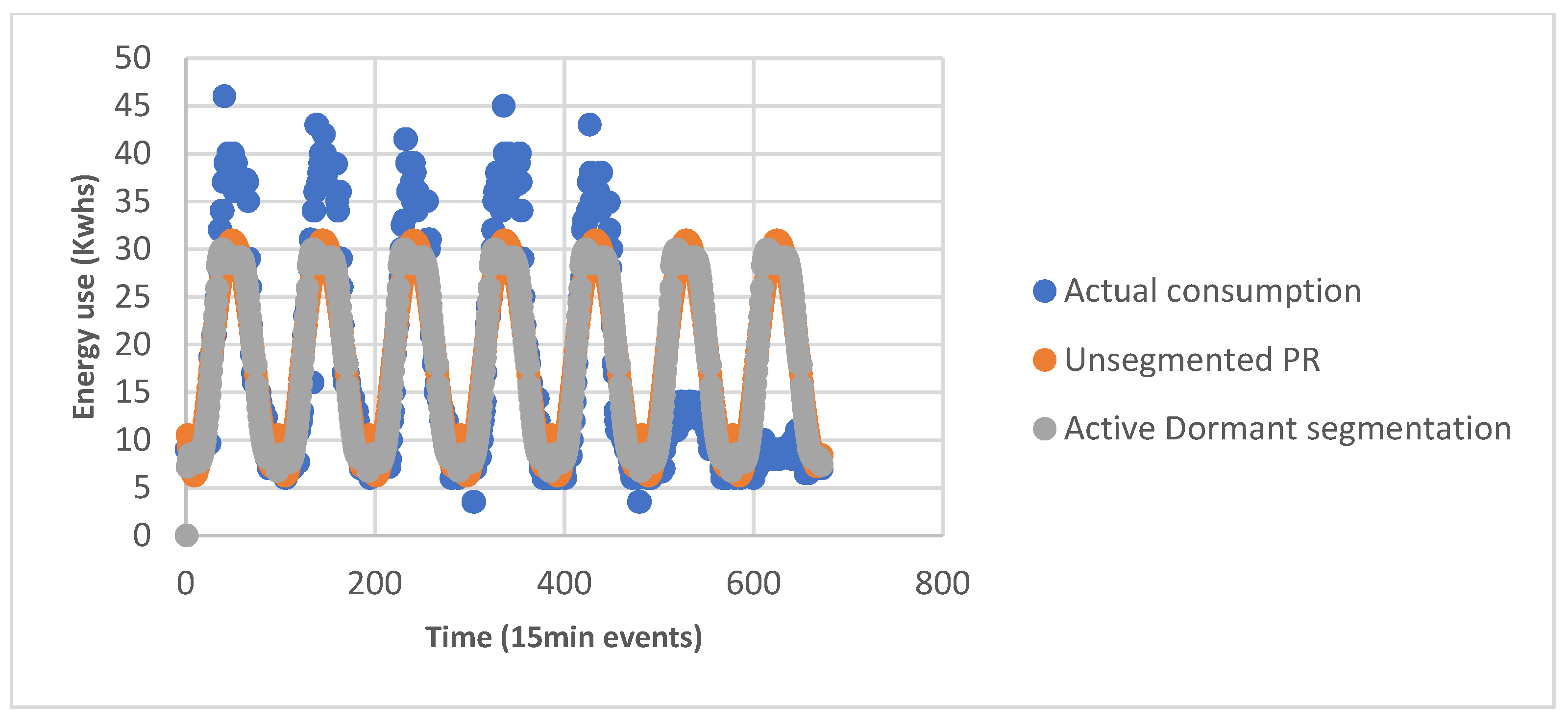
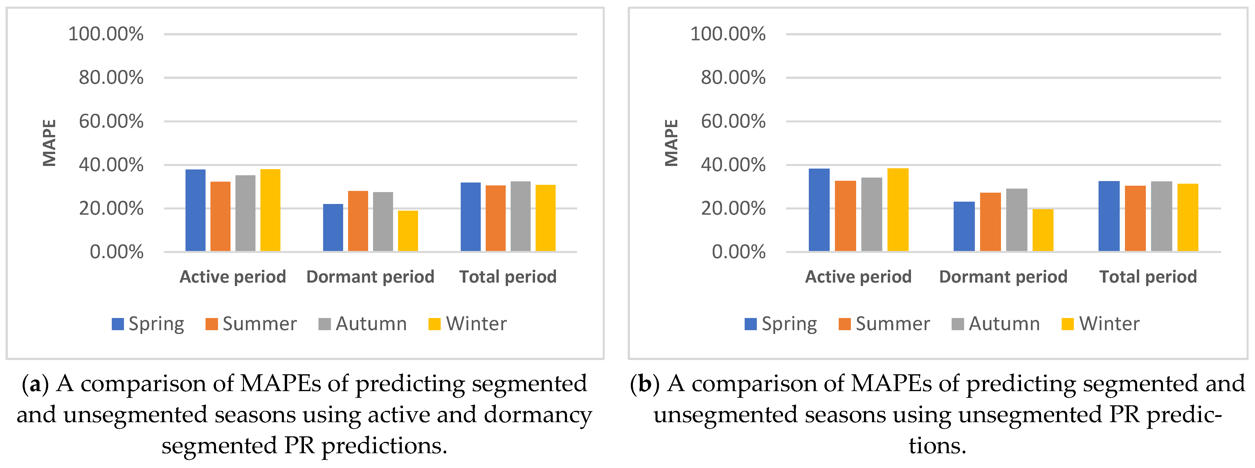
5.1.3. Active and Dormancy Period Segmentation

As stated in Section 5.1.2, from each of the training months of each season, four segmented training sets and one control set were made. These segmented training sets were then used to train models to predict the same segment of the month in the following month in the season. The MAPEs of these predictions were then compared with the MAPEs of the predictions of the model trained using unsegmented data, to predict the same segments predicted by the models trained with segmented data. In Figure 12, the resulting MAPEs of the models trained using building active and dormancy periods are compared with the predictions of the building active and dormancy periods produced by the control model. The total period refers to the MAPE of the entirety of the forecast range, regardless of the segments that may occur within them.
As can be observed in Figure 12, although weekend weekday segmenting reliably increased the accuracy of PR’s building energy predictions, segmenting by building active and dormancy periods had an erratic effect on prediction accuracy, averaging to a net negative. This was in contrast to the previous observations when predicting specific meters, where the prediction accuracy of the Clarendon building’s cooling system was increased by building active/dormancy period segmentation, thus highlighting the difference between the pattern of building HVAC energy use and net energy usage. Figure A7 demonstrates that segmenting by building active period and building dormancy period did not lead to any significant changes in the pattern of PR-predicted building energy use. Additionally, it demonstrates that, in net building energy usage, dormancy and active energy use are part of the same pattern of energy use. Rather than a set rise or drop in energy use occurring between the two periods, the two periods phase in and out of each other.

5.2. Forecasting Result Based on Articifial Neural Networks

This section highlights and discusses the impact of segmenting ANN training data into weekday/weekends and building active/dormancy periods in comparison with control unsegmented data.

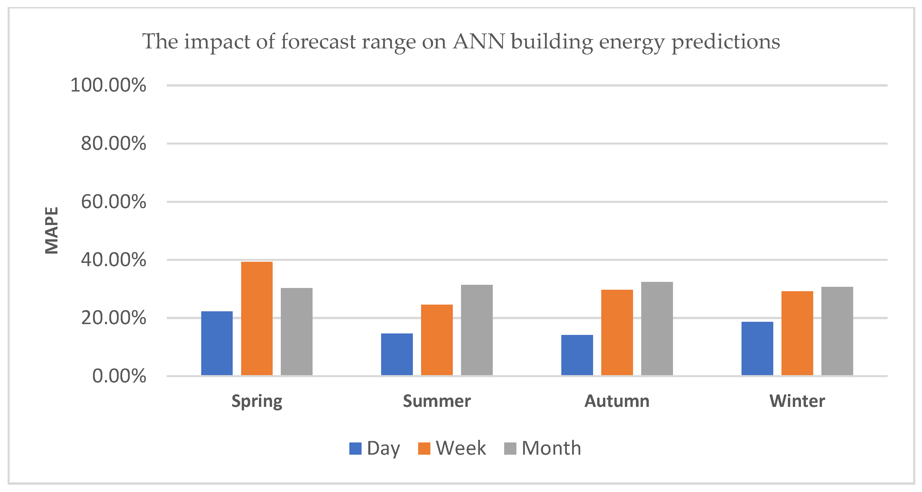
5.2.1. Daily, Weekly and Monthly Control Building Energy Predictions

Using the previously established ANN optimisation to provide the ANN with its “best case Scenario”, an ANN with three neurons, one hidden layer and trained with the Levenberg–Marquardt algorithm was used in the following predictions. Using each season’s monthly training data, the following day, week and month were predicted. The resulting MAPEs ranged from 17.26% at their lowest in autumn day energy forecasts, to 39.65% at their highest in spring week predictions, with internal ranges of 9.88% in daily predictions, 12.83% in weekly predictions and 0.95% in monthly predictions. The resulting MAPEs are compared in Figure 13.
As previously seen in the PR predictions of building energy usage, it can be observed that, with the exception of spring, the MAPE increased as hypothesised, increasing as the forecast range increased. The MAPE increased predominantly with the expansion of the forecast range from day to week, rather than from week to day. The same spike in error occurred during the spring week and day forecasts, indicating that the specific spike in MAPE is the result of the data, rather than any specific machine learning technique’s ability to predict the data. However, when using ANNs, the range and overall scale of the errors was mildly reduced compared to when using PR. For example, the range of errors was reduced to 9.88% between spring and summer in day forecasts, 12.38% between spring and summer in week forecasts, and to a minimal range of 1.68% between autumn and summer monthly forecasts. This highlights a pattern in which summer is the best season to predict data. ANN predictions at this stage are unable to accommodate for the peaks of weekday energy use, or the low day time energy use occurring on weekends, as shown in Figure A8.

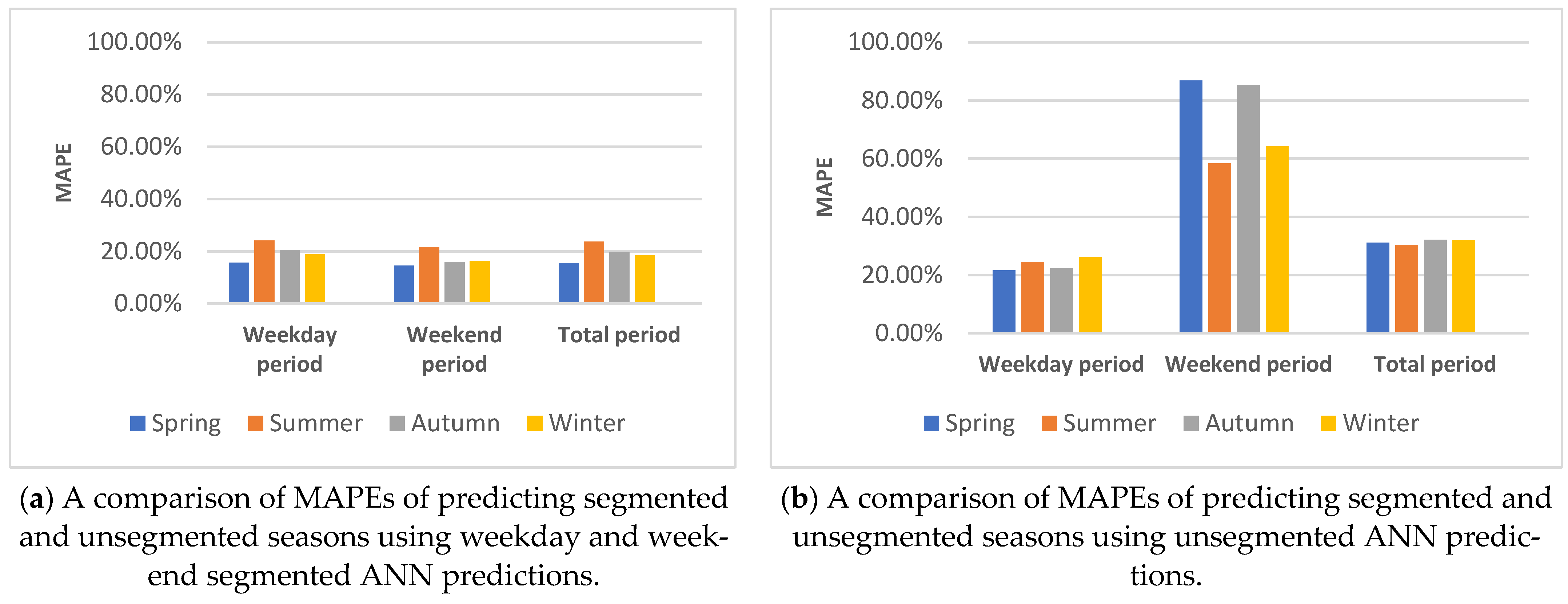
5.2.2. Weekend and Day Data Segmentation

In Figure 14, the resulting MAPEs of ANN models trained using weekday and weekend day are compared with the predictions of the weekday and weekend produced by the ANN control model.
As presented in Figure 14, segmenting the training data between weekdays and weekends, and modelling them separately, produced a significant reduction in MAPE across all predictions, with the same exception of summer weekday predictions as observed in Figure 11. Segmenting the data into weekends and weekdays resulted in lowering the MAPEs of the ANN models to similar levels as observed in daily forecasting. The most significant reduction in inaccuracy occurred in the weekend predictions, as observed in Figure A9, where the weekend segmented model more closely aligns with weekend energy use than the control ANN model, although the weekend/weekday ANN is not able to accurately predict the highest peaks of weekday energy use. The largest reductions in MAPE of 72.40% and 69.39%, respectively, can be observed in the weekends of spring and autumn, with summer having the least reduction in weekend MAPE of 36.69%. The finding that summer had the smallest reduction in MAPE during weekends from weekend segment models is predominantly due to the higher building energy usage that occurs on Saturdays during summer. As a result of this higher energy use on Saturdays, which is likely due to increased building use during summer activities, the energy use of the weekend period is similar to that of weekdays, thus reducing the difference between the weekend and weekday building energy use patterns. The increased similarity in building energy patterns results in less error in the unsegmented predictions, thus reducing the scope of the segmented models to improve predictive accuracy.

5.2.3. Active and Dormancy Period Segmentation

Figure 15 compares the resulting MAPEs of the ANN models trained using building active and dormancy periods with the predictions of the building active and dormancy periods produced by the control model.
Segmenting into active and dormant periods resulted in no significant change in accuracy (less than 5%) across all predictions, with a decrease in the MAPE of 0.35%, on average, among the total MAPE of the forecasted periods. This decrease in MAPE is potentially due to the randomly selected nature of the data used to train, validate and test the training model, given the small size of the variances. It can be noted that the active dormancy ANN model is poorly aligned with the actual energy consumption where the actively trained model meets the inactively trained model at 18:00–18:15. This lack of connection in the predicted building energy usage, which creates a gap that does not follow actual building energy usage, can be observed in Figure A10.

5.3. Forecasting Result Based on Support Vector Regression

This section highlights and discusses the impact of segmenting weekday/weekends and building active/dormancy periods in comparison with the control unsegmented data on SVR building energy forecasts.

5.3.1. Daily, Weekly and Monthly Control Building Energy Predictions

Using the previously established SVR optimisation, to provide the SVR with its “best case scenario”, a SVR model using a Gaussian kernel was used in the following predictions. Using each season’s monthly training data, the following day, week and month were predicted. The resulting MAPEs ranged from 18.58% at their lowest in summer day energy forecasts, to 39.27% at their highest in spring week predictions, with internal ranges of 3.71% in daily predictions, 14.69% in weekly predictions and 2.13% in monthly predictions. These MAPEs are presented in Figure 16.
As shown in Figure 16, with the exception of the daily and weekly spring forecasts, the SVR forecasting error increased with the forecasting range. Most of the increase in the error occurred between the shift from daily forecasts to weekly forecasts. This again confirms that the minor drift in building energy use due to seasonality that occurs between weeks over a monthly period causes less variation in the data, than the variations in building energy use that occur between the days of the week. These variations in daily building energy use over the course of a week are shown in Figure A11. As can be observed on a weekly basis in Figure A1, Figure A2, Figure A3 and Figure A4, the two lower peaks between event 500 and 700 in the daily actual building energy use in Figure A11 are the result of reduced building activity during the weekend periods. The forecast is unable to accurately predict the weekend period because the forecasting model needs to accommodate both the weekend and weekday periods. Because the weekday period is larger than the weekend period, the average prediction is weighted in favour of the weekdays.

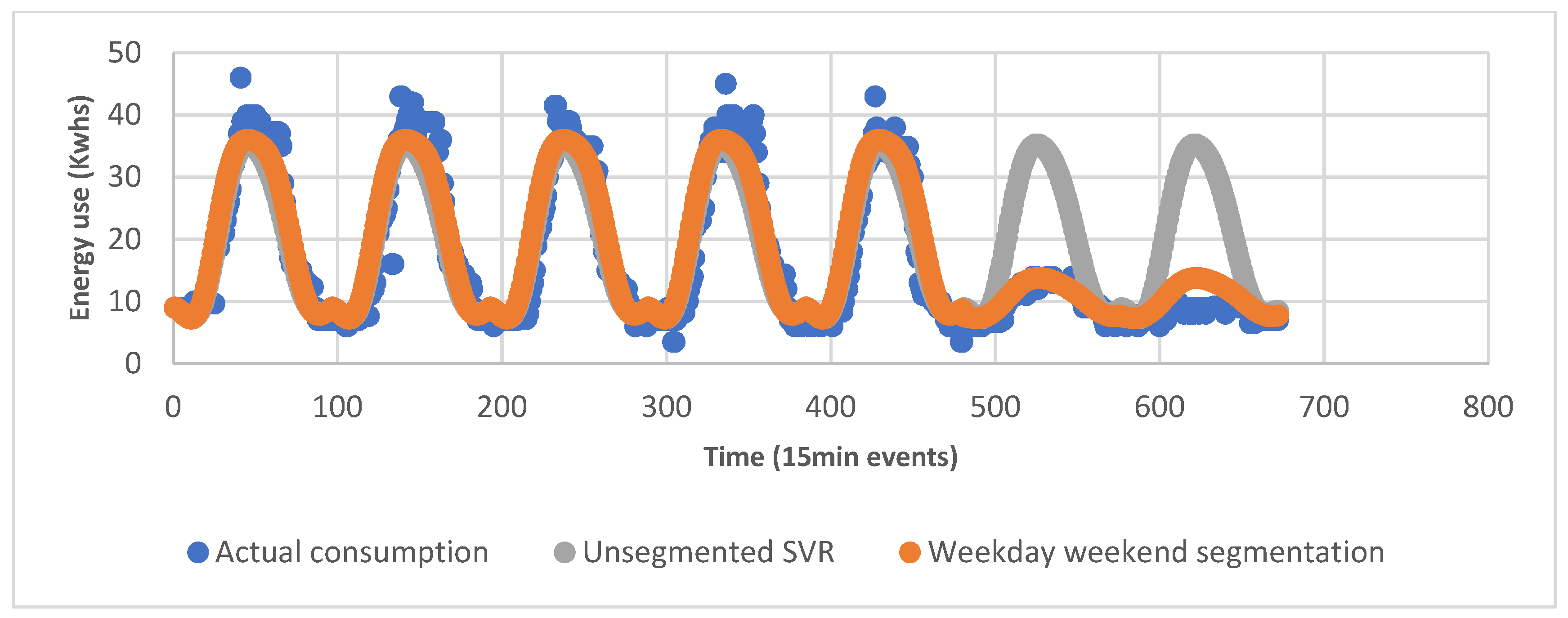
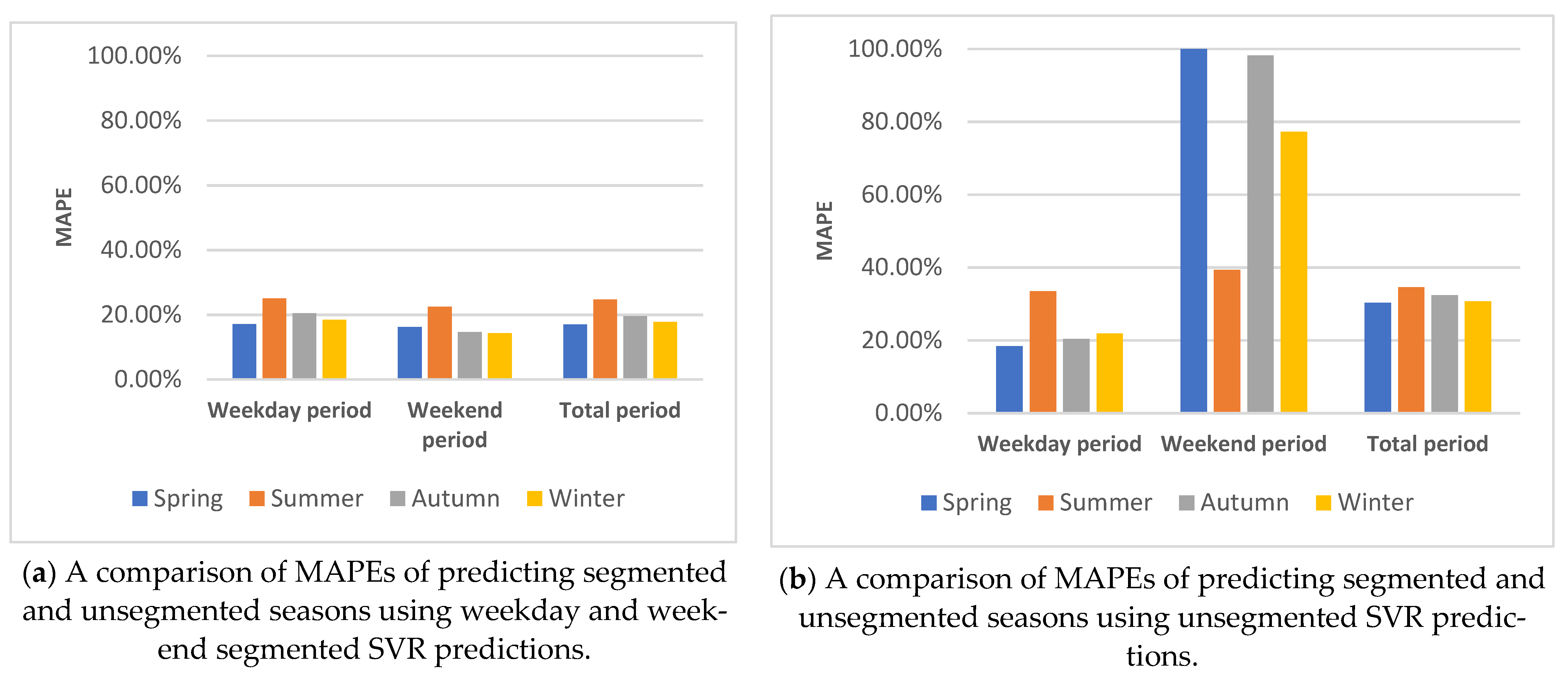
5.3.2. Weekend and Day Data Segmentation

In Figure 17, the resulting MAPEs of the SVR models trained using weekday and weekend data are compared with the weekday and weekend predictions produced by the control model.
As is shown in Figure 17 (and Figure A12), using a weekday and weekend model to forecast building energy use resulted in greater accuracy for predictions of the distinct building energy use periods. This was due to removal of the main source of deviation in the weekly cycle, which would be required to be accommodated by a singular forecast. Weekday/weekend segmentation resulted in a decrease in the average MAPE of monthly predictions from 31.18% to 19.73%, making it more accurate than unsegmented weekly forecasts (30.65%). However, the unsegmented daily prediction was 2.33% more accurate than the monthly weekday/weekend segmentation forecast. This is hypothesised to be due to either the drift in HVAC energy usage from the training period caused by changes in weather patterns, or changes in build use occupancy patterns caused by holidays and lesson scheduling (because the main source of error from weekend/weekday differences was removed).

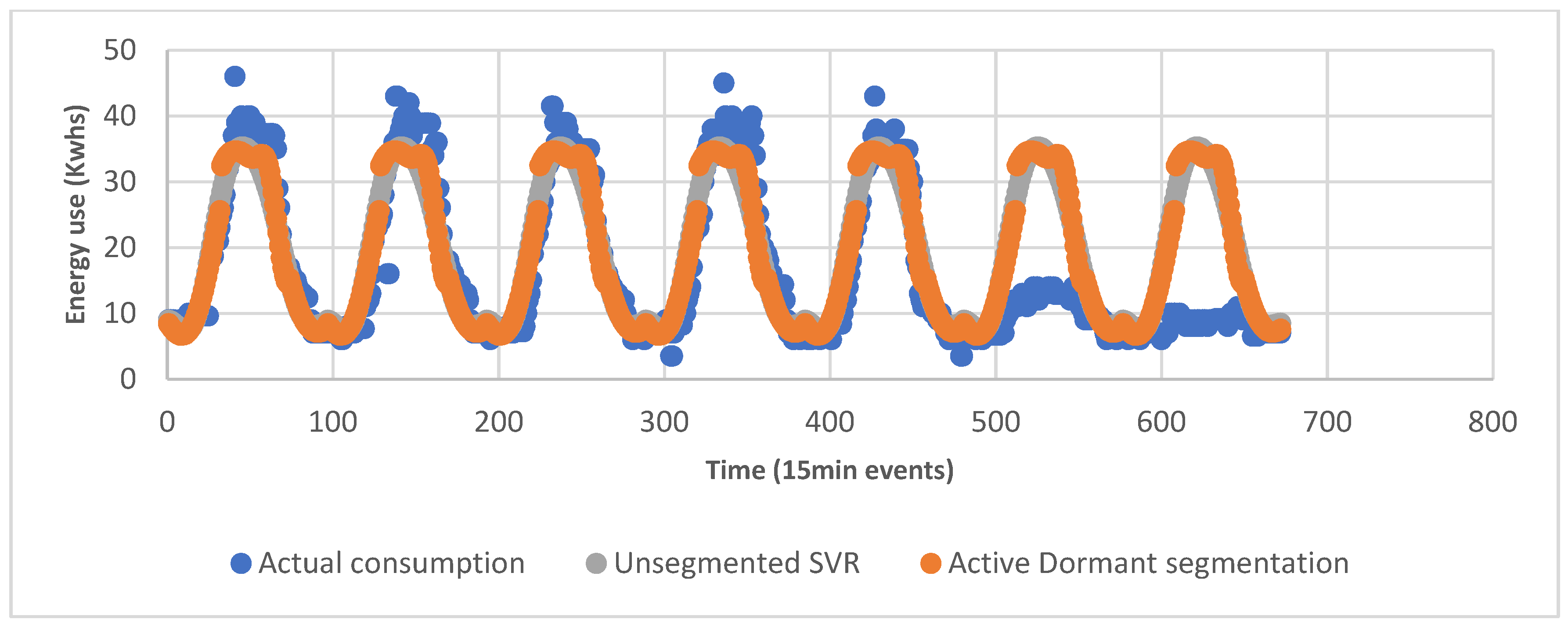
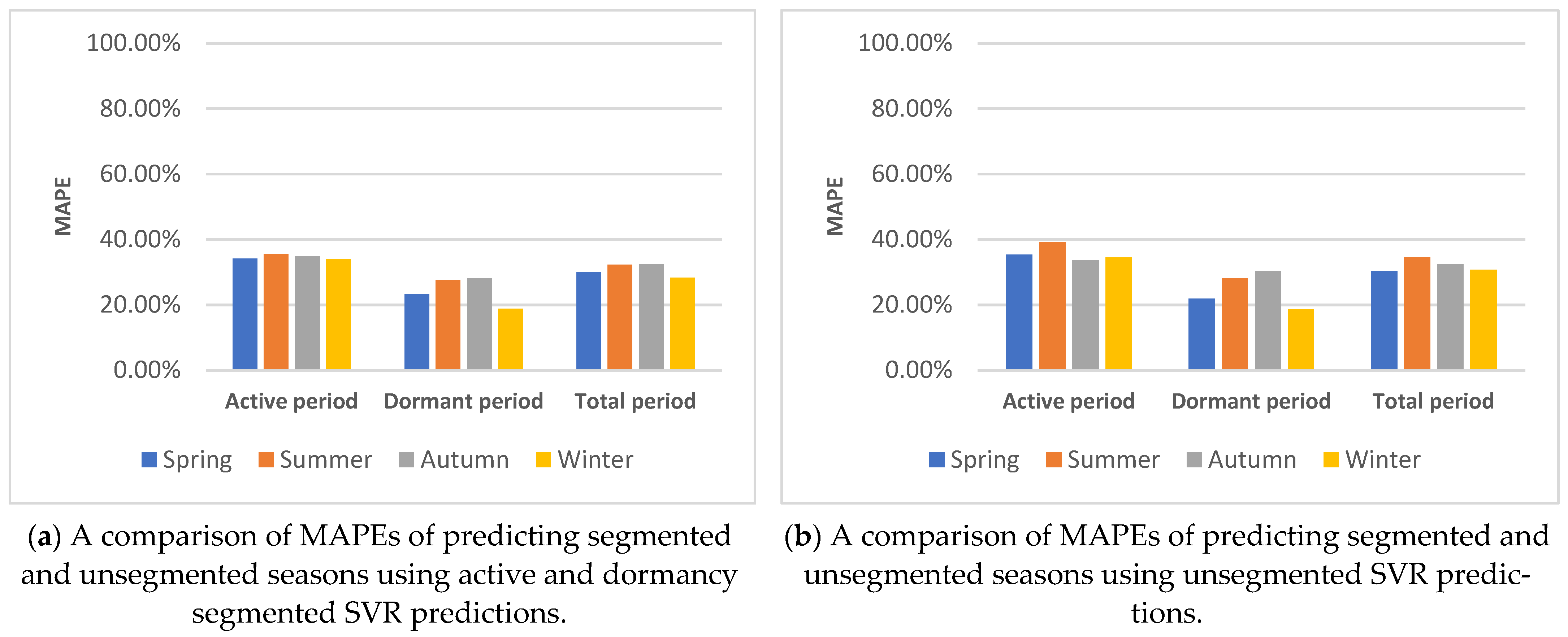
5.3.3. Active and Dormancy Period Segmentation

Figure 18 compares the resulting MAPEs of the SVR models trained using building active and dormancy periods with the predictions of the building active and dormancy periods produced by the control model.
As can be observed in Figure 18 (and Figure A13), building active and dormancy period segmentation had a negligible impact (<5%) on the accuracy of the SVR building energy predictions. In previous studies that produced predictions for the Clarendon building’s chiller system, it was found that segmentation into building active and dormancy periods improved forecast accuracy. This discrepancy between the two studies is most likely due to the difference in energy usage between the building’s chillers and the building’s total energy use; whereas the chillers have a distinct on/off transition, and a clear divide between the active and dormancy periods, the building’s total energy use is a continuous pattern of peaks and troughs. Unlike the previous (PR and ANN) building active/dormancy segmented models, the “gap” during which the active and dormancy periods meet occurs within the range from 07:45 to 08:00. This contrasts with previous similarly segmented models, in which this gap occurred in the range of 18:00–18:15.

5.4. Comparison and Discussion

Here, we present the collected results from the “best case scenario” of each of the tested machine learning techniques, for use in comparison and determination of the most accurate technique under a range of circumstances.

5.4.1. Daily, Weekly and Monthly Predictions

Using the “best case scenario” predictions from Section 5.1.1, Section 5.2.1 and Section 5.3.1, the daily, weekly and monthly forecast MAPE values of each machine learning technique are presented for their respective seasons in Figure 19.
For short-term daily predictions, it can be observed in Figure 19 that SVR reliably performs most accurately in each season, with the smallest variance in the accuracy of the three techniques observed, followed by the ANN and then PR. This is consistent with historical examples, in which SVR has traditionally outperformed other machine learning techniques in the prediction of short-term building energy loads. Similarly, regarding the daily predictions, at the weekly forecast range it can be observed in Figure 19 SVR reliably performs most accurately in each season; however, as the forecast range increases, the difference between the MAPEs of SVR and ANN predictions decreases, such that the difference in accuracy is represented by an MAPE difference of only 1.35% on average. The trends of SVR performing most accurately, on average, and the difference between the MAPE of SVR and ANN predictions decreasing as the forecast range increases, was also found in the monthly predictions, as shown in Figure 19. However, at the monthly forecast range, the difference in the accuracy between ANN and SVR is insignificant (<5%), represented by a difference in the MAPE of 0.7%, and there are two examples in which the ANN predictions are more accurate than SVR predictions. In contrast, in summer and autumn, the ANN model was 1.06% and 0.37%, respectively, more accurate than the SVR model. There is a possibility that the ANN model would be more accurate than SVR at increased forecast ranges if the trend continued. However, at these increased ranges, the MAPE would likely be beyond an acceptable threshold for use in prediction purposes, thus limiting its practical use.

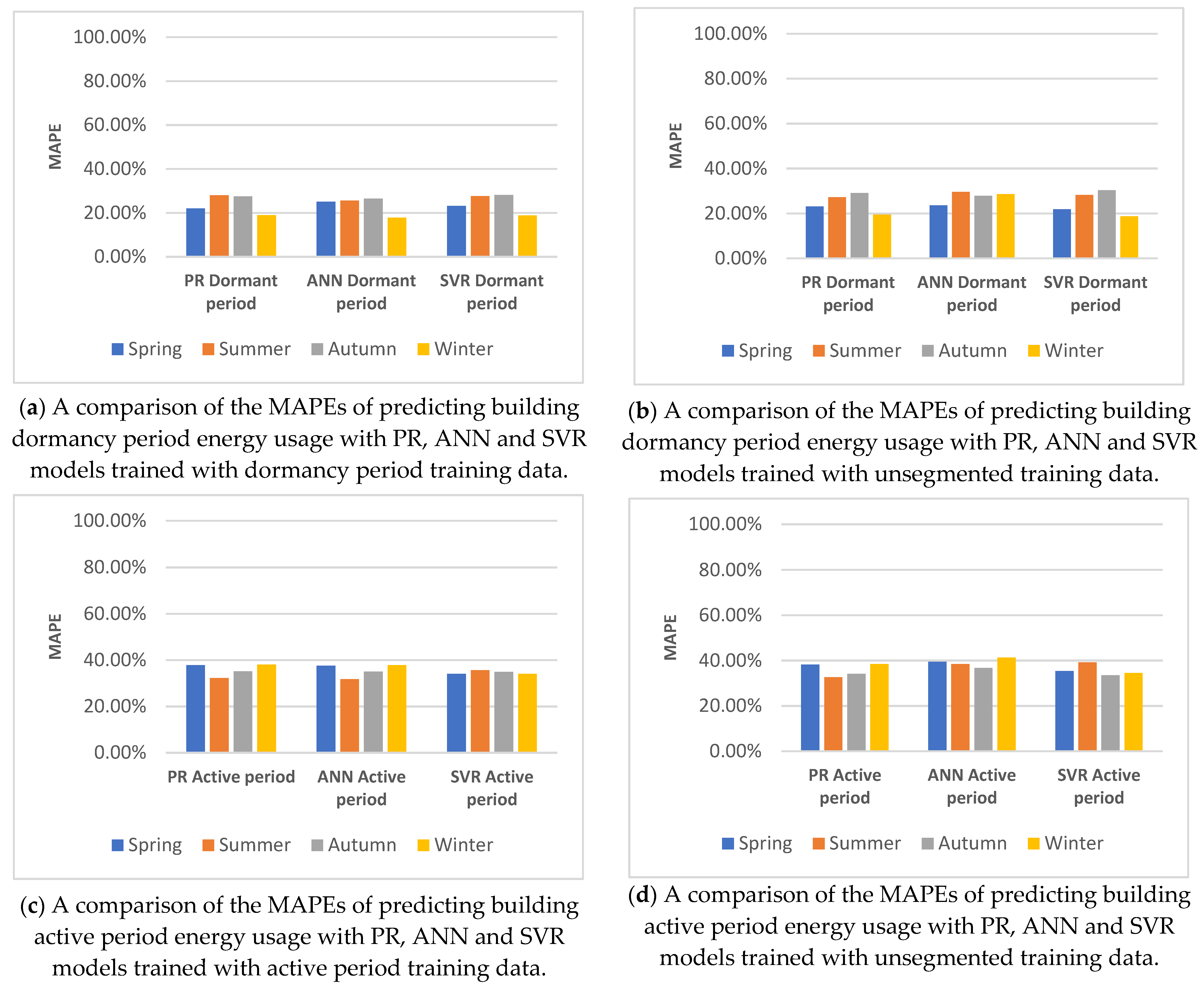
5.4.2. Building Active/Dormancy Segmented Predictions

Segmenting the energy prediction models by building active and dormancy periods decreased the MAPE of PR, SVR and ANN models by, on average, 0.24%, 0.12% and 0.32% respectively, as shown in Figure 20. However, the magnitude of these reductions was negligible and sufficiently small that they may be attributed to the randomness of the data selected to train the model, and the data used to validate it. Similarly, relative to the monthly predictions produced by the control, the accuracy of SVR was greatest, followed by that of the ANN, by a very small margin (0.49%), on average.

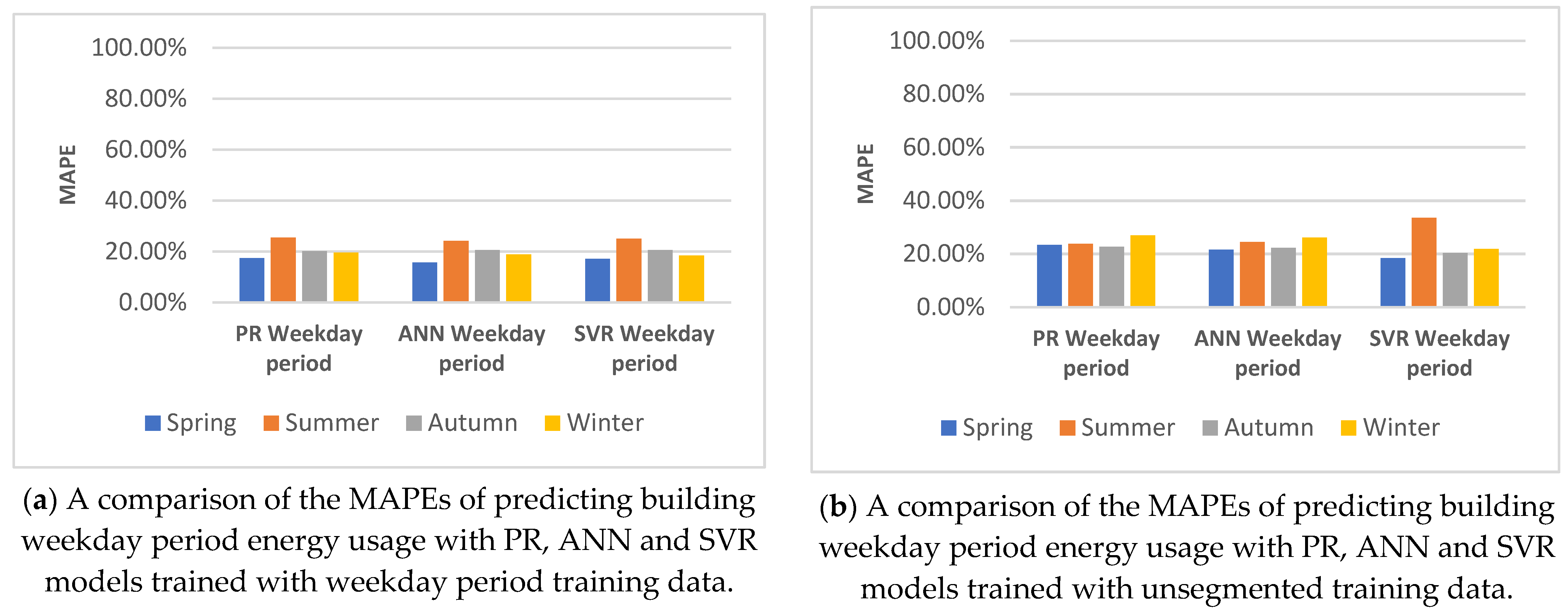
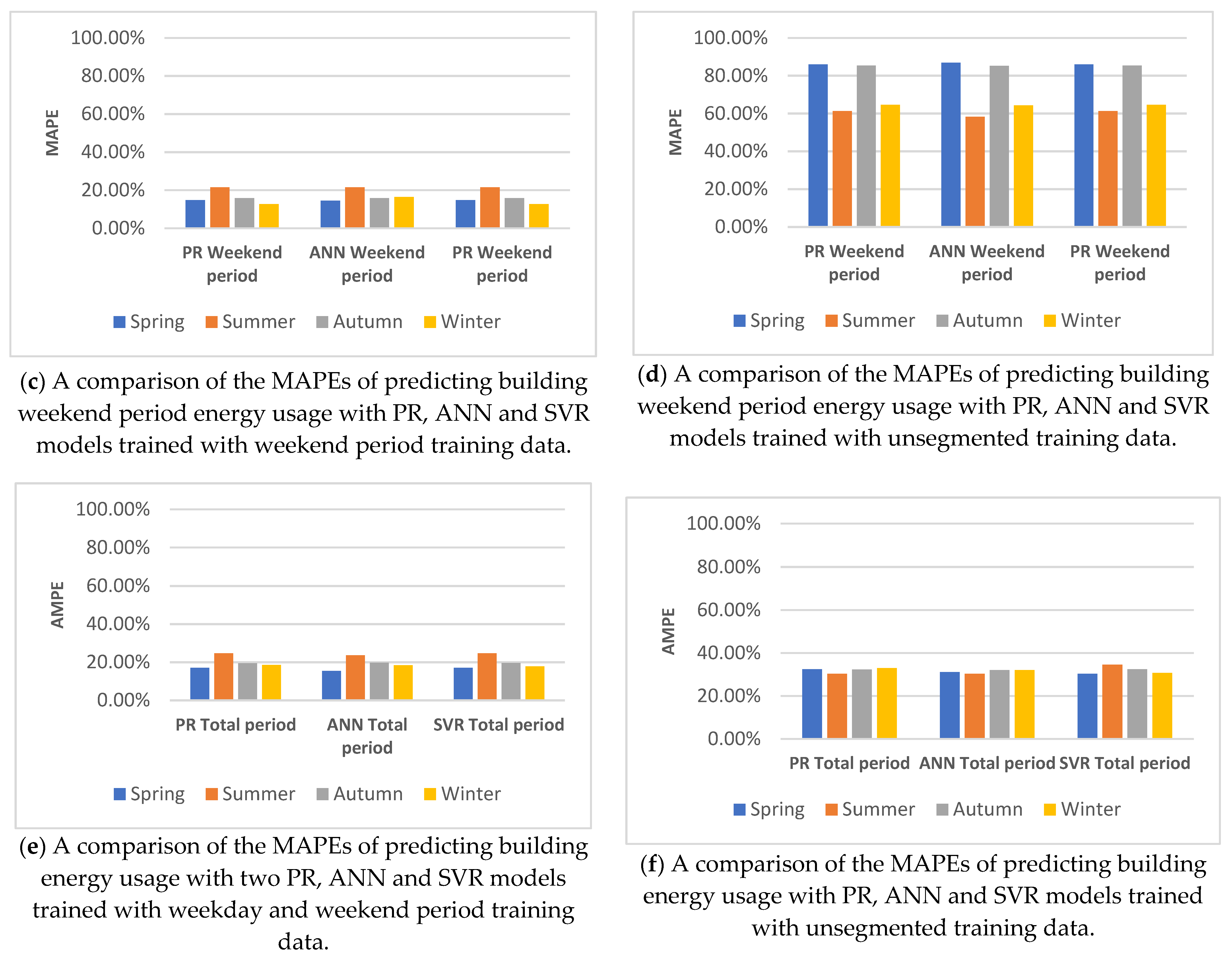
5.4.3. Building Weekday/Weekend Segmented Predictions

Conversely to the building active/dormancy period segmentation, segmenting by weekdays and weekends significantly (>5%) reduced the MAPE of all of the tested machine learning techniques, as shown in Figure 21. The overall MAPE of PR, SVR and ANN predictions was reduced by over 10% in all cases, such that the ANN prediction was more accurate than the SVR prediction by 0.41%. This was the first case in which any other technique outperformed SVR, on average. This highlights that, although data segmentation can be used to improve a model’s accuracy, it is highly dependent on the basis on which the data is segmented. In cases in which there is a significant difference between the behaviour of the Clarendon building’s energy use, such as in the case of weekdays and weekends, segmentation improves the model’s accuracy. However, where the data follows a continuous pattern, such as between building active and dormancy periods, segmentation decreases the model accuracy.
As can be seen in Figure 22, which compares the weekday and weekend building energy usage during the first week of autumn, the two different behavioural patterns of building energy use can be clearly observed. Energy use during weekday periods reached 46 kWh, whereas weekend energy use did not exceed 13 kWh. Similarly, Figure 22 also highlights the issues associated with segmenting the active period from 8:00 am to 18:00 pm (and the active period of the building’s cooling systems [44]). Although this period represents the bulk of occupancy, and contains the spikes in energy use due to students, it does not effectively divide the data into separate energy use patterns or produce datasets that are significantly easier for a machine learning technique to map.

5.4.4. Impact of Seasonality on Prediction Results

Although seasonality had a different impact on all of the predictions of each machine learning technique, forecasting range and data segmentation, certain trends emerges. In all unsegmented medium- and long-term forecasts, summer predictions had greater accuracy than spring, autumn and winter forecasts. Summer predictions were only outperformed by autumn predictions in the PR, ANN and SVR daily predictions (by 1.45%, 2.86% and 0.46%, respectively). On average, the performance of the two autumn periods was 1.57% worse than that of the summer predictions. Compared to the summer predictions, the performance of the winter predictions was 4.73% worse and that of the spring predictions was 8.54% worse.
The initial assumption was that this was due to changes in the building energy usage that occurred month-to-month due to changing weather patterns and external temperatures. For example, as the temperature increases in spring, less energy is spent on heating by the building’s HVAC system. This would be difficult to predict by the models if the heat load dropped below that recorded in any historical training data. However, the comparison of the differences in the average energy use between each season’s monthly training and testing data shown in Table 1 shows that, rather than summer having the smallest differences between the mean energy use, and spring having the largest, spring had the smallest differences, and summer was ranked second. In Table 1, a negative value is the result of the testing value being smaller than the training value, and a positive value is the result of the testing value being larger than the training value.
This suggested that the 8.54% difference in prediction accuracy between summer and spring occurred for reasons other than a net shift in building energy usage. Data exploration of the actual building energy use revealed three points of interest between the spring and summer data testing sets:
-
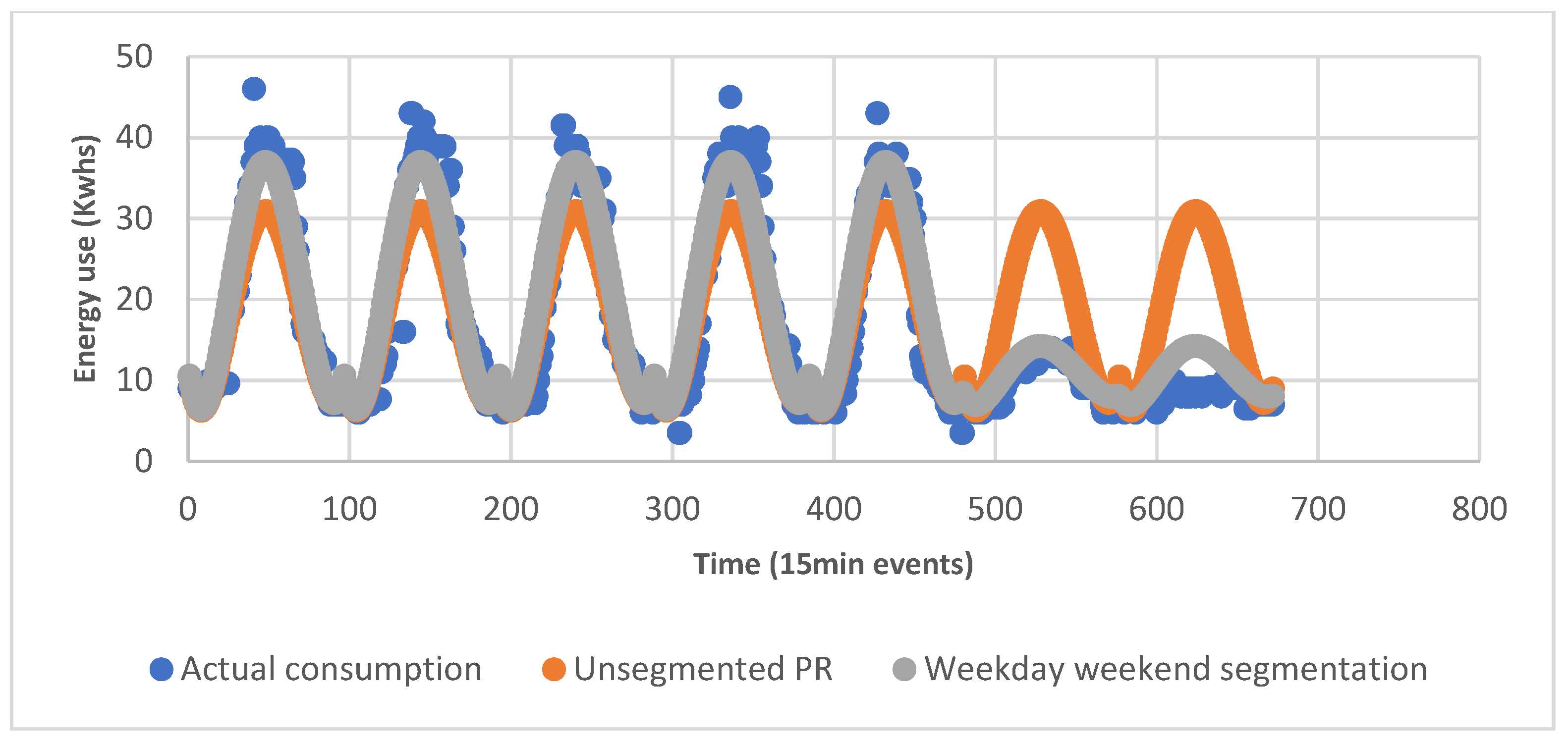
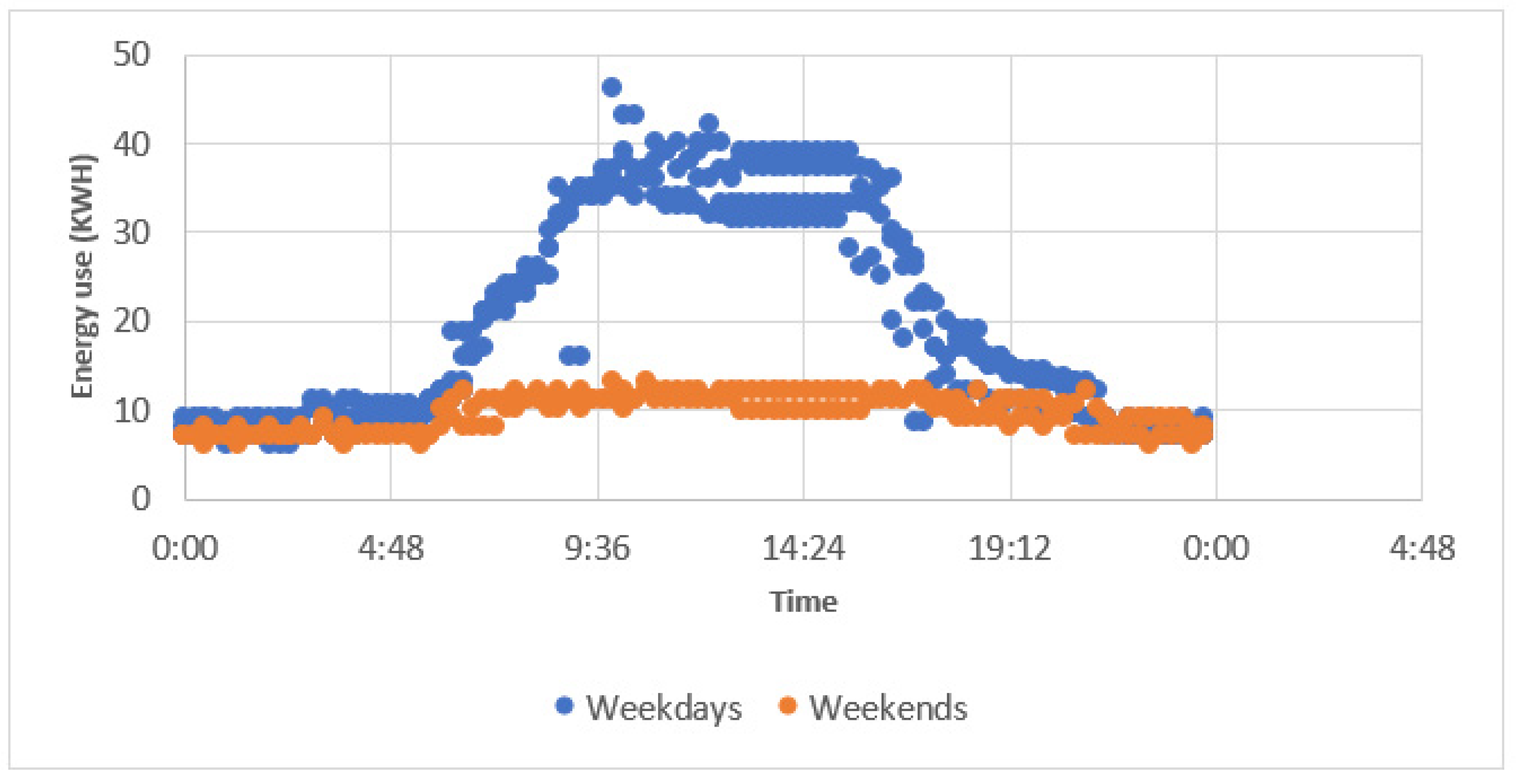
During weekdays, the Clarendon building had higher peaks of energy use during the spring than the summer. There was a three day dormancy period in the first two weeks of the spring period that disrupted the normal building energy usage patterns. Removing this period from long-term spring ANN predictions (the most accurate predictor of this period) resulted in a reduction in the MAPE of 3%. (This occurred between event 370 and 660 in Figure 23). However, the remaining and significant difference in the MAPE of 5.4% between the spring and summer predictions suggested this may not have been the main reason for the difference in the error.
-
By comparison, in spring, during weekends, energy usage behaved similarly to that during winter and autumn weekends, when the building entered a low energy use state. During the summer period on Sundays, the Clarendon building entered a dormancy state, whereas, on Saturdays, the energy use of the building was roughly half that of weekdays. (This occurred at event 340 and 1000 in orange in Figure 23).
Because the weekend energy use during summer was closer to the weekday energy use than in any other season, the overall prediction error was reduced during the Saturday periods of summer. Conversely, there was an increase in prediction error during spring due to the unusual dormancy period occurring between event 370 and 640. In combination, these events accounted for the significantly higher prediction error of spring compared to summer, despite the fact that spring’s training data, on average, was more similar to its forecast horizon. Following the segmentation of weekday and weekend predictions into two separate models, which allowed the models to specialise on the local data patterns, it was observed that, on average, the accuracy of the spring predictions was 7.4% greater than that of the summer predictions. Although the predictions of both seasons were improved, the advantage of Saturdays during summer, in which weekend energy use is similar to that of weekdays, is no longer relevant when there are separate models for predicting the two periods.
Overall, it is clear from the data that seasonality impacts the accuracy of predicting building energy usage. Month-to-month building energy usage changes due to variations in external environmental conditions, such as higher heating loads during the cooler months, and lower heating loads during warmer months. Energy usage can also be affected by scheduled and unscheduled changes in building use and occupancy, as in the case of increased building activity on Saturdays during the summer period. To minimise the impact of seasonality on predicting building energy usage, this study recommends only using training data of the same season when predicting seasons, or using historical data from shortly before the predicted period, in addition to exploring the historical data and the planned schedule of the building for which energy use is to be predicted. For example, if it were known in advance that building works were to be performed (i.e., the three day dormancy period), this could be considered, and the forecast period predicted using a model trained with less active energy usage (such as during dormancy periods or weekends), leading to a more accurate prediction of future building energy use.

6. Conclusions and Recommendations

6.1. Conclusions

This study investigated the potential of three prediction and forecasting methods, using a case study of the energy usage of the Clarendon building across different seasons on a short-, medium- and long-term basis. The research further explored how long-term prediction may be augmented via data segmentation to reduce forecast inaccuracies in the short- to medium-term. Based on the results shown above, several core conclusions can by drawn with reference to the project’s original hypothesis and objectives. A summary of the impact of each approach is shown in Table 2.
First, it was initially hypothesised that SVR would outperform PR and ANNs for short-term building forecasts, with ANN increasing in relative accuracy to SVR as the forecast range increased, and eventually resulting in more accurate ANN predictions than SVR predictions at a monthly forecast range. In practice, as the forecast range increased, the gap between the MAPE values of ANN and SVR decreased, and SVR resulted in a lower MAPE than that of ANN or PR, on average, at all unsegmented forecast horizons. SVR was only outperformed, on average, by ANN during the monthly predictions of weekday/weekend segmented horizons. This indicates that, overall, when working with limited datasets with few inputs and outputs, SVR can outperform ANN, even over longer prediction periods in which ANNs have traditionally exceled. If larger datasets, increased inputs and outputs, or larger forecasting ranges are used, it may be expected that ANN models would produce better predictions than the SVR models, with regards to the Clarendon building.
Second, seasonality had a significant impact on the accuracy of building energy model predictions. Although it was expected that the accuracy of summer and winter predictions would, on average, be higher than that of autumn or spring, in practice, summer had the highest accuracy, with autumn and winter being 5% worse, on average, and spring being 10% worse, on average, in unsegmented predictions. This was due to a combination of factors, for example, the different occupancy rates caused by different building use schedules between seasons, rather than just the monthly differences that occur in external environmental conditions.
Third, it was expected that, as the forecast range increased, the MAPE of the predictions would increase proportionally, from the smallest forecast to the largest. In practice, the main increase in MAPE was caused by the shift from daily to weekly predictions, rather than that from weekly to monthly predictions, and some monthly predictions were more accurate than the weekly predictions. This implies that the internal deviations within each week were of greater consequence for the prediction of the Clarendon building’s energy usage than the week-to-week deviations in the building energy usage.
Finally, predicting building energy usage via two separate models that were trained on BMS data, and segmented in terms of weekdays and weekends, significantly reduced the MAPE of all tested machine learning techniques. This approach enabled each model to more effectively map the different patterns of building energy use that occurred over each period, due to the difference in building occupancy over these periods. Conversely, the prediction of energy usage via two separate models that were trained on BMS data, and segmented in terms of building active and dormancy periods, had a negligible to negative impact on model accuracy. This was due to “breaking up” the normal energy use patterns of the Clarendon building, rather than separating the different patterns so that they could be better mapped.

6.2. Recommendations

The following recommendations are made for facility managers attempting to predict a building’s energy use during its occupancy phase with limited BMS data using conventional and non-ensemble machine learning techniques: (i) Use SVR for datasets smaller than those used in this study, for forecast ranges of one month or less, and for similar numbers of inputs and outputs. In contrast, for datasets larger than those used in this study, for forecast ranges greater than one month, and for a larger number of inputs or outputs, ANNs should be used. (ii) Segment the training data and forecasts of their building’s energy use to account for regular variations in the pattern of building energy usage; for example, segmenting the building’s weekday and weekend energy use if occupancy is significantly impacted by the shift between weekdays and weekends. This should be undertaken with caution to avoid segmenting singular consistent patterns, such as the active and dormancy periods in the case of the Clarendon building. (iii) Due to the changes in building energy usage across the different seasons of the year, if practical, the training data should be restricted to either historical data directly before the predicting period, or to historical data from the same season.
This study has highlighted potential areas for further investigation. These include investigating the potential of data segmentation for improving building energy usage, potentially through integration with demand response activities (e.g., optimal control of HVAC and chillers via pre-cooling), rather than only improving building energy use predictions. In addition, the impact of segmenting a building’s energy use into each of its electric meters and systems can be investigated by comparing the accuracy of predictions produced by models trained with energy use data at the building level to a summation of models trained individually with each meter’s readings. Future work will also compare the impact of segmenting energy prediction models, to adding a specification of the dataset’s segment, as an additional input of a singular model. Historically, data segmentation has been identified as a method of incorporating “stable history periods” of two or more years in vegetation modelling, in which the different periods of vegetation growth are modelled using stable sections of historical seasonal data segments, resulting in improved accuracy compared to using whole periods [79]. Thus, the practicality of seasonal segmentation to effectively incorporate larger training datasets can be investigated, such as datasets comprising multiple previous years of seasonal building energy use, compared with models trained only with the significantly shorter period immediately prior to the forecasted region.

Author Contributions

Conceptualization, W.M.; C.O. and H.D.; methodology, W.M.; software, W.M.; validation, W.M. and C.O.; formal analysis, W.M.; investigation, W.M.; C.O. and H.D.; resources, H.D. and N.D.; data curation, W.M. and C.O.; writing—original draft preparation, W.M.; C.O. and H.D.; writing—review and editing, W.M.; C.O. and H.D.; visualization, W.M. and C.O.; supervision, H.D. and N.D.; project administration, W.M. and H.D.; funding acquisition, N.D. All authors have read and agreed to the published version of the manuscript.

Funding

This research received no external funding.

Institutional Review Board Statement

Not applicable.

Informed Consent Statement

Not applicable.

Data Availability Statement

The data involved in this project can be acquired through request to the first author ([email protected]).

Acknowledgments

I (William Mounter) would like to give thanks to my mother, Kirstie Mounter, for her efforts and time spent in proofreading this document.

Conflicts of Interest

The authors declare no conflict of interest.

Abbreviations

TermsDescription
ANNArtificial Neural Network
BMSBuilding Management System
BRBayesian Regularisation
DLSDamped Least-Squares (Method)
ELMExtreme Learning Machine
GPUGeneral Processing Unit
HVACHeating Ventilation and Air Conditioning
LMLevenberg-Marquardt
LRLinear Regression
MAPEMean Absolute Percent Error
MLRMultilinear Regression
OECDOrganisation for Economic Cooperation and Development
PRPolynomial Regression
RMSERoot Mean Squared Error
SCGScaled Conjugate Gradient
SEStandard Error
SVRSupport Vector Regression
UKUnited Kingdom

Appendix A

Figure A1. Building energy use over the spring training and testing period.
Energies 14 05947 g0a1
Figure A2. Building energy use over the summer training and testing period.
Energies 14 05947 g0a2
Figure A3. Building energy use over the autumn training and testing period.
Energies 14 05947 g0a3
Figure A4. Building energy use over the winter training and testing period.
Energies 14 05947 g0a4
Table A1. The impact of altering the number of neurons on the ANN monthly predictions’ RMSE and SE.
Number of Neurons
kWhOneTwoThreeFourFiveSixSevenEightNineTen
Spring (RMSE)12.039.178.838.848.848.828.878.838.848.84
Summer (RMSE)9.797.417.327.437.407.427.297.327.417.40
Autumn (RMSE)9.4410.527.447.457.437.497.477.487.477.54
Winter (RMSE)10.9611.368.288.298.308.278.218.238.268.22
Spring (SE)0.220.170.160.160.160.160.160.160.160.16
Summer (SE)0.180.130.130.130.130.130.130.130.130.13
Autumn (SE)0.170.200.140.140.140.140.140.140.140.14
Winter (SE)0.200.210.150.150.150.150.150.150.150.15
Table A2. The impact of altering the number of hidden layers on the ANN monthly predictions’ RMSE and SE.
Number of Hidden Layers
kWhOneTwoThreeFourFive
Spring (RMSE)8.768.7312.998.758.72
Summer (RMSE)7.207.267.267.269.78
Autumn (RMSE)7.497.519.447.427.55
Winter (RMSE)8.248.328.2310.988.26
Spring (SE)0.160.160.240.160.16
Summer (SE)0.130.130.130.130.18
Autumn (SE)0.140.140.180.140.14
Winter (SE)0.150.150.150.200.15
Figure A5. A comparison of the first week of spring’s energy use to the PR predicted energy use.
Energies 14 05947 g0a5
Figure A6. A comparison of weekday and weekend segmented weekly PR prediction, to actual consumption and the unsegmented predicted consumption, in the first week of autumn.
Energies 14 05947 g0a6
Figure A7. A comparison of building active and dormancy period segmented weekly PR prediction, to actual consumption and the unsegmented predicted consumption, in the first week of autumn.
Energies 14 05947 g0a7
Figure A8. The first ANN predicted week of autumn.
Energies 14 05947 g0a8
Figure A9. A comparison of weekday and weekend segmented weekly ANN predictions, to actual consumption and the unsegmented predicted consumption, in the first week of autumn.
Energies 14 05947 g0a9
Figure A10. A comparison of building active and dormancy period segmented weekly ANN prediction, to actual consumption and the unsegmented predicted consumption, in the first week of autumn.
Energies 14 05947 g0a10
Figure A11. The first SVR predicted week of autumn.
Energies 14 05947 g0a11
Figure A12. A comparison of weekday and weekend segmented weekly SVR prediction, to actual consumption and the unsegmented SVR predicted consumption, in the first week of autumn.
Energies 14 05947 g0a12
Figure A13. A comparison of building active and dormancy period segmented weekly SVR prediction, to actual consumption and the unsegmented SVR predicted consumption, in the first week of autumn.
Energies 14 05947 g0a13

References

  1. Asgari, S.; MirhoseiniNejad, S.; Moazamigoodarzi, H.; Gupta, R.; Zheng, R.; Puri, I.K. A Gray-box model for real-time transient temperature predictions in data centres. Appl. Therm. Eng. 2020, 185, 116319. [Google Scholar] [CrossRef]
  2. Boegli, M.; Stauffer, Y. SVR based PV models for MPC based energy flow management. Energy Procedia 2017, 122, 133–138. [Google Scholar] [CrossRef]
  3. Chen, Y.; Tan, H.; Song, X. Day-ahead Forecasting of Non-stationary Electric Power Demand in Commercial Buildings: Hybrid Support Vector Regression Based. Energy Procedia 2017, 105, 2101–2106. [Google Scholar] [CrossRef]
  4. Chen, Y.; Tan, H. Short-term prediction of electric demand in building sector via hybrid support vector regression. Appl. Energy 2017, 204, 1363–1374. [Google Scholar] [CrossRef]
  5. Ding, Y.; Zhang, Q.; Yuan, T. Research on short-term and ultra-short-term cooling load prediction models for office buildings. Energy Build. 2017, 154, 254–267. [Google Scholar] [CrossRef]
  6. Goudarzi, S.; Anisi, M.H.; Kama, N.; Doctor, F.; Soleymani, S.A.; Sangaiah, A.K. Predictive modelling of building energy consumption based on a hybrid nature-inspired optimization algorithm. Energy Build. 2019, 196, 83–93. [Google Scholar] [CrossRef]
  7. Dolničar, S.; Grün, B.; Leisch, F. Market Segmentation Analysis: Understanding It, Doing It, and Making It Useful; Springer: Berlin/Heidelberg, Germany, 2018; p. 6. [Google Scholar]
  8. Conti, J.; Holtberg, P.; Diefenderfer, J.; LaRose, A.; Turnure, J.T.; Westfall, L. International Energy Outlook 2016 with Projections to 2040. Tech. Rep. 2016. [Google Scholar] [CrossRef] [Green Version]
  9. Smith, W. Product differentiation and market segmentation as alternative marketing strategies. J. Mark. 1956, 21, 3–8. [Google Scholar] [CrossRef]
  10. Zhou, J.; Zhai, L.; Pantelous, A.A. Market segmentation using high-dimensional sparse consumers data. Expert Syst. Appl. 2020, 145, 113136. [Google Scholar] [CrossRef]
  11. Do, H.; Cetin, K.S. Evaluation of the causes and impact of outliers on residential building energy use prediction using inverse modeling. Build. Environ. 2018, 138, 194–206. [Google Scholar] [CrossRef]
  12. Grolinger, K.; L’Heureux, A.; Capretz, M.A.M.; Seewald, L. Energy Forecasting for Event Venues: Big Data and Prediction Accuracy. Energy Build. 2016, 112, 222–233. [Google Scholar] [CrossRef] [Green Version]
  13. Seyedzadeh, S.; Rahimian, F.; Glesk, I.; Roper, M. Machine learning for estimation of building energy consumption and performance: A review. Vis. Eng. 2018, 6, 5. [Google Scholar] [CrossRef]
  14. Boisson, P.; Bault, S.; Rodriguez, S.; Breukers, S.; Charlesworth, R.; Bull, S.; Perevozchikov, I.; Sisinni, M.; Noris, F.; Tarco, M.T.; et al. DR-BoB D5.1. 2017. Available online: https://www.dr-bob.eu/wpcontent/uploads/2018/10/DRBOB_D5.1_CSTB_Update_2018–10–19.pdf (accessed on 12 May 2020).
  15. Bui, D.K.; Nguyen, T.N.; Ngo, T.D.; Nguyen-Xuan, H. An artificial neural network (ANN) expert system enhanced with the electromagnetism-based firefly algorithm (EFA) for predicting the energy consumption in buildings. Energy 2020, 190, 116370. [Google Scholar] [CrossRef]
  16. Dagdougui, H.; Bagheri, F.; Le, H.; Dessaint, L. Neural network model for short-term and very-short-term load forecasting in district buildings. Energy Build. 2019, 203, 109408. [Google Scholar] [CrossRef]
  17. Li, K.; Xie, X.; Xue, W.; Dai, X.; Chen, X.; Yang, X. A hybrid teaching-learning artificial neural network for building electrical energy consumption prediction. Energy Build. 2018, 174, 323–334. [Google Scholar] [CrossRef]
  18. Kim, M.K.; Kim, Y.S.; Srebric, J. Predictions of electricity consumption in a campus building using occupant rates and weather elements with sensitivity analysis: Artificial neural network vs. linear regression. Sustain. Cities Soc. 2020, 62, 102385. [Google Scholar] [CrossRef]
  19. Iruela, J.; Ruiz, L.; Pegalajar, M.; Capel, M. A parallel solution with GPU technology to predict energy consumption in spatially distributed buildings using evolutionary optimization and artificial neural networks. Energy Convers. Manag. 2020, 207, 112535. [Google Scholar] [CrossRef]
  20. Alnaqi, A.A.; Moayedi, H.; Shahsavar, A.; Nguyen, T.K. Prediction of energetic performance of a building integrated photovoltaic/thermal system thorough artificial neural network and hybrid particle swarm optimization models. Energy Convers. Manag. 2019, 183, 137–148. [Google Scholar] [CrossRef]
  21. Jang, J.; Baek, J.; Leigh, S.-B. Prediction of optimum heating timing based on artificial neural network by utilizing BEMS data. J. Build. Eng. 2018, 22, 66–74. [Google Scholar] [CrossRef]
  22. Xu, X.; Wang, W.; Hong, T.; Chen, J. Incorporating machine learning with building network analysis to predict multi-building energy use. Energy Build. 2019, 186, 80–97. [Google Scholar] [CrossRef] [Green Version]
  23. Zhou, G.; Moayedi, H.; Bahiraei, M.; Lyu, Z. Employing artificial bee colon and particle swarm techniques for optimizing a neural network in prediction of heating and cooling loads of residential buildings. J. Clean. Prod. 2020, 254, 120082. [Google Scholar] [CrossRef]
  24. Magalhães, S.M.C.; Leal, V.M.S.; Horta, I.M. Modelling the relationship between heating energy use and indoor temperatures in residential buildings through Artificial Neural Networks considering occupant behavior. Energy Build. 2017, 151, 332–343. [Google Scholar] [CrossRef]
  25. Wei, Y.; Xia, L.; Pan, S.; Wu, J.; Zhang, X.; Han, M.; Zhang, W.; Xie, J.; Li, Q. Prediction of occupancy level and energy consumption in office building using blind system identification and neural networks. Appl. Energy 2019, 240, 276–294. [Google Scholar] [CrossRef]
  26. Arregi, B.; Garay, R. Regression analysis of the energy consumption of tertiary buildings. Energy Procedia 2017, 122, 9–14. [Google Scholar] [CrossRef] [Green Version]
  27. Mcculloch, W.S.; Pitts, W.H. A logical calculus of the ideas immanent in nervous activity Bull. Math. Biophys. 1943, 5, 115–133. [Google Scholar] [CrossRef]
  28. Reynolds, J.; Rezgui, Y.; Kwan, A.; Piriou, S. A zone-level, building energy optimisation combining an artificial neural network, a genetic algorithm, and model predictive control. Energy 2018, 151, 729–739. [Google Scholar] [CrossRef]
  29. Koschwitz, D.; Frisch, J.; van Treeck, C. Data-driven heating and cooling load predictions for non-residential buildings based on support vector machine regression and NARX Recurrent Neural Network: A comparative study on district scale. Energy 2018, 165, 134–142. [Google Scholar] [CrossRef]
  30. Ciulla, G.; D’Amico, A. Building energy performance forecasting: A multiple linear regression approach. Appl. Energy 2019, 253, 113500. [Google Scholar] [CrossRef]
  31. Wang, Z.; Hong, T.; Piette, M.A. Building thermal load prediction through shallow machine learning and deep learning. Appl. Energy 2020, 263, 114683. [Google Scholar] [CrossRef] [Green Version]
  32. Zhou, Y.; Zheng, S. Machine-learning based hybrid demand-side controller for high-rise office buildings with high energy flexibilities. Appl. Energy 2020, 262, 114416. [Google Scholar] [CrossRef]
  33. Pombeiro, H.; Santos, R.; Carreira, P.; Silva, C.A.S.; Sousa, J.M.C. Comparative assessment of low-complexity models to predict electricity consumption in an institutional building: Linear regression vs. fuzzy modeling vs. neural networks. Energy Build. 2017, 146, 141–151. [Google Scholar] [CrossRef]
  34. Huang, Y.; Yuan, Y.; Chen, H.; Wang, J.; Guo, Y.; Ahmad, T. A novel energy demand prediction strategy for residential buildings based on ensemble learning. Energy Procedia 2019, 158, 3411–3416. [Google Scholar] [CrossRef]
  35. Nasruddin; Sholahudin; Satrio, P.; Mahlia, T.M.I.; Giannetti, N.; Saito, K. Optimization of HVAC system energy consumption in a building using artificial neural network and multi-objective genetic algorithm. Sustain. Energy Technol. Assess. 2019, 35, 48–57. [Google Scholar] [CrossRef]
  36. Guo, Y.; Li, G.; Chen, H.; Wang, J.; Huang, Y. A thermal response time ahead energy demand prediction strategy for building heating system using machine learning methods. Energy Procedia 2017, 142, 1003–1008. [Google Scholar] [CrossRef]
  37. Alamin, Y.I.; Álvarez, J.D.; Castilla, M.D.M.; Ruano, A. An Artificial Neural Network (ANN) model to predict the electric load profile for an HVAC system. IFAC-PapersOnLine 2018, 51, 26–31. [Google Scholar] [CrossRef]
  38. Zhong, H.; Wang, J.; Jia, H.; Mu, Y.; Lv, S. Vector field-based support vector regression for building energy consumption prediction. Appl. Energy 2019, 242, 403–414. [Google Scholar] [CrossRef]
  39. Gao, Y.; Ruan, Y.; Fang, C.; Yin, S. Deep learning and transfer learning models of energy consumption forecasting for a building with poor information data. Energy Build. 2020, 223, 110156. [Google Scholar] [CrossRef]
  40. Zhang, F.; Deb, C.; Lee, S.E.; Yang, J.; Shah, K.W. Time series forecasting for building energy consumption using weighted Support Vector Regression with differential evolution optimization technique. Energy Build. 2016, 126, 94–103. [Google Scholar] [CrossRef]
  41. Tao, Y.; Yan, H.; Gao, H.; Sun, Y.; Li, G. Application of SVR optimized by Modified Simulated Annealing (MSA-SVR) air conditioning load prediction model. J. Ind. Inf. Integr. 2019, 15, 247–251. [Google Scholar] [CrossRef]
  42. Shen, M.; Sun, H.; Lu, Y. Household Electricity Consumption Prediction Under Multiple Behavioural Intervention Strategies Using Support Vector Regression. Energy Procedia 2017, 142, 2734–2739. [Google Scholar] [CrossRef]
  43. Mounter, W.; Dawood, H.; Dawood, N. The impact of data segmentation on modelling building energy usage. In Proceedings of the International Conference on Energy and Sustainable Futures (ICESF), Nottingham Trent, UK, 9–11 September 2019. [Google Scholar]
  44. Yang, Y.; Che, J.; Deng, C.; Li, L. Sequential grid approach based support vector regression for short-term electric load forecasting. Appl. Energy 2019, 238, 1010–1021. [Google Scholar] [CrossRef]
  45. Fan, C.; Sun, Y.; Zhao, Y.; Song, M.; Wang, J. Deep learning-based feature engineering methods for improved building energy prediction. Appl. Energy 2019, 240, 35–45. [Google Scholar] [CrossRef]
  46. Candanedo, L.M.; Feldheim, V.; Deramaix, D. Data driven prediction models of energy use of appliances in a low-energy house. Energy Build. 2017, 140, 81–97. [Google Scholar] [CrossRef]
  47. Stigler, S.M. The History of Statistics: The Measurement of Uncertainty before 1900; Belknap Press of Harvard University Press: Cambridge, UK, 1986. [Google Scholar]
  48. Zeng, A.; Liu, S.; Yu, Y. Comparative study of data driven methods in building electricity use prediction. Energy Build. 2019, 194, 289–300. [Google Scholar] [CrossRef]
  49. Troup, L.; Phillips, R.; Eckelman, M.J.; Fannon, D. Effect of window-to-wall ratio on measured energy consumption in US office buildings. Energy Build. 2019, 203, 109434. [Google Scholar] [CrossRef]
  50. Katsatos, A.L.; Moustris, K.P. Application of Artificial Neuron Networks as energy consumption forecasting tool in the building of Regulatory Authority of Energy, Athens, Greece. Energy Procedia 2019, 157, 851–861. [Google Scholar] [CrossRef]
  51. Gassar, A.A.A.; Yun, G.Y.; Kim, S. Data-driven approach to prediction of residential energy consumption at urban scales in London. Energy 2019, 187, 115973. [Google Scholar] [CrossRef]
  52. Mathew, A.; Sreekumar, S.; Khandelwal, S.; Kumar, R. Prediction of land surface temperatures for surface urban heat island assessment over Chandigarh city using support vector regression model. Sol. Energy 2019, 186, 404–415. [Google Scholar] [CrossRef]
  53. Pham, A.-D.; Ngo, N.-T.; Truong, T.T.H.; Huynh, N.-T.; Truong, N.-S. Predicting energy consumption in multiple buildings using machine learning for improving energy efficiency and sustainability. J. Clean. Prod. 2020, 260, 121082. [Google Scholar] [CrossRef]
  54. Boser, B.E.; Guyon, I.M.; Vapnik, V.N. A training algorithm for optimal margin classifiers. In Proceedings of the Fifth Annual Workshop on Computational Learning Theory—COLT ‘92, Pittsburgh, PA, USA, 27–29 August 1992; pp. 144–152. [Google Scholar] [CrossRef]
  55. D’Amico, A.; Ciulla, G.; Traverso, M.; Brano, V.L.; Palumbo, E. Artificial Neural Networks to assess energy and environmental performance of buildings: An Italian case study. J. Clean. Prod. 2019, 239, 117993. [Google Scholar] [CrossRef]
  56. Bre, F.; Gimenez, J.M.; Fachinotti, V.D. Prediction of wind pressure coefficients on building surfaces using artificial neural networks. Energy Build. 2018, 158, 1429–1441. [Google Scholar] [CrossRef]
  57. Qiang, G.; Zhe, T.; Yan, D.; Neng, Z. An improved office building cooling load prediction model based on multivariable linear regression. Energy Build. 2015, 107, 445–455. [Google Scholar] [CrossRef]
  58. Wu, J.; Lian, Z.; Zheng, Z.; Zhang, H. A method to evaluate building energy consumption based on energy use index of different functional sectors. Sustain. Cities Soc. 2020, 53, 101893. [Google Scholar] [CrossRef]
  59. Zubair, M.U.; Zhang, X. Explicit data-driven prediction model of annual energy consumed by elevators in residential buildings. J. Build. Eng. 2020, 31, 101278. [Google Scholar] [CrossRef]
  60. Aghdaei, N.; Kokogiannakis, G.; Daly, D.; McCarthy, T. Linear regression models for prediction of annual heating and cooling demand in representative Australian residential dwellings. Energy Procedia 2017, 121, 79–86. [Google Scholar] [CrossRef]
  61. Li, Q.; Augenbroe, G.; Brown, J. Assessment of linear emulators in lightweight Bayesian calibration of dynamic building energy models for parameter estimation and performance prediction. Energy Build. 2016, 124, 194–202. [Google Scholar] [CrossRef]
  62. Wang, R.; Lu, S.; Li, Q. Multi-criteria comprehensive study on predictive algorithm of hourly heating energy consumption for residential buildings. Sustain. Cities Soc. 2019, 49, 101623. [Google Scholar] [CrossRef]
  63. Wang, R.; Lu, S.; Feng, W. A novel improved model for building energy consumption prediction based on model integration. Appl. Energy 2020, 262, 114561. [Google Scholar] [CrossRef]
  64. Escandón, R.; Ascione, F.; Bianco, N.; Mauro, G.M.; Suárez, R.; Sendra, J.J. Thermal comfort prediction in a building category: Artificial neural network generation from calibrated models for a social housing stock in southern Europe. Appl. Therm. Eng. 2019, 150, 492–505. [Google Scholar] [CrossRef]
  65. Mohandes, S.R.; Zhang, X.; Mahdiyar, A. A comprehensive review on the application of artificial neural networks in building energy analysis. Neurocomputing 2019, 340, 55–75. [Google Scholar] [CrossRef]
  66. Park, S.K.; Moon, H.J.; Min, K.C.; Hwang, C.; Kim, S. Application of a multiple linear regression and an artificial neural network model for the heating performance analysis and hourly prediction of a large-scale ground source heat pump system. Energy Build. 2018, 165, 206–215. [Google Scholar] [CrossRef]
  67. Sun, S.; Li, G.; Chen, H.; Guo, Y.; Wang, J.; Huang, Q.; Hu, W. Optimization of support vector regression model based on outlier detection methods for predicting electricity consumption of a public building WSHP system. Energy Build. 2017, 151, 35–44. [Google Scholar] [CrossRef]
  68. Papadopoulos, S.; Azar, E. Integrating building performance simulation in agent-based modeling using regression surrogate models: A novel human-in-the-loop energy modeling approach. Energy Build. 2016, 128, 214–223. [Google Scholar] [CrossRef]
  69. Oh, S.; Kim, K.H. Change-point modeling analysis for multi-residential buildings: A case study in South Korea. Energy Build. 2020, 214, 109901. [Google Scholar] [CrossRef]
  70. Ahmad, T.; Chen, H.; Huang, R.; Yabin, G.; Wang, J.; Shair, J.; Akram, H.M.A.; Mohsan, S.A.H.; Kazim, M. Supervised based machine learning models for short, medium, and long-term energy prediction in distinct building environment. Energy 2018, 158, 17–32. [Google Scholar] [CrossRef]
  71. Li, Y.; Che, J.; Yang, Y. Subsampled support vector regression ensemble for short term electric load forecasting. Energy 2018, 164, 160–170. [Google Scholar] [CrossRef]
  72. Chen, Y.; Xu, P.; Chu, Y.; Li, W.; Wu, Y.; Ni, L.; Bao, Y.; Wang, K. Short-term electrical load forecasting using the Support Vector Regression (SVR) model to calculate the demand response baseline for office buildings. Appl. Energy 2017, 195, 659–670. [Google Scholar] [CrossRef]
  73. Wang, Z.; Wang, Y.; Zeng, R.; Srinivasan, R.; Ahrentzen, S. Random Forest based hourly building energy prediction. Energy Build. 2018, 171, 11–25. [Google Scholar] [CrossRef]
  74. Ma, Z.; Ye, C.; Ma, W. Support vector regression for predicting building energy consumption in southern China. Energy Procedia 2019, 158, 3433–3438. [Google Scholar] [CrossRef]
  75. Drucker, H.; Burges, C.C.; Kaufman, L.; Smola, A.J.; Vapnik, V.N. Support Vector Regression Machines, in Advances in Neural Information Processing Systems 9; MIT Press: Cambridge, MA, USA, 1996; pp. 155–161. [Google Scholar]
  76. Trainlm. 2021. Available online: https://uk.mathworks.com/help/deeplearning/ref/trainlm.html (accessed on 12 May 2021).
  77. Trainbr. 2021. Available online: https://uk.mathworks.com/help/deeplearning/ref/trainbr.html (accessed on 12 May 2021).
  78. Trainscg. 2021. Available online: https://uk.mathworks.com/help/deeplearning/ref/trainscg.html (accessed on 12 May 2021).
  79. Ghaderpour, E.; Vujadinovic, T. The Potential of the Least-Squares Spectral and Cross-Wavelet Analyses for Near-Real-Time Disturbance Detection within Unequally Spaced Satellite Image Time Series. Remote Sens. 2020, 12, 2446. [Google Scholar] [CrossRef]
Figure 1. A flowchart of the creation and comparison of building energy prediction models based on segmented and unsegmented data.
Energies 14 05947 g001
Figure 2. The comparative MAPE of ANN training algorithms.
Energies 14 05947 g002aEnergies 14 05947 g002b
Figure 3. A comparison of ANN training algorithm predictions.
Energies 14 05947 g003aEnergies 14 05947 g003b
Figure 4. The comparative MAPE of different numbers of ANN neurons.
Energies 14 05947 g004
Figure 5. Comparison of ANN predictions using different numbers of neurons.
Energies 14 05947 g005aEnergies 14 05947 g005b
Figure 6. A comparison of how varying the number of hidden layers impacts ANN predictions.
Energies 14 05947 g006
Figure 7. A comparison of SVR kernel predictions.
Energies 14 05947 g007
Figure 8. A comparison of orders of polynomial regression predictions.
Energies 14 05947 g008
Figure 9. A comparison of polynomial regression predictions to actual energy use.
Energies 14 05947 g009aEnergies 14 05947 g009bEnergies 14 05947 g009c
Figure 10. A comparison of month PR predictions’ MAPE.
Energies 14 05947 g010
Figure 11. A comparison of weekday and weekend segmented and non-segmented PR prediction’s MAPEs.
Energies 14 05947 g011
Figure 12. A comparison of building active and dormant segmented and non-segmented PR prediction’s MAPEs.
Energies 14 05947 g012
Figure 13. A comparison of ANN predictions’ MAPE.
Energies 14 05947 g013
Figure 14. A comparison of weekday and weekend segmented and non-segmented ANN prediction’s MAPEs.
Energies 14 05947 g014
Figure 15. A comparison of building active and dormant segmented and non-segmented PR prediction’s MAPEs.
Energies 14 05947 g015
Figure 16. A comparison of SVR prediction MAPEs.
Energies 14 05947 g016
Figure 17. A comparison of weekday and weekend segmented and unsegmented SVR predictions’ MAPEs.
Energies 14 05947 g017
Figure 18. A comparison of building active and dormant segmented and non-segmented SVR predictions’ MAPEs.
Energies 14 05947 g018
Figure 19. A comparison of daily, weekly, and monthly predictions’ MAPEs produced by the machine learning techniques.
Energies 14 05947 g019
Figure 20. A comparison of active/dormancy segmented machine learning techniques monthly MAPE.
Energies 14 05947 g020aEnergies 14 05947 g020b
Figure 21. A comparison of weekday/weekend segmented machine learning techniques’ monthly MAPE.
Energies 14 05947 g021aEnergies 14 05947 g021b
Figure 22. A comparison of a week’s weekday and weekend building energy use.
Energies 14 05947 g022
Figure 23. A two-week comparison of spring and summer energy use.
Energies 14 05947 g023
Table 1. The change in net energy use between training and testing datasets.
Season
Difference between Training and Testing DatasetsSpringSummerAutumnWinter
Mean energy use (kWh)−0.7−0.78−0.961
Mean percent energy use (%)−3.65%−4.47%−5.66%5.30%
Table 2. The impact of segmenting training data on machine learning models in prediction of building energy usage.
Type of Data SegmentationPRANNSVR
Unsegmented trained model predictionPR was outperformed by ANN and SVR in all daily, weekly and monthly forecasts.ANN outperformed PR, but was in turn outperformed by SVR in all daily, weekly and monthly forecasts.SVR outperformed ANN and SVR in all daily, weekly and monthly forecasts.
Building active/dormancy period trained model predictionThere was no significant impact of segmenting the training data and predictions of PR building energy use. We specifically note a lack of any improvement in the prediction of the active or dormancy period. PR was still outperformed by ANN and SVR in all daily, weekly and monthly forecasts.There was no significant impact of segmenting the training data and predictions of PR building energy use, with specific note of a lack of any improvement to the prediction of the active or dormancy period. ANN still outperformed PR, and was in turn outperformed by SVR in all daily, weekly and monthly forecasts.There was no significant impact of segmenting the training data and predictions of PR building energy use, with specific note of a lack of any improvement to the prediction of the active or dormancy period. SVR still outperformed ANN and SVR in all daily, weekly and monthly forecasts.
Building weekday/weekend trained model predictionThere was a significant positive impact of segmenting the training data and predictions of PR building energy use, compared to unsegmented predictions. Minor improvements were made to the predictive accuracy of weekday periods, and major improvements to the accuracy of weekend periods. PR was still outperformed by ANN and SVR in daily, weekly and monthly forecasts.There was a significant positive impact of segmenting the training data and predictions of PR building energy use, compared to unsegmented predictions, with minor improvements in the predictive accuracy of weekday periods, and major improvements in the accuracy of weekend periods. A variation of note was that in weekday/weekend segmented predictions, on average, the monthly ANN forecasts were outperformed by monthly SVR forecasts. ANN was outperformed by SVR in daily and weekly forecasting.There was a significant positive impact of segmenting the training data and predictions of PR building energy use, compared to unsegmented predictions, with minor improvements in the predictive accuracy of weekday periods, and major improvements in the accuracy of weekend periods. A variation of note was that in weekday/weekend segmented predictions, on average, the monthly SVR forecasts were outperformed by monthly SVR forecasts. SVR outperformed ANN in daily and weekly forecasting.
Publisher’s Note: MDPI stays neutral with regard to jurisdictional claims in published maps and institutional affiliations.

