
Linearization of Thermal Equivalent Temperature Calculation for Fast Thermal Comfort Prediction


Abstract
:1. Introduction
1.1. Related Work
1.1.1. General Thermal Comfort Prediction
1.1.2. The DIN EN ISO 14505
1.1.3. Related Work Regarding Equivalent Temperature Calculation and the Application of Teq Calculation
1.1.4. Further Development Regarding Heat Transfer and Influence on Heat Transfer
1.1.5. Further Development Regarding Calculation Effort
2. Simulation Models
2.1. Numerical Fluid Dynamics Model
2.2. Structure of the Simulation Model
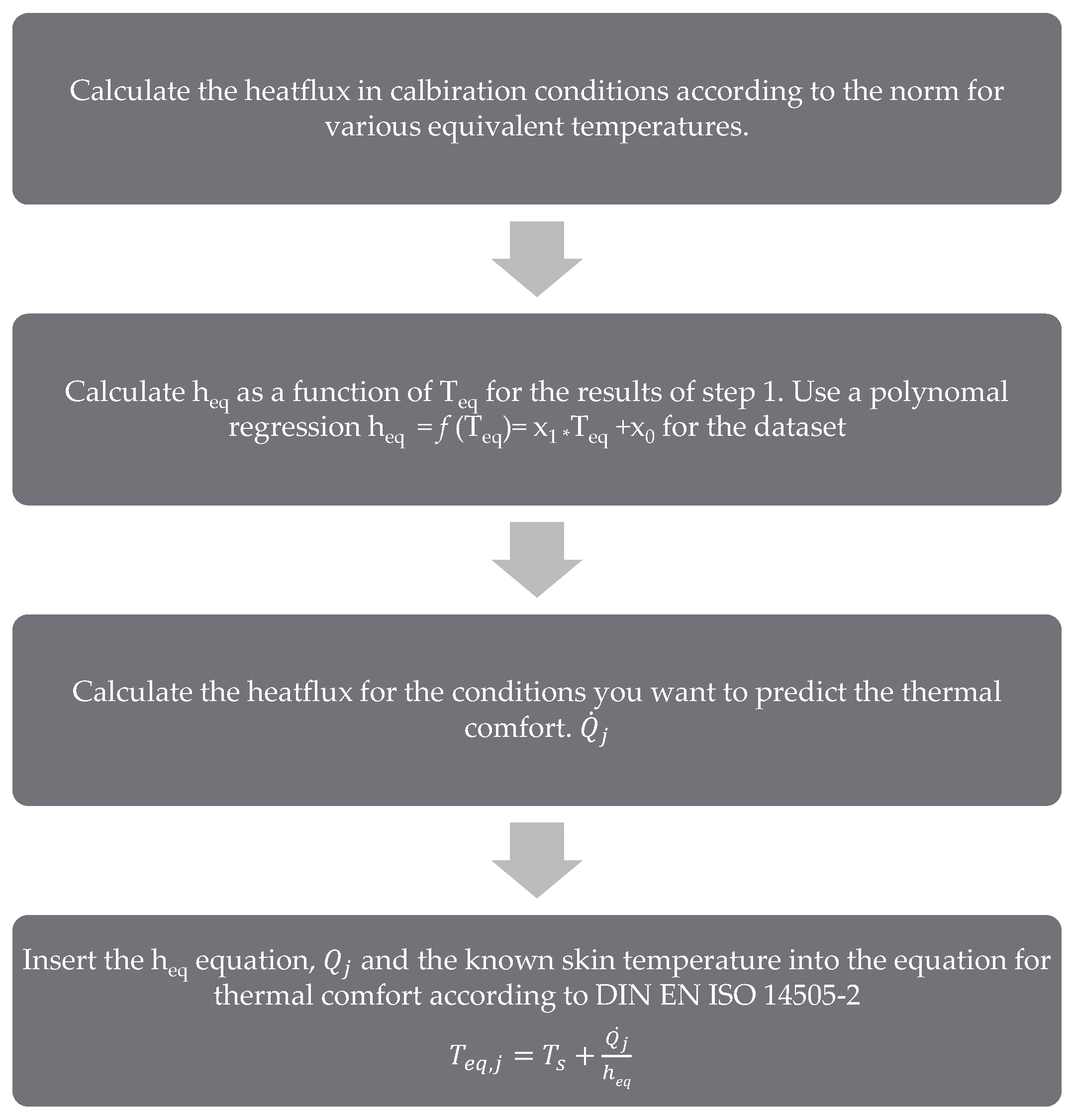
3. Simulation and Linearization of the Calibration Conditions
- Flow velocity 0.05 m/s;
- Temperature gradient < 0.4 K/m.
3.1. Turbulence Models
3.1.1. k-Epsilon Model
3.1.2. k-Omega Model
3.1.3. Laminar Model
3.1.4. Turbulent Viscosity
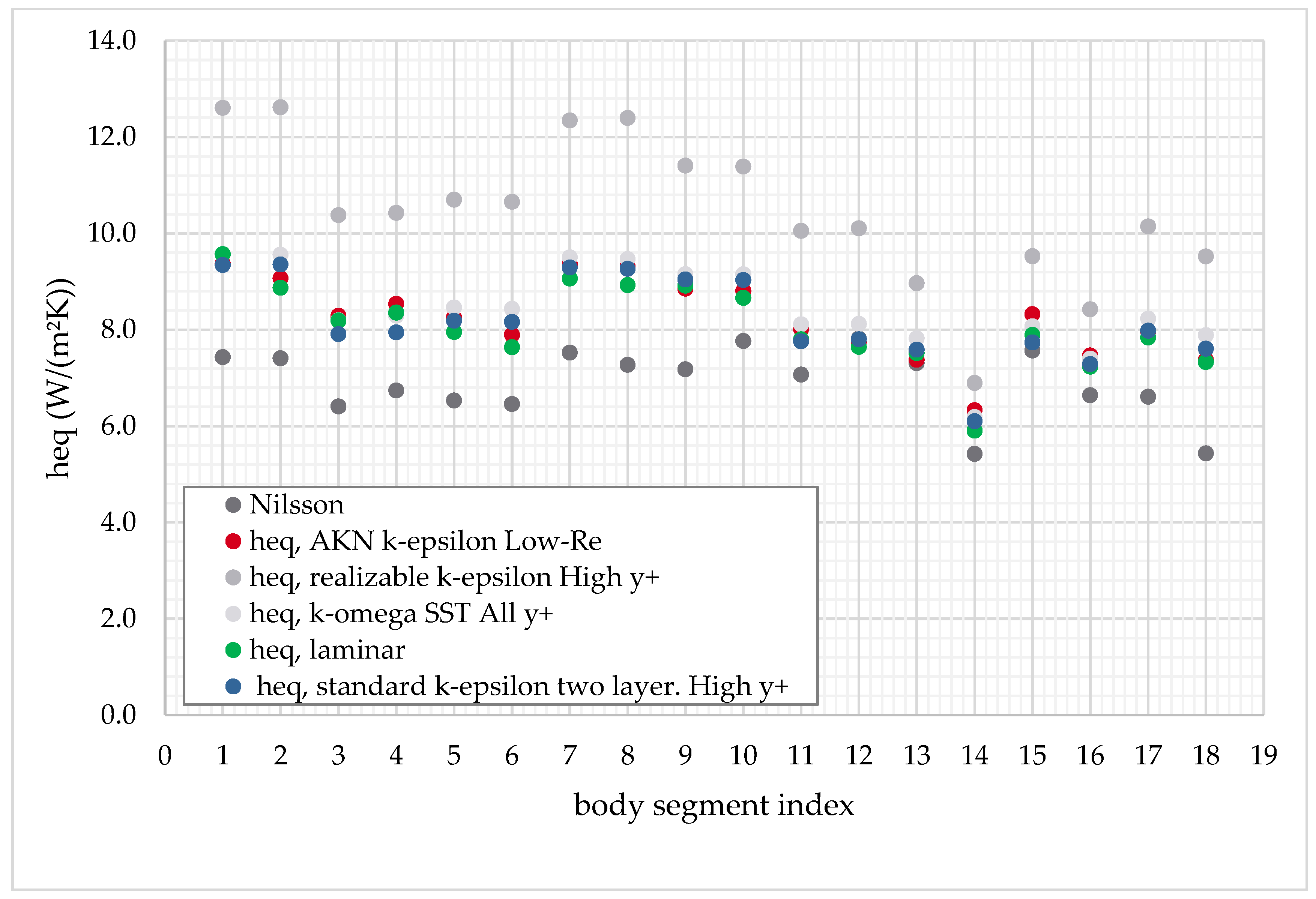
3.1.5. Model Comparison
−1*sqrt((${BoundaryHeatFlux}+${Ts}*${heq_x2}/min(${heq_x1},−1e-5) + pow((${heq_x2}-${Ts}*${heq_x1})
/(2*min(${heq_x2},−1e−5)),2))−(${heq_x2}−${Ts}*${heq_x2})/(2*min(${heq_x1},−1e−5))
4. Validation
4.1. Generic Cubic Room
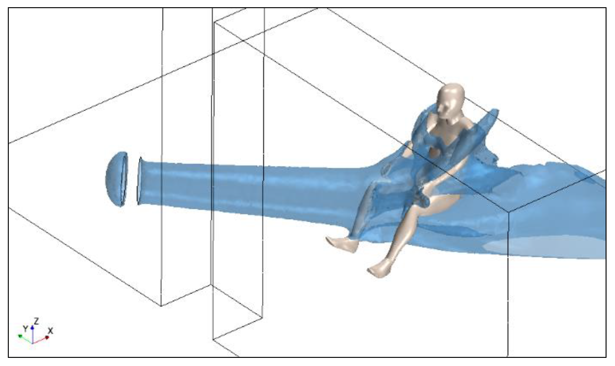
4.1.1. Model Setup
- A constant velocity inlet with 0.5 m/s in front of the manikin;
- An outlet behind the manikin;
- Left-hand side wall at 10 °C, right-hand side wall at 40 °C; the remaining walls are adiabatic.
4.1.2. Global Results
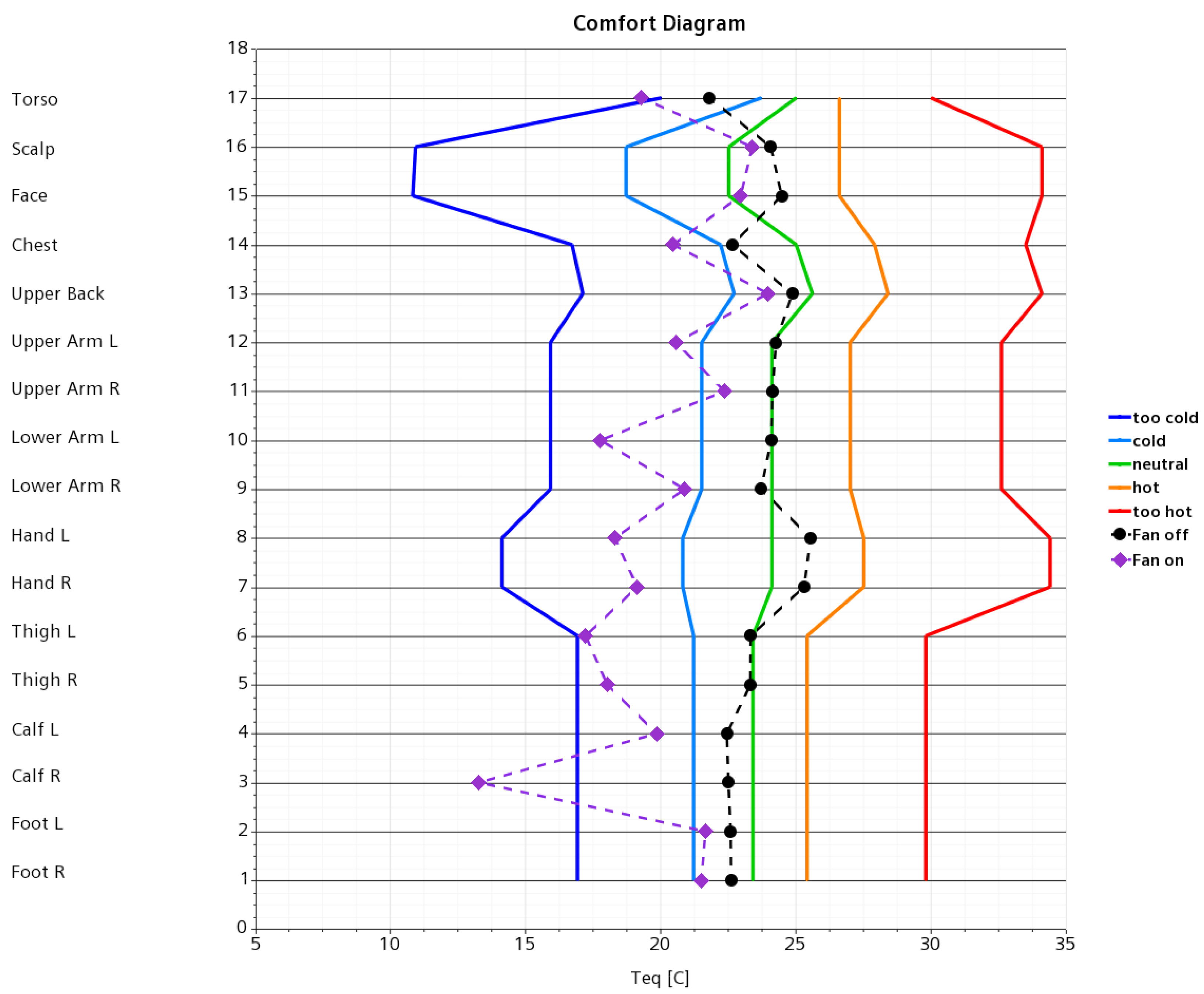
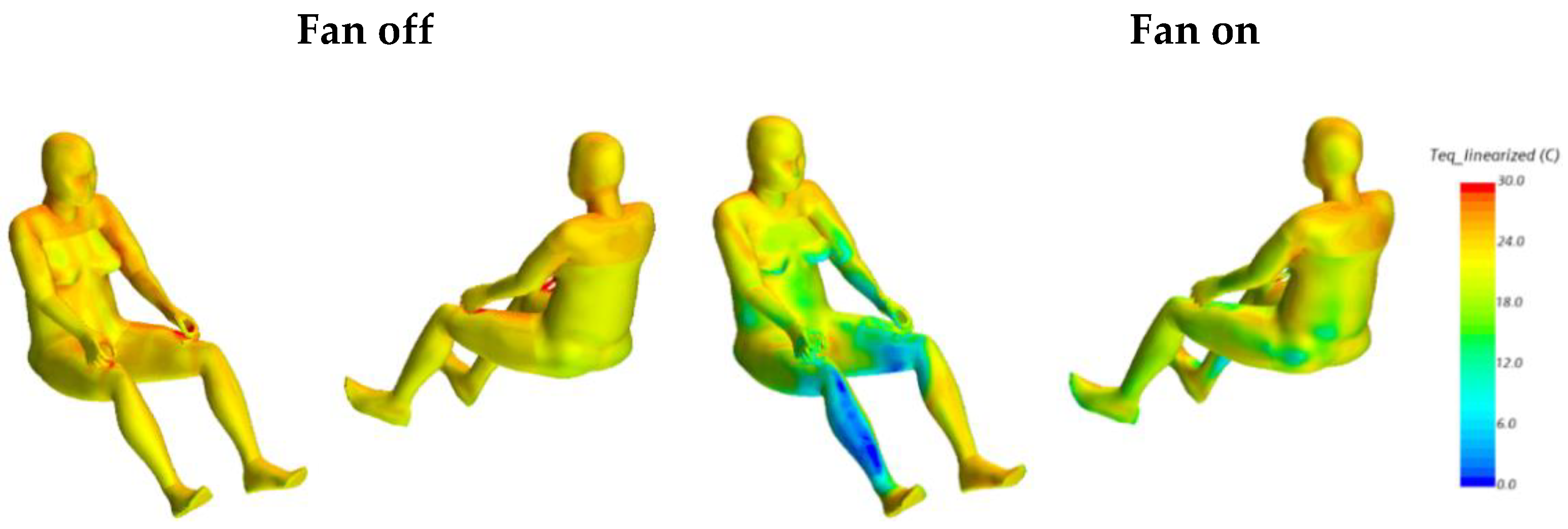
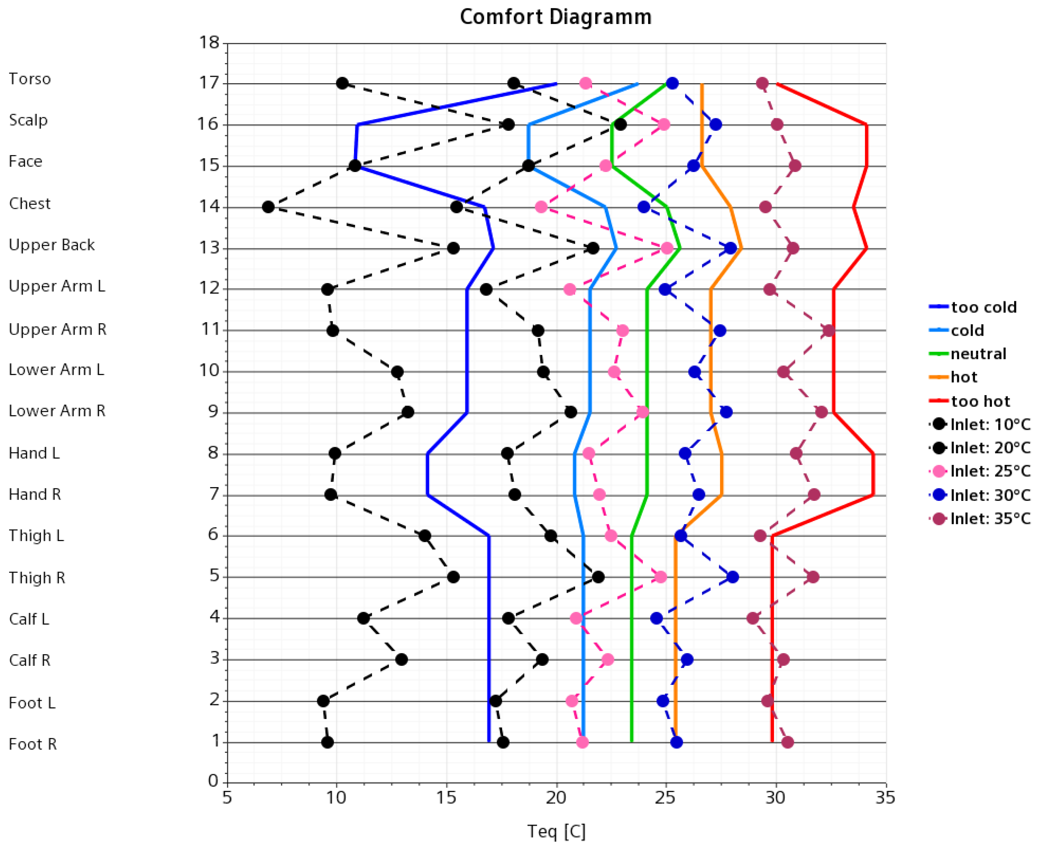
4.1.3. Local Thermal Comfort
4.2. Environmental Chamber
Setup
4.3. Global Results
Thermal Comfort
4.4. Computational Runtimes
5. Summary
6. Conclusions
Author Contributions
Funding
Conflicts of Interest
References
- Voelker, C.; Alsaad, H. Simulating the human body’s microclimate using automatic coupling of CFD and an advanced thermoregulation model. Indoor Air 2018, 28, 415–425. [Google Scholar] [CrossRef] [PubMed]
- Streblow, R. Thermal Sensation and Comfort Model for Inhomogeneous Indoor Environments. Dissertation’s Thesis, ON Energy Research Center, Tsukuba, Japan, 2010. [Google Scholar]
- ASHRAE-55. Refrigerating and Air-Conditioning Engineers: Thermal Environmental Conditions for Human Occupancy. Atlanta. 2004. Available online: https://www.ashrae.org/technical-resources/bookstore/standard-55-thermal-environmental-conditions-for-human-occupancy (accessed on 13 September 2021).
- Fanger, P.O.; Krieger, R.E. Thermal Comfort, Malabar; Bruel & Kjaer: Nærum, Denmark, 1982. [Google Scholar]
- DIN EN ISO 14505-2. Ergonomics of the Thermal Environment—Evaluation of Thermal Environment; Beuth: Berlin, Germany, 2004. [Google Scholar]
- Nilsson, H.; Holmér, I.; Bohm, M.; Norén, O. Equivalent Temperature and Thermal Sensation—Comparison with Subjective Responses; ATA: Bologna, Italy, 1997. [Google Scholar]
- Nilsson, H.O. Comfort Climate Evaluation with Thermal Manikin Methods and Computer Simulation Models, 3rd ed.; National Institute for Working Life: Stockholm, Sweden, 2004; p. 37. [Google Scholar]
- Fiala, D. Dynamic Simulation of Human Heat Transfer and Thermal Comfort, Leicester. Ph.D. Thesis, De Montfort University, Leicester, UK, 1998. [Google Scholar]
- Fiala, D.; Havenith, G.; Kampmann, B.; Jendritzky, G. UTCI-Fiala multinode model of human heat transfer and temperature regulation. Int. J. Biometerool. 2019, 56, 429–441. [Google Scholar] [CrossRef] [PubMed] [Green Version]
- Kingma, B. Human Thermoregulation: A Synergy between Physiology and Mathematical Modeling. Ph.D. Thesis, University of Maastricht, Maastricht, The Netherlands, 2021. [Google Scholar]
- Fiala, D.; Psikuta, A.; Jendritzky, G.; Paulke, S. Physiological modeling for technical, clinical and research applications. Front. Biosci. 2010, 2, 939–968. [Google Scholar] [CrossRef] [PubMed] [Green Version]
- Schwarz, M.; Krueger, M.W.; Busch, H.-J.; Benk, C.; Heilmann, C. Model-based assessment of tissue perfusion and tempera-ture in deep hypothermic patients. IEEE Trans. Biomed. Eng. 2010, 57, 1577–1586. [Google Scholar] [CrossRef] [PubMed]
- Xiaoyang, S.; Eckels, S.; Zhongquan, T. An improved thermal model of the human body. Hvac&r Res. 2011, 18, 323–338. [Google Scholar]
- Tang, Y.; He, Y.; Shao, H.; Ji, C. Assessment of comfortable clothing thermal resistance using a multi-scale human thermoregu-latory model. Int. J. Heat Mass Trans. 2016, 98, 568–583. [Google Scholar] [CrossRef]
- Dayi, L.; Qingjan, C. A two-dimensional model for calculating heat transfer in the human body in a transient and non-uniform thermal environment. Energy Build. 2016, 118, 114–122. [Google Scholar]
- Foda, E.; Sirén, K. A new approach using the Pierce two-node model for different body parts. Int. J. Biometeorol. 2010, 55, 519–532. [Google Scholar] [CrossRef]
- Kotb, H.; Khalil, E.E. Passengers’ Thermal Comfort in Wide-Body Aircraft Cabin. In AIAA Propulsion and Energy 2020 Forum; American Institute of Aeronautics and Astronautics: Reston, VA, USA, 2020. [Google Scholar]
- Sondes, I.; Zied, D. Numerical simulation and experimental validation of the ventilation system performance in a heated room. Air Qual. Atmos. Health 2020, 14, 171–179. [Google Scholar]
- Khatoon, S.; Kim, M.-H. Thermal Comfort in the Passenger Compartment Using a 3-D Numerical Analysis and Comparison with Fanger’s Comfort Models. Energies 2020, 13, 690. [Google Scholar] [CrossRef] [Green Version]
- Lange, P.; Schmeling, D.; Hörmann, H.J.; Volkmann, A. Comparison of local equivalent temperatures and subjective thermal comfort ratings with regard to passenger comfort in a train compartment. Mater. Sci. Eng. 2019, 609, 032042. [Google Scholar] [CrossRef]
- Schmidt, C.; Wölki, D.; Metzmacher, H.; van Treeck, C.A. Equivalent contact temperature (ECT) for personal comfort as-sessment as extension for ISO 14505-2, WINDSOR Rethinking Comfort Proceedings. Windsor 2018, 451–466. [Google Scholar]
- Sales, R.B.C.; Pereira, R.R.; Aguilar, M.T.P.; Cardoso, A.V. Thermal comfort of seats as visualized by infrared thermography. Appl. Ergon. 2017, 62, 142–149. [Google Scholar] [CrossRef]
- Cengiz, T.G.; Babalık, F.C. The effects of ramie blended car seat covers on thermal comfort during road trials. Int. J. Industr. Ergon. 2009, 39, 287–294. [Google Scholar] [CrossRef]
- Schmidt, C.; Praster, M.; Wölki, D.; Wolf, S.; van Treeck, C. Rechnerische und probandengestützte Untersuchung des Einflusses der Kontaktwärmeübertragung in Fahrzeugsitzen auf die thermische Behaglichkeit. FAT 2013, 261, 1–76. [Google Scholar]
- Taghinia, J.H.; Rahman, M.; Lu, X. Effects of different CFD modeling approaches and simplification of shape on prediction of flow field around manikin. Energy Build. 2018, 170, 47–60. [Google Scholar] [CrossRef]
- Yousaf, R.; Cook, M.; Wood, D.S.; Yang, T. CFD and PIV based investigation of indoor air flows dominated by buoyancy effects generated by human occupancy and equipment. In Proceedings of the 12th Conference of International Building Performance Simulation Association, Sydney, Australia, 14–16 November 2011. [Google Scholar]
- Lee, C.; Honma, H.; Melikov, A. An experimental study on convective heat transfer coefficient distribution on thermal manikin by air flow with various velocities and turbulence intensities. Trans. Arch. Inst. Japan 2003, 429, 25–31. [Google Scholar]
- Gao, S.; Ooka, R.; Oh, W. Formulation of human body heat transfer coefficient under various ambient temperature, air speed and direction based on experiments and CFD. Build. Environ. 2019, 160, 106168. [Google Scholar] [CrossRef]
- Yoshiichi Ozeki, H.; Oi, Y.; Ichikawa, A. Matsumoto, Evaluation of Equivalent Temperature in a Vehicle Cabin with a Numerical Thermal Manikin (Part 2): Evaluation of Thermal Environment and Equivalent Temperature in a Vehicle Cabin; SAE Technical Paper; SAE: Warrendale, PA, USA, 2019. [Google Scholar]
- Oi, H.; Ozeki, Y.; Suzuki, S.; Ichikawa, Y.; Matsumoto, A.; Takeo, F. Evaluation of Equivalent Temperature in a Vehicle Cabin with a Numerical Thermal Manikin (Part 1): Measurement of Equivalent Temperature in a Vehicle Cabin and Development of a Numerical Thermal Manikin; SAE: Warrendale, PA, USA, 2019. [Google Scholar]
- Morishita, M.; Uchida, T.; Mathur, G.D.; Kato, T.; Matsunaga, K. Evaluation of Thermal Environment in Vehicles for Occupant Comfort Using Equivalent Temperature of Thermal Manikin during Start-Stop Function with Energy Storage Evaporators. SAE Tech. Pap. Ser. 2018. [Google Scholar] [CrossRef]
- Bolineni, S. Development of Reduced Order Flow Responsive Convection Heat Transfer Models for Human Body Segments in Multiple Applications; Lehrstuhl für Energieeffizientes Bauen: Aachen, Germany, 2017. [Google Scholar]
- Rose, J. An approximate equation for the vapour-side heat-transfer coefficient for condensation on low-finned tubes. Int. J. Heat Mass Transf. 1994, 37, 865–875. [Google Scholar] [CrossRef]
- Ferziger, J.H.; Peric, M. Computational Methods for Fluid Dynamics; Springer: Berlin, Germany, 1997. [Google Scholar]
- Siemens, STARCCM+ Userguide, 2019. Available online: https://support.sw.siemens.com/ (accessed on 15 September 2020).
- Siegel, R.H. Thermal Radiation Heat Transfer; Hemisphere Publishing Co.: Boulder, CO, USA, 1992. [Google Scholar]
- Mathematische Nachbildung des Menschen—RAMSIS 3D-Softdummy, FAT-Bericht 135, Kaiserslautern, TECMAT GmbH; FAT-Bericht 135: Kaiserslautern, Germany, 1997.
- van Treeck, C.; Mitterhofer, M. Temperaturfeldberechnung aus Einer Particle Image Velocimetry (PIV) Messung Einer Natürlichen Auftriebsströmung; Bauphysik: Aachen, Germany, 2013. [Google Scholar]
- Tao, Z.; Cheng, Z.; Zhu, J.; Li, H. Effect of turbulence models on predicting convective heat transfer to hydrocarbon fuel at supercritical pressure. Chinese J. Aeronaut. 2016, 29, 1247–1261. [Google Scholar] [CrossRef] [Green Version]
- Wilcox, D.C. Turbulence Modeling for CFD; DCW Industries: La Canada, CA, USA, 1989. [Google Scholar]
- Menter, F.R. Two-equation eddy-viscosity turbulence modeling for engineering applications. AIAA J. 1994, 32, 1598–1605. [Google Scholar] [CrossRef] [Green Version]
- Atish, D.; Upender, G. A case study on human bio-heat transfer and thermal comfort within CFD. Build. Environ. 2015, 94, 122–130. [Google Scholar]
- Thomschke, C.; Bader, V.; Gubalke, A.; van Treeck, C. Bewertung der transienten thermischen Behaglichkeit in einer realen Fahr-zeugumgebung, Human-centred building(s). In Proceedings of the 5th German-Austrian IBPSA Conference, BauSIM 2014, International Building Performance Simulation Association, German Speaking Chapter, Mainz, Germany, 22–24 September 2014. [Google Scholar]
- Cook, M.; Yang, T. Cropper Thermal comfort in naturally ventilated classrooms: Application of coupled simulations models. In Proceedings of the Building Simulation, 12th Conference of International Building Performance Simulation Association, Sydney, Australia, 14–16 November 2011. [Google Scholar]


| Year of Publication | Realistic Manikin Geometry | Thermal Comfort Evaluation | Linearization of Parameters for Fast Calculation | Influence of the Flow Field on Thermal Comfort | Influence of the Turbulence Model on Thermal Comfort | Influence of the Radiation on Thermal Comfort | Variable Htc as Teq Function | |
|---|---|---|---|---|---|---|---|---|
| Taghinia [25] | 2018 | x | x | |||||
| Lee et al. [27] | 1991 | x | x | |||||
| Voelker et al. [1] | 2018 | x | x | x | ||||
| Gao et al. [28] | 2019 | x | x | x | ||||
| Ozeki et al. [29] | 2019 | x | x | x | x | |||
| Morishita et al. [31] | 2018 | x | x | x | x | |||
| Streblow et al. [2] | 2011 | x | x | x | x | |||
| Yousaf et al. [26] | 2011 | x | x |
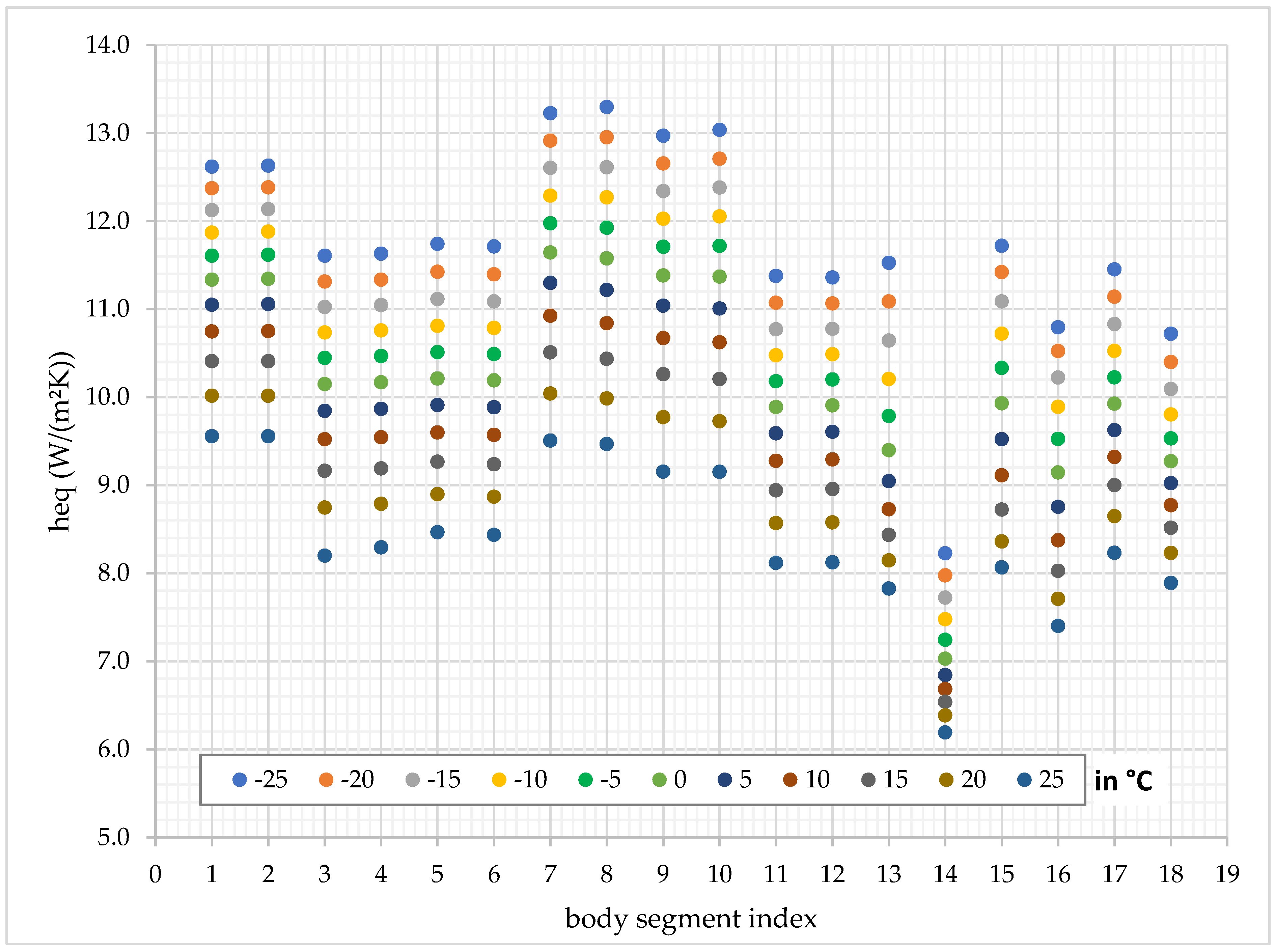
| Index | Letter | Name |
|---|---|---|
| 1 | a | Foot Right |
| 2 | b | Foot Left |
| 3 | c | Calf Right |
| 4 | d | Calf Left |
| 5 | e | Thigh Right |
| 6 | f | Thigh Left |
| 7 | g | Hand Right |
| 8 | h | Hand Left |
| 9 | i | Lower Arm Right |
| 10 | j | Lower Arm Left |
| 11 | k | Upper Arm Right |
| 12 | l | Upper Arm Left |
| 13 | m | Upper Back |
| 14 | n | Chest |
| 15 | o | Face |
| 16 | p | Scalp |
| 17 | q | Torso |
| 18 | x | Whole Body |
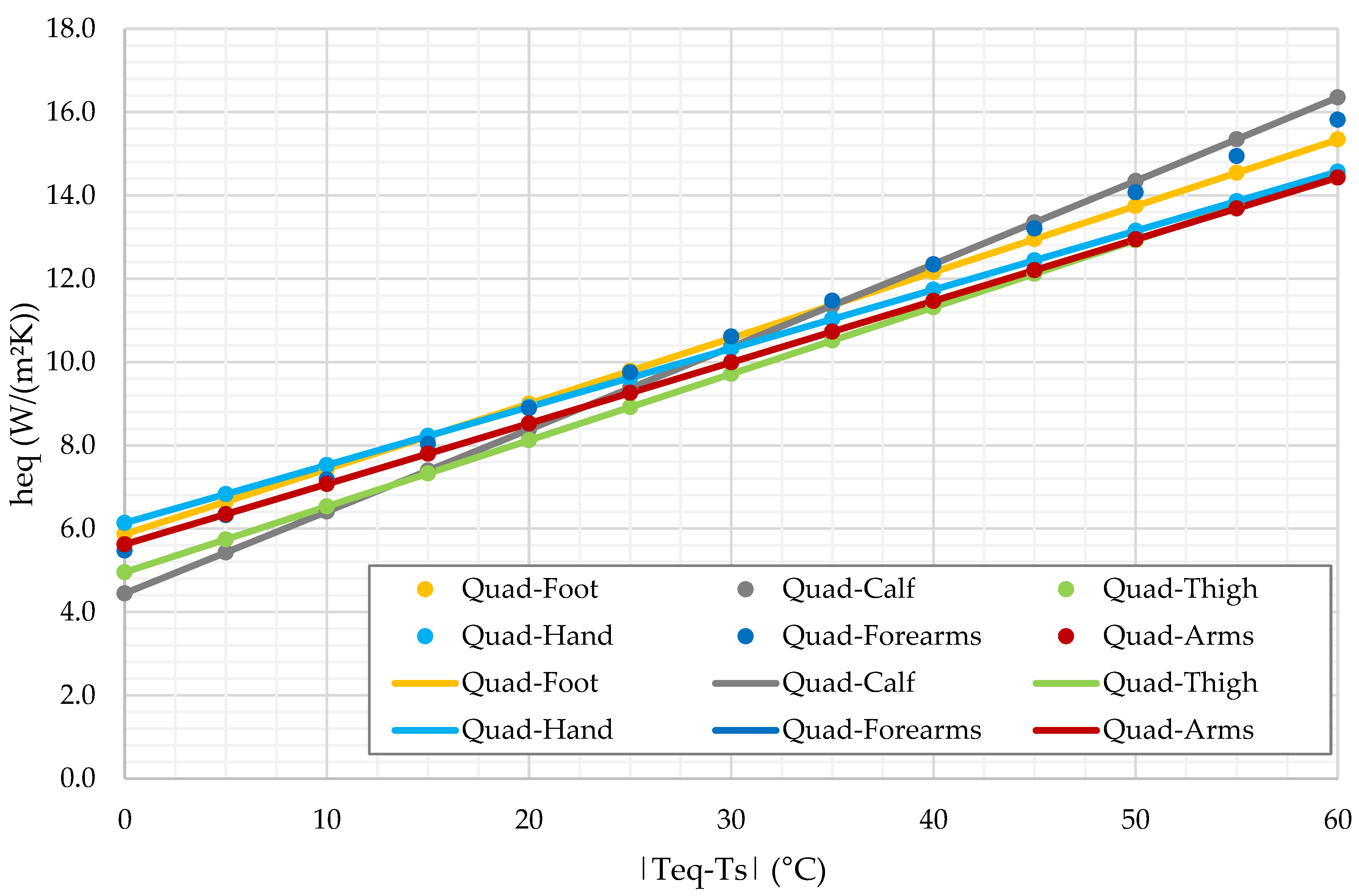
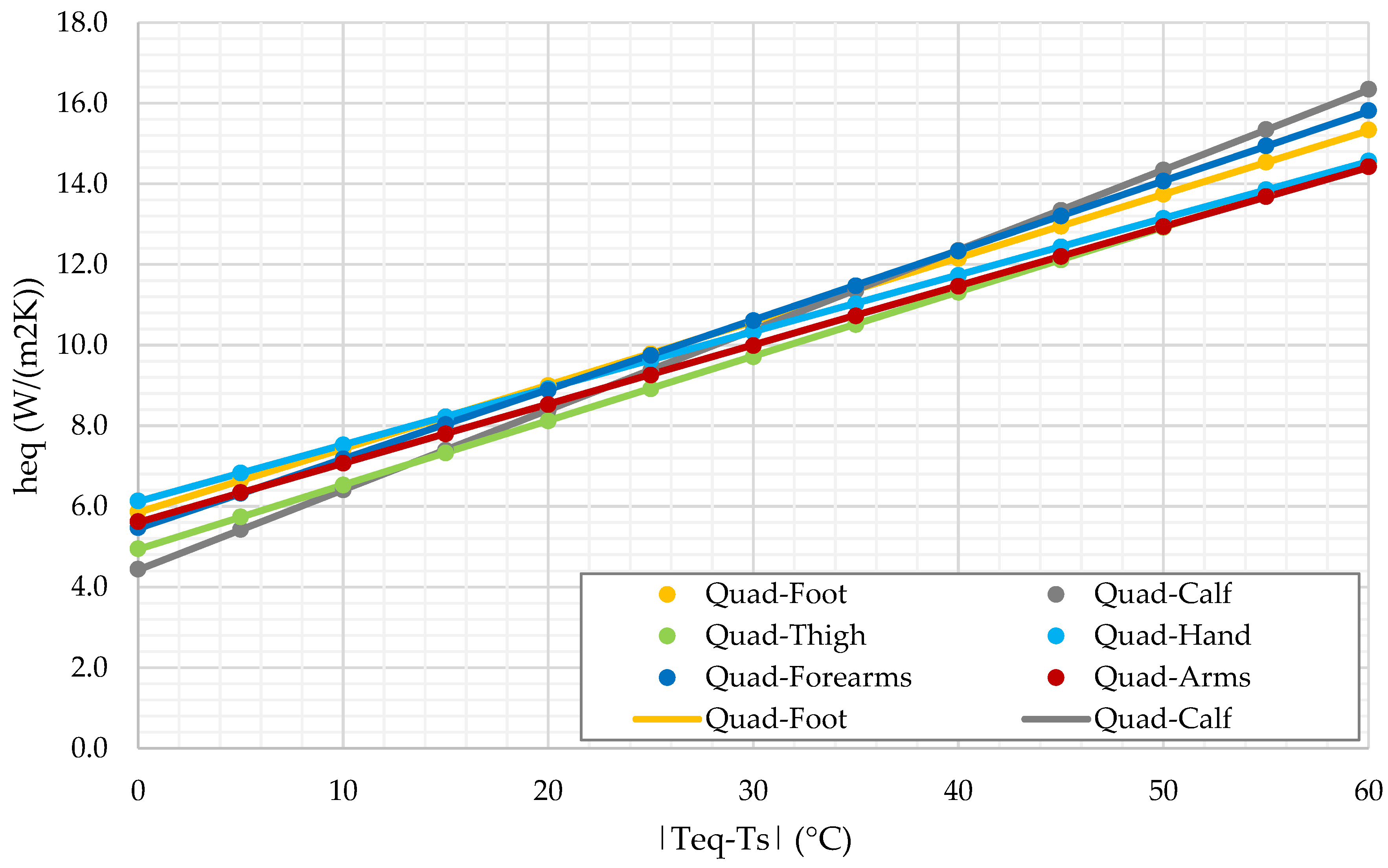
| Index j | Letter | Name | |||
|---|---|---|---|---|---|
| 1 | a | Feet | 3.28823 × 10⁻⁵ | 0.15589041 | 5.86819571 |
| 2 | b | Calf | 4.26080 × 10⁻⁵ | 0.19588617 | 4.44609867 |
| 3 | c | Thigh | 3.61242 × 10⁻⁵ | 0.15755566 | 4.95349670 |
| 4 | d | Hand | 3.05666 × 10⁻⁵ | 0.13870095 | 6.13626643 |
| 5 | e | Lower arms | 3.79767 × 10⁻⁵ | 0.14450724 | 5.62224012 |
| 6 | f | Upper arms | 3.79767 × 10⁻⁵ | 0.14450724 | 5.62224012 |
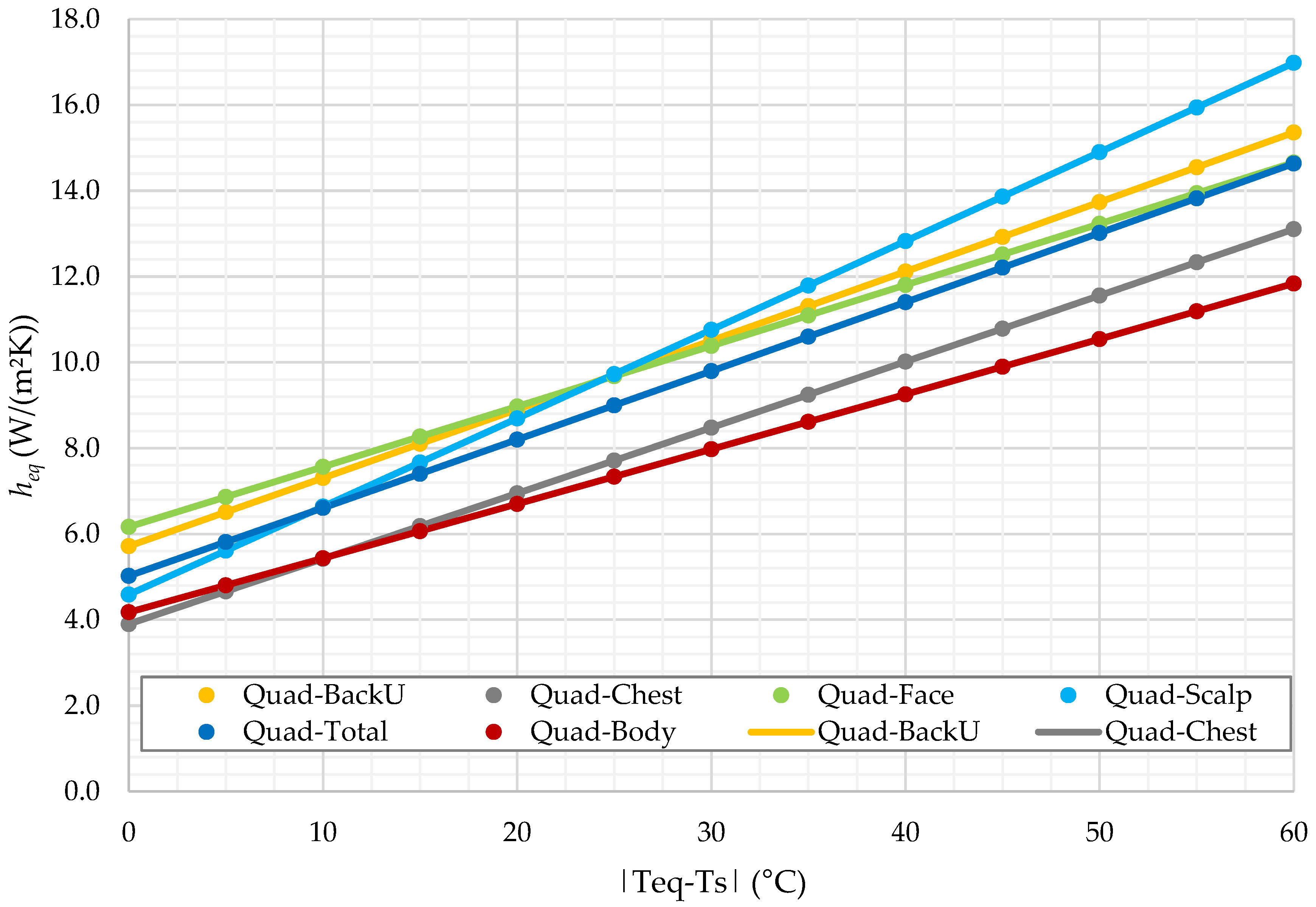
| 7 | g | Upper back | 3.61242 × 10⁻⁵ | 0.15855566 | 5.71649670 |
| 8 | h | Chest | 2.68616 × 10⁻⁵ | 0.15179780 | 3.90177959 |
| 9 | i | Face | 3.05666 × 10⁻⁵ | 0.13970095 | 6.16726643 |
| 10 | j | Scalp | 3.05666 × 10⁻⁵ | 0.20470095 | 4.58926643 |
| 11 | k | Total | 3.51979 × 10⁻⁵ | 0.15807988 | 5.02412499 |
| 12 | l | Body | 3.61242 × 10⁻⁵ | 0.12555566 | 4.17649670 |
| Index j | Name | ||
|---|---|---|---|
| 1 | Feet | 0.15786335 | 5.85011047 |
| 2 | Calf | 0.19844265 | 4.42266427 |
| 3 | Thigh | 0.15972311 | 4.9336284 |
| 4 | Hand | 0.14053494 | 6.1194548 |
| 5 | Lower arms | 0.17237992 | 5.45193974 |
| 6 | Upper arms | 0.14678584 | 5.60135294 |
| 7 | Upper back | 0.16072311 | 5.6966284 |
| 8 | Chest | 0.15340949 | 3.88700574 |
| 9 | Face | 0.14153494 | 6.1504548 |
| 10 | Scalp | 0.20653494 | 4.5724548 |
| 11 | Total | 0.16019175 | 5.00476614 |
| 12 | Body | 0.12772311 | 4.1566284 |
| Chamber size | 3.0 × 5.4 × 2.3 m (X, Y, Z) |
| Fan | Diameter: 300 mm Width: 100 mm Type: Fan Interface (approximately 200 m3/h) |
| Wall inlet | Type: Stagnation Inlet |
| Ceiling opening | Type: Pressure Outlet |
| Walls incl. ceiling | Adiabatic |
| Manikin | RAMSIS female, Lower fifth percentile T = 34 °C const. |
| Floor | T = 23 °C const. |
| Ambient temperature | Tamb = 23 °C |
| PMV with Teq | PPD with Teq (%) | DTS Final Value (Equation (27)) | PPD with DTS (%) | |
|---|---|---|---|---|
| Fan off | 0.38 | 8.1 | −0.19 | 5.7 |
| Fan on | −0.55 | 11.2 | −0.47 | 9.6 |
| Model | Fan | Runtime | PPD [%] |
|---|---|---|---|
| Linearized Teq Model | on | <1 h | 8 |
| off | <1 h | 11 | |
| DTS according to Cook et al. [44] | on | 34 h (average) | 6 |
| off | 18 h | 10 |
Publisher’s Note: MDPI stays neutral with regard to jurisdictional claims in published maps and institutional affiliations. |
© 2021 by the authors. Licensee MDPI, Basel, Switzerland. This article is an open access article distributed under the terms and conditions of the Creative Commons Attribution (CC BY) license (https://creativecommons.org/licenses/by/4.0/).
Share and Cite
Rommelfanger, C.; Fischer, L.; Frisch, J.; Van Treeck, C. Linearization of Thermal Equivalent Temperature Calculation for Fast Thermal Comfort Prediction. Energies 2021, 14, 5922. https://doi.org/10.3390/en14185922
Rommelfanger C, Fischer L, Frisch J, Van Treeck C. Linearization of Thermal Equivalent Temperature Calculation for Fast Thermal Comfort Prediction. Energies. 2021; 14(18):5922. https://doi.org/10.3390/en14185922
Chicago/Turabian StyleRommelfanger, Christian, Louis Fischer, Jérôme Frisch, and Christoph Van Treeck. 2021. "Linearization of Thermal Equivalent Temperature Calculation for Fast Thermal Comfort Prediction" Energies 14, no. 18: 5922. https://doi.org/10.3390/en14185922
APA StyleRommelfanger, C., Fischer, L., Frisch, J., & Van Treeck, C. (2021). Linearization of Thermal Equivalent Temperature Calculation for Fast Thermal Comfort Prediction. Energies, 14(18), 5922. https://doi.org/10.3390/en14185922