Observer Design for a Variable Moment of Inertia System

Abstract

Variable moment of inertia systems are common, and a popular laboratory system of this type is the “ball-and-beam”. Such systems are, however, nonlinear and often unstable. Efficient control requires full state information (or at least partial velocities), which are generally difficult to measure. That is why the design of state observers is a relevant problem. In this paper, a new design of an observer is proposed. This new nonlinear observer uses partial output injection and the circle criterion to ensure semiglobal stability. Moreover, we present a complete modeling of the system and systematic testing of the observer in comparison to a baseline in the form of a linear observer. The results show that the designed observer outperforms its linear counterpart and does not impede control.

1. Introduction

Systems with a varying moment of inertia are quite common in nature and in engineering, so interest in their properties is natural. One of the more common laboratory examples of such systems is the “ball-and-beam” (or “ball-on-beam”). Such systems remain ever popular [1,2,3]. This system is a nontrivial example of nonlinearity and the fourth order of dynamics with a mechanical realization. The control of such systems involving complications requires full state information, which cannot be directly measured and has to be estimated.

Methods for the control of “ball-and-beam” systems are various. Mazenc [4] used the direct Lyapunov method for the stability analysis. Sira [5] considered trajectory planning. Huang [6] used robust nonlinear control. Teel [7] designed a semiglobal output feedback. Ibanez [8] designed the control with the inverse Lyapunov approach. Lemos [9], Marton [10], Turker [11], Koo [12], and Naredo [13] used adaptive control. Xi [14] used nonlinear predictive control. Uran [15] used mechanism theory. Guo [16] designed a global stabilizer. Andreev [17] used matching control laws. Hauser [18] relied on approximate input–output linearization. Ortega [19] relied on interconnection and damping assignments. Krishna [20] used gain-scheduled PID. Banu Sundareswari [21] used intelligent PID tuning. Recently, fuzzy control was also applied to control the ball-and-beam system in the works of Chang [22], Asadi [23], and Minh [24]. Aziz et al. in 2013 also presented some methods for stabilization of the ball on a two-dimensional beam [25]. State observers were presented for this system by Joo [26,27].

In this paper, we consider methods of state estimation for the system (1). Both nonlinear and linear observer designs are presented, and their performance is compared and illustrated with simulations. Our nonlinear observer design is novel, as it reformulates its error dynamics as a Lurie system. Lurie systems are a type of feedback system with linear dynamics and nonlinear, static (but potentially time-varying) feedback. Lurie systems enjoy a well-grounded theory of stability [28], but are still a thriving field of study [29,30,31,32,33].

The main contributions of the paper are as follows:

• A systematic model design of the “ball-and-beam” system;
• The design of a nonlinear observer with a specific structure and stability proven in a novel way;
• A systematic analysis and comparison with a typical linear observer.

The comparisons are made both in open-loop and closed-loop (with a linear controller). The observer design for the ball-and-beam system was also considered in [26,27].

The rest of the paper is organized as follows. First, we present the ball-on-beam variable moment of inertia system; we formulate its equations and present the method by which they were obtained and how to obtain the system parameters. Then, we describe the methods that we used to illustrate our contribution. First, we show how a linear, reference observer can be designed. Then, we present our proposed structure and prove its stability. Finally, we explain which control structures were used to show how the observer operates. Then, we move to the simulation experiments, where we show how observers operate both independently and as a part of the control system. The paper ends with a discussion and conclusions.

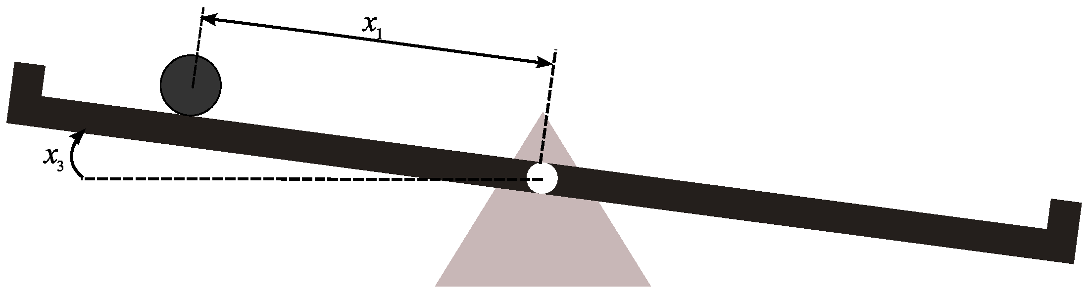
2. Ball-on-Beam Variable Moment of Inertia System

A schematic illustration of the ball-and-beam system is depicted in Figure 1. This and similar systems were considered among others in [34,35] Typically, one is interested in the stabilization of the position of the ball at the middle of the beam, while the beam is in a position parallel to the ground. It is easily verifiable that the equilibrium considered is unstable. Many different stabilization techniques can be applied to solve this problem. One of them is static linear state feedback (i.e., it can be a solution to the linear quadratic problem for the system’s linearization).

However, usually, only positions ($x_1$ and $x_3$) can be measured, so to apply the state feedback controller, one needs to know the values of the velocities. A very good way to obtain them is the state observer.

The mathematical model of the system consists of the following equations:

$$\begin{array}{ccc}\hfill {\dot{x}}_1& =& x_2\hfill \\ \hfill {\dot{x}}_2& =& a_{1}sin{x}_3+a_2{x}_1{x}_4^2\hfill \\ \hfill {\dot{x}}_3& =& x_4\hfill \\ \hfill {\dot{x}}_4& =& \frac{g{x}_{1}cos{x}_3-b_{2}sin{x}_3}{b_1+x_1^2}+\frac{b_{3}u}{b_1+x_1^2}\hfill \end{array}$$

(1)

where $x_1$ is the ball’s position, $x_2$ is the ball’s velocity, $x_3$ is the beam’s angle, and $x_4$ is the beam’s angular velocity. The driving torque is applied to the beam’s joint and is represented as a control signal u. Such a model is convenient for implementation, and its determination is described in the following section.

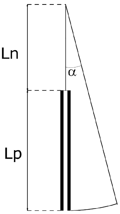
2.1. Determination of the Physical Model

A good method to determine models of mechanical systems is the Euler–Lagrange formalism, which was used in [34]. A more advanced approach to modeling was used in [11,36,37,38,39]. In order to create the model, its parameters have to be considered.

The system depicted in Figure 1 consists of a rotating beam and a ball rolling on it. The system has the following physical parameters:

• $J_{beam}$—beam moment of inertia (kg·m ${}^2$);
• m—ball weight (kg);
• r—ball radius (m);
• $L_p$—beam length (m).

We assumed that we can control the torque of the beam M. For the purpose of modeling, we made the following assumptions:

(1)

The ball does not slide on the beam (it only rolls);

(2)

The angle of the beam $\left|\alpha \right|\le {\alpha }_{max}$;

(3)

The friction is negligible;

(4)

The ball is perfectly round and homogenous;

(5)

The ball does not rebound from limiters;

(6)

The ball does not lose contact with the beam;

(7)

The beam is perfectly symmetric and flat.

There are many approaches in the literature to obtain the model’s equation. To derive the state equations for this system, we used the Euler–Lagrange formalism [40]:

$$\frac{d}{dt}\left(\frac{\partial \mathcal{L}}{\partial {\dot{x}}_i}\right)-\frac{\partial \mathcal{L}}{\partial x_i}+\frac{1}{2}\frac{\partial P}{\partial {\dot{x}}_i}=F_i$$

(2)

where $\mathcal{L}$ is the Lagrangian, P is the Rayleigh loss function, $F_i$ are the forces having an influence on the system, and $x_i$ are the generalized coordinates. The Lagrangian takes the form:

$$\mathcal{L}=E_k-E_p$$

(3)

where:

$E_p$—the potential energy of the ball, given by the equation:

$$E_p=mgh$$

(4)

$E_k$—the kinetic energy of the ball-and-beam given by the equation:

$$E_k=\frac{1}{2}m{x}_2^2+\frac{1}{2}{J}_{ball}{\omega }^2+\frac{1}{2}\left(J_{beam}+J_{ball-0}\right)x_4^2$$

(5)

with $\omega$ the angular velocity of the ball.

The Rayleigh loss function in this case is very simple, as it only relates to the rolling friction of the ball:

$$P=b{x}_1^2$$

(6)

with b the friction coefficient. $F_i$ is the torque applied to the axis of the beam, and we denote it as M.

Remark 1.

In Equation (4), we made an assumption about the ball’s vertical position h. We also assumed that $h=0$ on the beam axis level. It would be more common to assume $h=0$ at the point where the ball’s vertical position is minimal. However, in this case, h would be dependent on other system parameters: the beam length l and the max beam angle ${\alpha }_{max}$. This would make the equations more difficult to compute and analyze. Nevertheless, it has to be mentioned that this assumption allows the potential energy of the ball to be negative, and as a result, the sum of all energies in the system can also be negative.

After a simple trigonometric operation, the following expression for the potential energy can be written as:

$$E_p=mg\left(x_{1}sin{x}_3+rcos{x}_3\right)$$

(7)

In the kinetic energy Equation (5), the moment of inertia of the ball with respect to the beam junction and the moment of inertia of the ball in its body center can be expressed as:

$$\begin{array}{cc}\hfill J_{ball-0}=& \frac{2}{5}m{r}^2+m\left(r^2+x_1^2\right)\hfill \end{array}$$

(8)

$$\begin{array}{cc}\hfill J_{ball}=& \frac{2}{5}m{r}^2\hfill \end{array}$$

(9)

The angular rate of the ball is simply related to its linear velocity:

$$\omega =\frac{x_2}{r}$$

(10)

Evaluating the Lagrange equation leads to the formulation of the following differential equations:

$$\begin{array}{cc}\hfill 0=& \frac{7}{5}m{\dot{x}}_2+mgsin{x}_3-m{x}_1{x}_4^2+b{x}_2\hfill \\ \hfill M=& {\dot{x}}_4\left(J_{beam}+\frac{7}{5}m{r}^2+m{x}_1^2\right)-mg\left(rsin{x}_3-x_{1}cos{x}_3\right)\hfill \end{array}$$

(11)

After substituting (3) into (2), we obtain the following state equations (with the classical choice of physical symbols for generalized coordinates):

$$\begin{array}{ccc}\hfill {\dot{x}}_1& =& x_2\hfill \\ \hfill {\dot{x}}_2& =& \frac{5}{7}\left(-gsin{x}_3+x_1{x}_4^2-\frac{b}{m}{x}_2\right)\hfill \\ \hfill {\dot{x}}_3& =& x_4\hfill \\ \hfill {\dot{x}}_4& =& \frac{mg(rsin{x}_3-x_{1}cos{x}_3)+M}{(J_{beam}+m(\frac{7}{5}{r}^2+x_1^2))}\hfill \end{array}$$

(12)

In order to simplify the implementation of the model, it can be transformed to the form of (1) with $u=M$. The parameters from (12) and (1) along with the explicit formulas are presented in

Table 1. Physical model parameters are inconvenient to use when implementing models in software environments. That is why for our implementation, we preferred the form with nonphysical, precomputed parameters. For convenience, this table includes both physical and precomputed parameters along with explicit formulas.

Physical Parameters		Computational Parameters
m	0.208 kg	$a_1=\frac{5}{7}g$	7.007
r	0.018 m	$a_2=\frac{5}{7}$	0.7143
$L_p$	0.4 m	$b_1=\frac{J_{beam}}{m}+\frac{7}{5}{r}^2$	0.0365
$J_{beam}$	0.0075 kg·m ${}^2$	$b_2=g·r$	0.1814
g	9.81 $\frac{\mathrm{m}}{{\mathrm{s}}^2}$	$b_3=\frac{1}{m}$	4.8077
b	0

.

2.2. Model Parameters

The ball mass m and radius r, along with the beam’s length $L_p$ can be computed directly. To compute the beam’s inertia moment, we need to compute its mass $m_b$ as well. Afterwards, we performed the following experiment: The beam was hung on a thread with length $L_n$ (see Figure 2). Afterwards, the beam was made to have small oscillations (we assumed in the $\alpha$ range $sin\alpha =\alpha$). The period of this oscillation T was measured.

Afterwards, we used an equation for the physical pendulum:

$$T=2\pi \sqrt{\frac{J_{beam}}{m_{b}gd}}$$

(13)

where d is the distance between the beam’s center of gravity and the point where the thread is attached, in our case:

$$d=\frac{1}{2}{L}_p+L_n$$

(14)

where: $L_p$—length of the beam, $L_n$—length of the thread.

After substituting (14), Equation (13) can be transformed to the following:

$$J_{beam}=m_{b}g\left(\frac{1}{2}{L}_p+L_n\right){\left(\frac{T}{2\pi }\right)}^2$$

(15)

Factors on the right side, such as the weight, the length of the thread and the beam, and the pendulum’s period, are easy to measure and allow estimating the beam’s inertia moment. Finally, the friction coefficient was assumed to be negligible.

3. Methods

In this section, we cover the methods of state estimation that were considered in this paper. First, we present the design of the linearized observer and determine the Jacobi matrix, the observability, and the observer gain. Then, we move to the new proposed observer structure and prove its semiglobal stability. Finally, we present the control structures that we considered to analyze the observers.

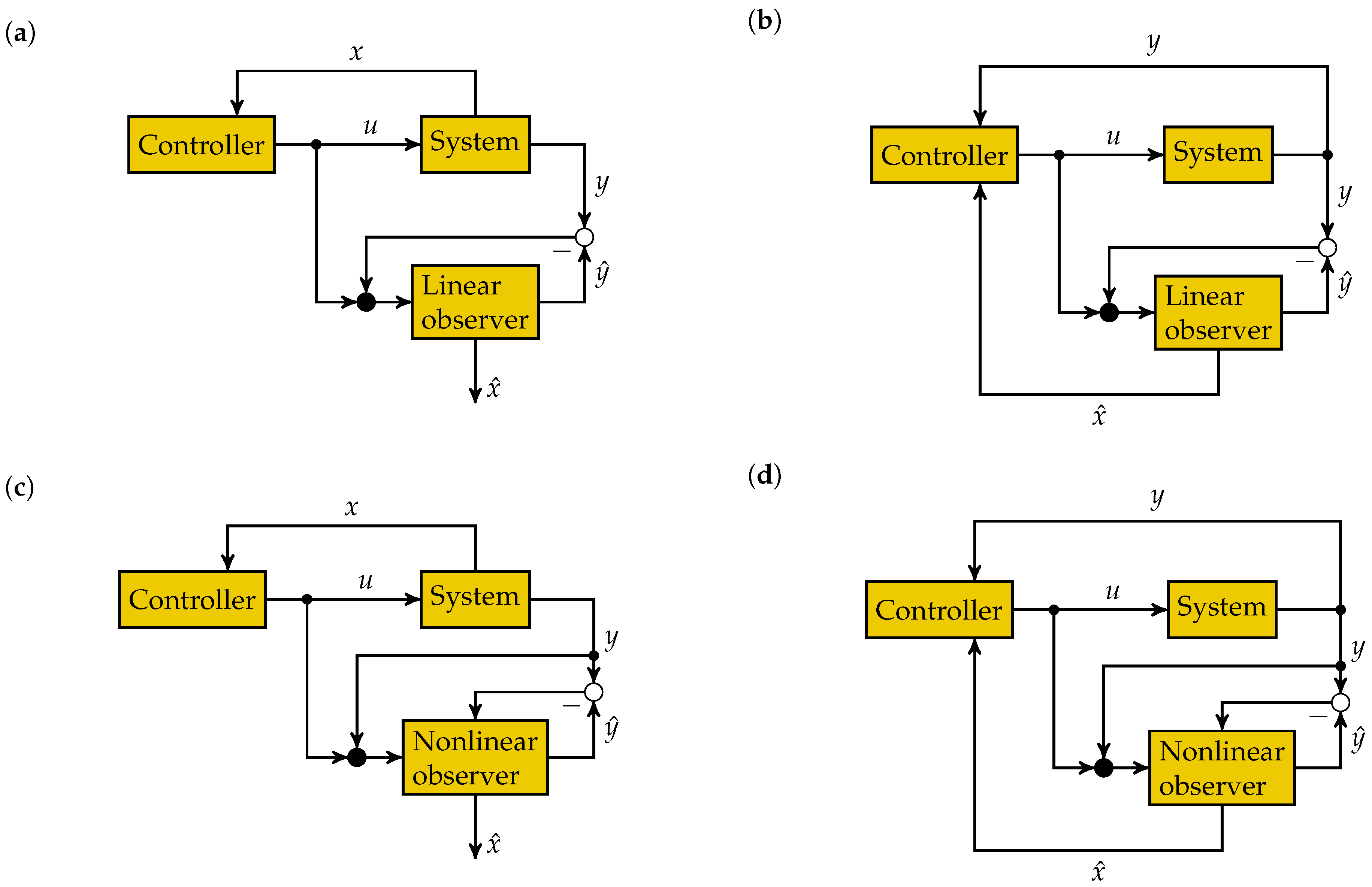
3.1. Linear Observer Design

First, we present the observer for a linearized system. We present it first because it can be seen that for the system (1), the Jacobi matrix takes the form:

$$J\left(x\right)=\left[\begin{array}{cccc}0& 1& 0& 0\\ a_2{x_4}^2& 0& a_{1}cos\left(x_3\right)& 2a_2{x}_1{x}_4\\ 0& 0& 0& 1\\ f_1\left(x\right)& 0& f_2\left(x\right)& 0\end{array}\right]$$

(16)

where:

$$f_1\left(x\right)=\frac{gcos\left(x_3\right)}{b_1+{x_1}^2}-2\frac{\left(g{x}_{1}cos\left(x_3\right)-b_{2}sin\left(x_3\right)\right)x_1}{{\left(b_1+{x_1}^2\right)}^2}$$

$$f_2\left(x\right)=\frac{-g{x}_{1}sin\left(x_3\right)-b_{2}cos\left(x_3\right)}{b_1+{x_1}^2}$$

This form of the Jacobi matrix is coupled with the system output:

$$y=\left[\begin{array}{cccc}1& 0& 0& 0\\ 0& 0& 1& 0\end{array}\right]x=Cx$$

(17)

allowing the use of the strongest observability criteria for the nonlinear systems. The criteria (see for example [41] or compare with the analogous result for controllability [42]) state that the nonlinear system is locally observable at the point $x^{\ast }$ if the pair $\left(C;J\left(x^{\ast }\right)\right)$ is observable. For the considered system, we can verify that the observability matrix (see for example [43]) takes the form:

$$Q=\left[\begin{array}{c}C\\ CJ\left(x^{\ast }\right)\end{array}\right]=\left[\begin{array}{cccc}1& 0& 0& 0\\ 0& 0& 1& 0\\ 0& 1& 0& 0\\ 0& 0& 0& 1\end{array}\right]$$

Therefore, Q is independent of $x^{\ast }$ and nonsingular. This means that the system (1) with (17) is locally observable everywhere. Knowing the Jacobi matrix, we can compute linear approximation of system (1) near the 0 equilibrium, resulting in the linear system:

$$\mathsf{∆}\dot{x}=A\mathsf{∆}x+Bu$$

where $A=J\left(0\right)$ and $B=\frac{\partial }{\partial u}F(x,u)$ with $F(x,u)$ being the right side of (1) and $\mathsf{∆}x$ is a deviation from 0 equilibrium. Using such a system, one can propose a linear Luenberger observer:

$$\dot{\widehat{x}}=A\widehat{x}+Bu+G_1(y-C\widehat{x})$$

(18)

For this observer, the gain matrix $G_1$ was chosen in such a way that eigenvalues of the matrix $A-G_{1}C$ were real in the interval range $[-21,-20]$. Such a choice of the gain is not perfect, and the search for the optimal one is advised. Such problems were considered among others in [44,45]. The observer gain was computed using the place method from the MATLAB^® Control Toolbox™ [46] (or equivalently using the Python Control Systems Library [47]; both implement the algorithm by Kautsky et al. [48]) and has the form:

$$G_1=\left[\begin{array}{cc}41& 0\\ 420& 7.007\\ 0& 41\\ 268.496& 415.033\end{array}\right]$$

(19)

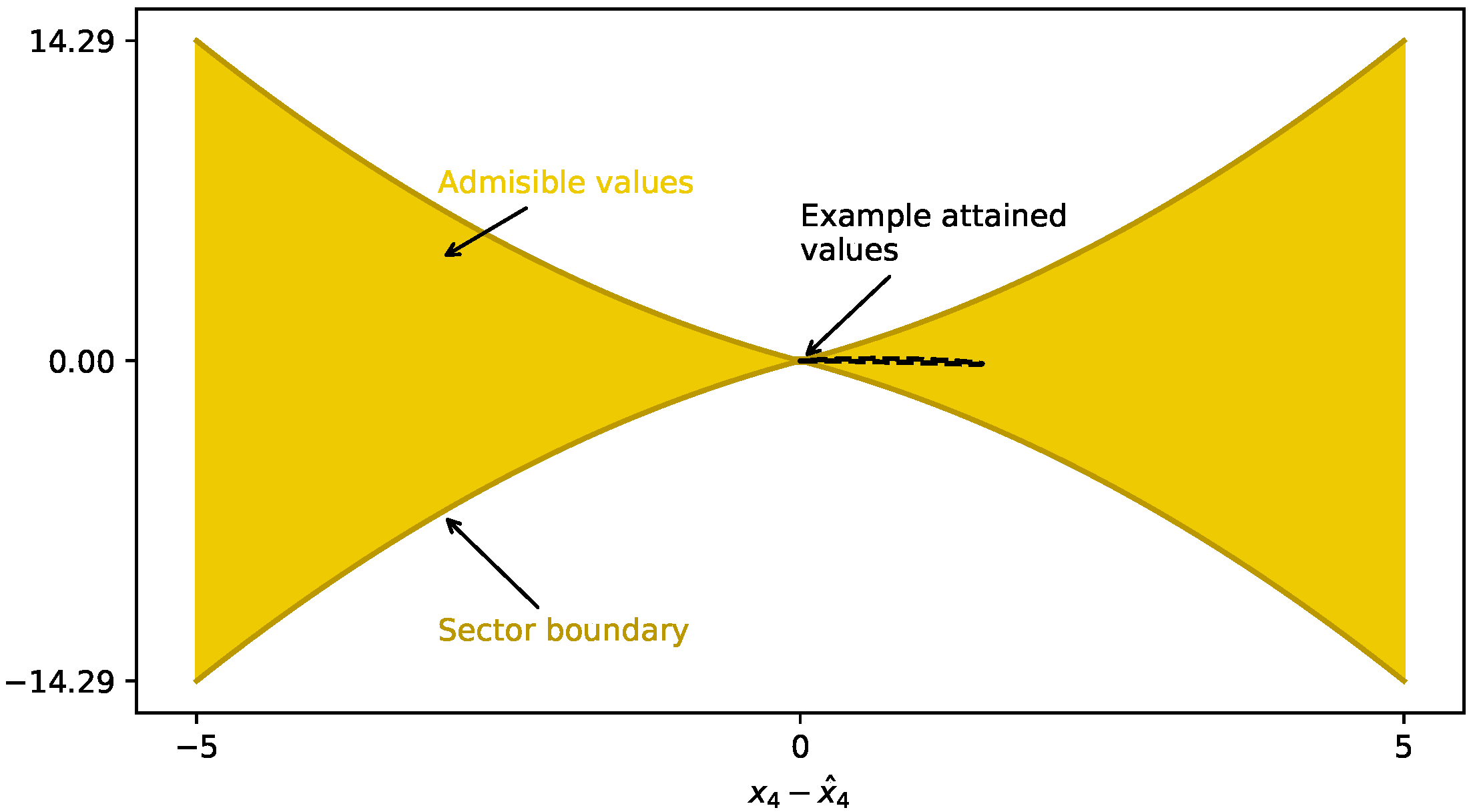
3.2. Nonlinear Observer Design

For the design of the nonlinear observer for the system (1), one should see that the right side of (1) has the following structural property:

$$F(x,u)=Lx+F_1(x_1,x_3)+F_2(x_1,x_4)+F_3\left(x_1\right)u$$

where L is in block-diagonal Frobenius form (see [49]):

$$L=\left[\begin{array}{cccc}0& 1& 0& 0\\ 0& 0& 0& 0\\ 0& 0& 0& 1\\ 0& 0& 0& 0\end{array}\right]$$

Using this form, one can propose a nonlinear observer:

$$\dot{\widehat{x}}=L\widehat{x}+G_2(y-C\widehat{x})+F_1(x_1,x_3)+F_2(x_1,{\widehat{x}}_4)+F_3\left(x_1\right)u$$

(20)

This is similar approach to the so-called output injection observers, where it is intended to cancel as many as possible nonlinear terms in the error equation.

The dynamics of the error for such an observer has (after simple transformations and setting ${\widehat{x}}_4=x_4-e_4$) the following form:

$$\dot{e}=(L-G_{2}C)e-bf(c^{\mathsf{T}}e,t)$$

(21)

where:

$$b=\left[\begin{array}{c}0\\ 1\\ 0\\ 0\end{array}\right]c=\left[\begin{array}{c}0\\ 0\\ 0\\ 1\end{array}\right]$$

and:

$$f(v,t)=a_2{x}_1\left(t\right)(v^2-2x_4\left(t\right)v)$$

(22)

Therefore, the dynamics of the error is a linear system with one scalar, time-varying nonlinearity (nonautonomous Lurie system [28]).

Remark 2.

It should be noted that because $x_3$ is bounded due to the assumptions, $x_1$ is bounded because of the finite length of the beam, and the control torque is bounded; for practical reasons, also $x_2$ and $x_4$ are bounded, and those bounds can either be computed through simulations or estimated analytically. In other words, one can consider $x_1$ and $x_4$ as bounded time-varying parameters, so (22) is a quadratic function with time-varying parameters. In Figure 3, one can see the sector in which the values of (22) are contained: the upper bound of the sector is ${sup}_{x_1,x_2}f(v,t)$, and the lower bound is ${inf}_{x_1,x_2}f(v,t)$.

The system (21) is in the form that allows the application of the circle criterion (see [28,50]). In Figure 3, one can see that the global asymptotic stability of (21) is impossible, because the sector containing the nonlinear function (22) grows quadratically.

For such a system, we can compute the transfer function:

$$G\left(s\right)=c^{\mathsf{T}}{((L-G_{2}C)-sI)}^{-1}b$$

which for the appropriate choice of $G_2$ and setting the eigenvalues of the matrix $A-G_{2}C$ as real and contained in the interval $[-21,-20]$, allows achieving the modulus of the transfer function with a ${10}^{-17}$ order of magnitude. This gain, computed similarly to the previous one, has the form:

$$G_2=\left[\begin{array}{cc}41& 0\\ 420& 0\\ 0& 41\\ 0& 420\end{array}\right]$$

(23)

For such a gain, one can see that the appropriate frequency inequality is fulfilled (see [28]):

$$I+\frac{1}{2}(k_1+k_2)(G\left(j\omega \right)+G(-j\omega ))+k_1{k}_2{\left|G\left(j\omega \right)\right|}^2\ge 0$$

where $k_1,k_2$ are chosen so that $k_{1}v+\epsilon \le f(v,t)\le k_{2}v-\epsilon$ for $v\in [e_{4min},e_{4max}]$ and some $\epsilon >0$. This allows solving the appropriate Lyapunov equation and finding the quadratic form, that is the Lyapunov functional for (21) and semipositive definite, giving the basin of attraction consisting of all the possible initial errors (because of the original system state constraints).

Such a situation is the example of the so-called semiglobal stability property. Regarding the observer design, by the choice of the parameter (in our case $G_2$), one can achieve any desired finite basin of attraction.

3.3. Considered Control System

As stated earlier, our idea for the observer design was to estimate the velocities (linear of the ball and angular of the beam) that cannot be implemented directly. Then, we would have the full state information that we could use to construct the feedback. As a simple solution to the feedback problem (as it is not the main focus of the paper), we used a linear feedback control, designed to set the eigenvalues of the closed-loop system as linearized around the equilibrium and as real in the interval $[-3,-4]$. This can be obtained using the place method mentioned earlier. One gain realizing this postulate has the form:

$$K=\left[\begin{array}{cccc}2.197& 0.183& 0.518& 0.106\end{array}\right]$$

(24)

To keep the realism in the controller, we introduced saturation, making the control limited as $\left|u\right|<5$. It is important to notice that this is not a globally stabilizing controller. That is why large transitional errors can move it outside of the basin of attraction and cause system instability. Moreover, it should be noted that, in general, for nonlinear systems, there is no separation property. Therefore, the globally stable observer and globally stable controller might not result in a globally stable system. That is why we compared our observers both inside and outside of the control loop.

To test the observers, we used this controller in two ways. First, we close a feedback loop with the system state and introduced the observer just as a state estimator. Such a structure is presented in Figure 4a,c.

The second structure that we wanted to use was the implementation of the observer in the control loop. In this case, we used the position (linear of the ball and angular of the beam) with the velocity estimates taken from the observer. Such structures are presented in Figure 4b,d.

4. Simulation Experiments

All simulations were realized in MATLAB^® and reconfirmed with Python. The Python code is available in the provided repository. To solve the differential equations, we used the Dormand–Prince 5(4) Runge–Kutta method, which is a fifth-order method with a fourth-order error estimator. The method uses local extrapolation and provides a dense output. We now discuss the results for the linear and nonlinear observers.

Remark 3.

Because of the relative fragility of the linear-based closed-loop (which we do not discuss here in detail), we chose the initial conditions to be consistent with the output measurements at the initial state. Otherwise, the system had a tendency to destabilize.

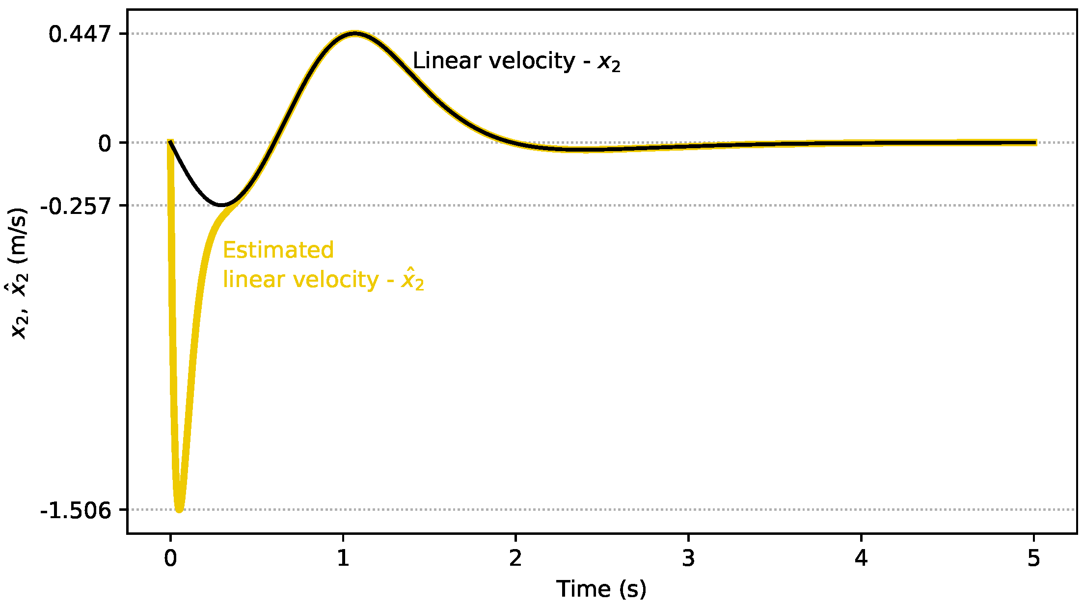
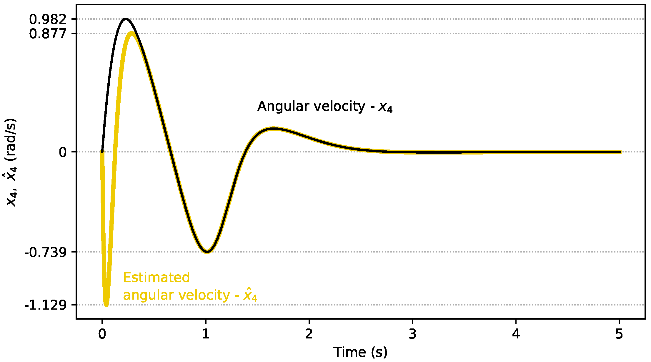
4.1. Linear Observer Results

First, we discuss the behavior of the linear observer outside of the control loop (the structure in Figure 4a). As can be seen in Figure 5 and Figure 6, even the closeness of the initial conditions did not prevent transitional errors. What can be consistently observed among all cases is that the estimation of the linear velocity $x_2$ was simple for both of the observers, and the transitional errors were small. For the estimation of the angular velocity $x_4$, the linear observer needed more time, approximately 1 s. As the time constants of the linearized system error were all less than $0.05$ s, this cannot be considered a satisfactory behavior.

The introduction of the linear observer into the control loop (the structure in Figure 4b) behaved as expected and reduced the control quality. The estimation of the linear velocity was still effective (Figure 7), but as we can see, the system stabilized after 5 s, twice as long as previously. In the case of the angular velocity (Figure 8), we can see that the estimation error, while having relatively moderate transitional errors, converged to zero after more than 3 s. This is the mentioned fragility, as increasing the initial estimation error (different initial condition) caused the system to completely destabilize.

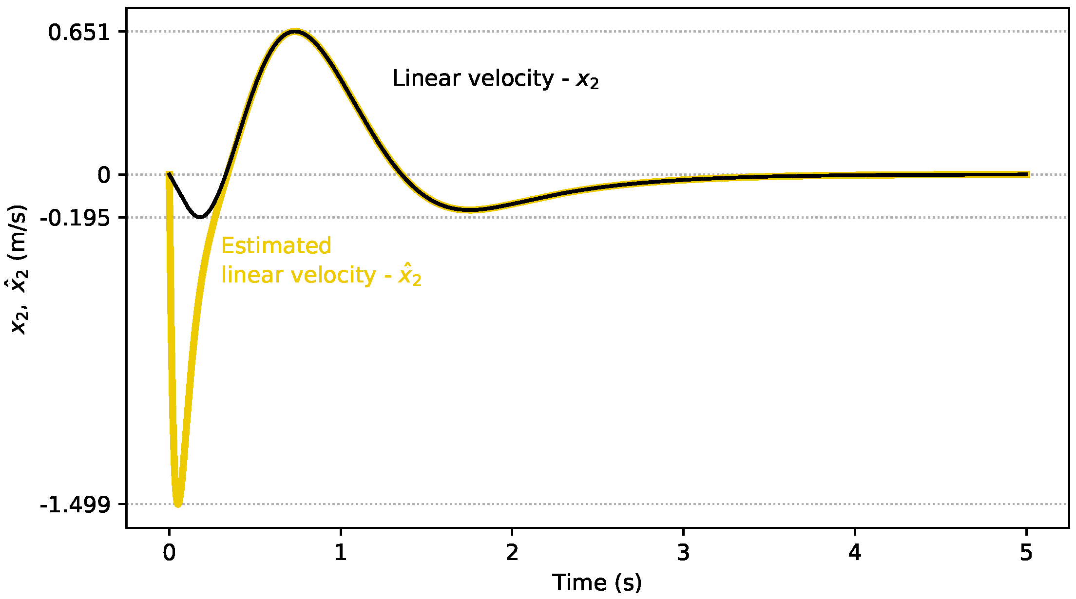
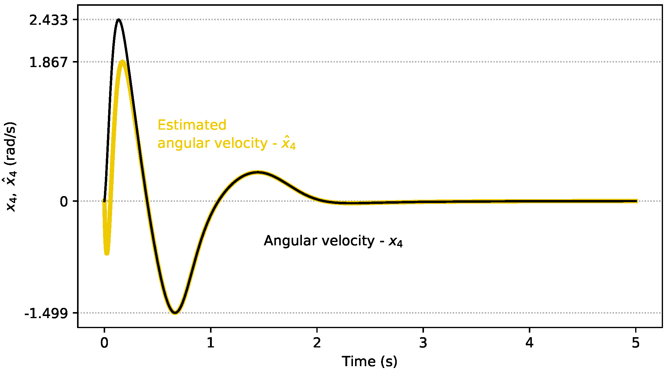
4.2. Nonlinear Observer Results

We follow with the analysis of the nonlinear observer outside of the control loop (the structure in Figure 4c). Because of the stability of the observer, we relaxed the requirements on the initial conditions, and the observer started from 0. The nonlinear observer introduced an effect, known as the “peaking phenomena”, where initially, the estimate had a large transitory error, which can be seen even in the estimates of the linear velocity (Figure 9). This transitional error however vanished after approximately 0.25 s, which was consistent with the time constants of the linear part of the error dynamics −0.05 s. Therefore, the error vanished after 5 time constants. A similar behavior was observed for the angular velocity (Figure 10). In both cases, the transitional error was brief and in the opposite direction to the growth of the state variable.

The introduction of the nonlinear observer into the control loop (the structure in Figure 4d) gave surprising results. First of all, the state estimation of both the linear and angular velocities (Figure 11 and Figure 12) did not differ much from the case of the observer working independently. Moreover, the control quality was not adversely affected by the peaks in the estimation error. Quite the opposite, as the volatility increased at the beginning, this helped obtain the quicker stabilization of the angular velocity.

5. Discussion and Conclusions

In this paper, two methods for the observer design of a highly nonlinear system with a variable moment of inertia were presented. The modeling of this system was presented, along with the methods for the parameter derivation. The observability of the system with respect to the output (17) was verified, and two observers were designed. The first one was the classical linear full-rank observer for the linearized system. The second one was a new idea for a semiglobally stable observer, which in some aspects was similar to the one presented in [51]. For such an observer, the outline of stability proof was presented, based on the circle criterion. The effectiveness of both observers was illustrated with simulations.

The proposed observer structure addressed an interesting problem. When designing state observers for linear systems, the error dynamics is also linear, which simplifies the analysis. In nonlinear systems, this is not so easy. The optimal situation is the so-called output injection, where using the output measurements in the observer instead of the respective state estimates, we can cancel out the nonlinear terms in the error equation. Those systems are, however, rare, and the transformation to them is highly nontrivial. If the nonlinearities are bounded (for example, by the Lipschitz constant), then a Lyapunov function for the error equation can be designed and appropriate bounds used. High-gain observers mix this approach with the transformation in a way analogous to linearizing the feedback. They however have a tendency toward even larger transitory peaks. Sliding-mode observers require the careful design of the sliding surface, which for a four-dimensional system, can be troublesome. That is why the proposed approach stands out. We performed partial output injection and treated the remaining part as a Lurie system that could be handled by a circle criterion to ensure the semiglobal stability. This approach is attractive, but highly unique. However, as was presented, this works both outside and inside the control loop.

The limitations of this approach come from the specificity, as only some systems have this property. Moreover, issues can arise similar to the case of the output injection observers, when the identification is bad and the canceling is only partial.

Further work will include testing this observer with some global control and comparisons with different types of observers.

References

1. Ahmad, B.; Hussain, I. Design and hardware implementation of ball & beam setup. In Proceedings of the 2017 Fifth International Conference on Aerospace Science & Engineering (ICASE), Islamabad, Pakistan, 14–16 November 2017; pp. 1–6. [Google Scholar] [CrossRef]
2. Takacs, G.; Mikulas, E.; Vargova, A.; Konkoly, T.; Sima, P.; Vadovic, L.; Biro, M.; Michal, M.; Simovec, M.; Gulan, M. BOBShield: An open-source miniature ‘ball-and-beam’ device for control engineering education. In Proceedings of the 2021 IEEE Global Engineering Education Conference (EDUCON), Vienna, Austria, 21–23 April 2021; Volume 2021, pp. 1155–1161. [Google Scholar] [CrossRef]
3. Šitum, Z.; Trslić, P. Ball and beam balancing mechanism actuated with pneumatic artificial muscles. J. Mech. Robot. 2018, 10, 055001. [Google Scholar] [CrossRef]
4. Mazenc, F.; Astolfi, A.; Lozano, R. Lyapunov function for the ball-and-beam: Robustness property. In Proceedings of the 38th IEEE Conference on Decision and Control, Phoenix, AZ, USA, 7–10 December 1999; Volume 2, pp. 1208–1213. [Google Scholar] [CrossRef]
5. Sira-Ramirez, H. On the control of the “ball-and-beam” system: A trajectory planning approach. In Proceedings of the 39th IEEE Conference on Decision and Control, Sydney, NSW, Australia, 12–15 December 2000; Volume 4, pp. 4042–4047. [Google Scholar] [CrossRef]
6. Huang, J.; Lin, C.F. Robust nonlinear control of the ball-and-beam system. In Proceedings of the 1995 American Control Conference—ACC’95, Seattle, WA, USA, 21–23 June 1995; Volume 1, pp. 306–310. [Google Scholar] [CrossRef]
7. Teel, A.R. Semi-global stabilization of the ‘ball-and-beam’ using ‘output’ feedback. In Proceedings of the 1993 American Control Conference, San Francisco, CA, USA, 2–4 June 1993; pp. 2577–2581. [Google Scholar]
8. Aguilar-Ibanez, C.; Suarez-Castanon, M.S.; de Jesus Rubio, J. Stabilization of the Ball on the Beam System by Means of the Inverse Lyapunov Approach. Math. Probl. Eng. 2012, 2012, 810597. [Google Scholar] [CrossRef]
9. Lemos, J.; Silva, R.; Marques, J. Adaptive control of the ball-and-beam plant in the presence of sensor measure outliers. In Proceedings of the 2002 American Control Conference, Anchorage, AK, USA, 8–10 May 2002; Volume 6, pp. 4612–4613. [Google Scholar] [CrossRef]
10. Marton, L.; Lantos, B. Stable Adaptive Ball and Beam Control. In Proceedings of the 2006 International Conference on Mechatronics and Automation, Luoyang, China, 25–28 June 2006; pp. 507–512. [Google Scholar] [CrossRef]
11. Turker, T.; Gorgun, H.; Zergeroglu, E.; Cansever, G. Exact Model Knowledge and Direct Adaptive Controllers on Ball and Beam. In Proceedings of the 2007 4th IEEE International Conference on Mechatronics, ICM 2007, Cairo, Egypt, 29–31 December 2007; pp. 1–6. [Google Scholar] [CrossRef]
12. Koo, M.S.; Choi, H.L.; Lim, J.T. Adaptive Nonlinear Control of A Ball And Beam System Using The Centrifugal Force Term. Int. J. Innov. Comput. Inf. Control 2012, 8, 5999–6009. [Google Scholar]
13. Naredo, E.; Castillo, O. ACO-Tuning of a Fuzzy Controller for the Ball and Beam Problem. In Advances in Soft Computing; Lecture Notes in Computer, Science; Batyrshin, I., Sidorov, G., Eds.; Springer: Berlin/Heidelberg, Germany, 2011; Volume 7095, pp. 58–69. [Google Scholar]
14. Xi, Z.; Hesketh, T. Ball and Beam System—Nonlinear MPC Using Hammerstein Model. In Proceedings of the 2nd IEEE Conference on Industrial Electronics and Applications (ICIEA 2007), Harbin, China, 23–25 May 2007; pp. 2294–2298. [Google Scholar] [CrossRef]
15. Uran, S.; Jezernik, K. Control of a ball-and-beam like mechanism. In Proceedings of the 7th International Workshop on Advanced Motion Control, Maribor, Slovenia, 3–5 July 2002; pp. 376–380. [Google Scholar] [CrossRef]
16. Guo, Y.; Hill, D.; Jiang, Z.P. Global nonlinear control of the ball-and-beam system. In Proceedings of the 7th International Workshop on Advanced Motion Control, Maribor, Slovenia, 3–5 July 1996; Volume 3, pp. 2818–2823. [Google Scholar] [CrossRef]
17. Andreev, F.; Auckly, D.; Kapitanski, L.; Kelkar, A.; White, W. Matching control laws for a ball-and-beam system. In Proceedings of the 7th IFAC Workshop on Lagrangian and Hamiltonian Methods for Nonlinear Control, Berlin, Germany, 11–13 October 2000. [Google Scholar]
18. Hauser, J.; Sastry, S.; Kokotovic, P. Nonlinear Control Via Approximate Input Output Linearization—The Ball and Beam Example. IEEE Trans. Autom. Control 1992, 37, 392–398. [Google Scholar] [CrossRef]
19. Ortega, R.; Spong, M.W. Stabilization of Underactuated Mechanical Systems via Interconnection and Damping Assignment. IFAC Proc. Vol. 2000, 33, 69–74. [Google Scholar] [CrossRef]
20. Krishna, B.; Gangopadhyay, S.; George, J. Design and Simulation of Gain Scheduling PID Controller for Ball and Beam System. Proceedings of International Conference on Systems, Signal Processing &Manufacturing Engineering, Dubai, United Arab Emirates, 26–27 December 2012. [Google Scholar]
21. Banu Sundareswari, M.; Then Mozhi, G.; Dhanalakshmi, K. Intelligent Tuning of PID Controller to Balance the Shape Memory Wire Actuated Ball and Beam System. Phys. Mesomech. 2020, 23, 621–630. [Google Scholar] [CrossRef]
22. Chang, Y.H.; Chan, W.S.; Chang, C.W. T-S Fuzzy Model-Based Adaptive Dynamic Surface Control for Ball and Beam System. Ind. Electron. IEEE Trans. 2013, 60, 2251–2263. [Google Scholar] [CrossRef]
23. Asadi, H.; Mohammadi, A.; Oladazimi, M. Stabilization ball and beam by fuzzy logic control strategy. In Proceedings of the Fourth International Conference on Machine Vision (ICMV 2011): Machine Vision, Image Processing, and Pattern Analysis, Singapore, 9–10 December 2011; Zeng, Z., Li, Y., Eds.; International Society for Optics and Photonic: Singapore, 2012; Volume 8349, pp. 711–717. [Google Scholar]
24. Minh, V.; Mart, T.; Moezzi, R.; Oliver, M.; Martin, J.; Ahti, P.; Leo, T.; Mart, J. Performances of PID and Different Fuzzy Methods for Controlling a Ball on Beam. Open Eng. 2016, 6, 145–151. [Google Scholar] [CrossRef] [Green Version]
25. Aziz, N.N.A.; Yusoff, M.I.; Solihin, M.I.; Akmeliawati, R. Two degrees of freedom control of a ball-and-beam system. IOP Conf. Ser. Mater. Sci. Eng. 2013, 53, 012070. [Google Scholar] [CrossRef]
26. Jo, N.; Seo, J. A state observer for nonlinear systems and its application to ball and beam system. Autom. Control. IEEE Trans. 2000, 45, 968–973. [Google Scholar] [CrossRef]
27. Jo, N.; Jin, J.; Joo, S.; Seo, J. Generalized Luenberger-like observer for nonlinear systems. In Proceedings of the 1997 American Control Conference Albuquerque Convention Center, Albuquerque, NM, USA, 6 June 1997; Volume 3, p. 2180. [Google Scholar] [CrossRef]
28. Grabowski, P. Stability of Lurie Systems; Wydawnictwa AGH: Kraków, Poland, 1999. [Google Scholar]
29. Zhou, T.; Zuo, Z.; Wang, Y.; Li, H. Synchronization of Lurie Systems under Limited Network Transmission Capacity with Quantization and One-Step Packet Dropout: An Active Method. IEEE Trans. Syst. Man Cybern. Syst. 2021, 51, 4920–4928. [Google Scholar] [CrossRef]
30. Gruyitch, L.; Bučevac, Z.; Jovanović, R.; Ribar, Z. Structurally variable control of Lurie systems. Int. J. Control 2020, 93, 2960–2972. [Google Scholar] [CrossRef]
31. Zhou, S.; Gao, Y. Bipartite synchronization of coupled Lurie networks with signed graph and time-varying delay. Eur. J. Control 2021, 58, 388–398. [Google Scholar] [CrossRef]
32. Pinheiro, R.; Colón, D. Analysis and synthesis of single-input-single-output Lurie type systems via H mixed-sensitivity. Trans. Inst. Meas. Control. 2021. [Google Scholar] [CrossRef]
33. Sun, C.X.; Liu, X. A state observer for the computational network model of neural populations. Chaos 2021, 31, 013127. [Google Scholar] [CrossRef] [PubMed]
34. Ganobis, M.; Chudyba, P. Model and Control of Variable Moment of Inertia System. Master’s Thesis, AGH—University of Science and Technology, Kraków, Poland, 2006. [Google Scholar]
35. YI, J.; Yubazaki, N.; Hirota, K. Stabilization Controlof Ball and Beam Systems. In Proceedings of the Joint 9th IFSA World Congress and 20th NAFIPS International Conference, Vancouver, BC, Canada, 25–28 July 2001; Volume 4, pp. 2229–2234. [Google Scholar]
36. Bodson, M. Fun control experiments with Matlab and a joystick. In Proceedings of the 2003 42nd IEEE Conference on Decision and Control, Maui, HI, USA, 9–12 December 2003; Volume 3, pp. 2508–2513. [Google Scholar] [CrossRef] [Green Version]
37. Wellstead, P. Introduction to Physical System Modelling; Mathematics in Science and Engineering Series; Academic Press: Cambridge, MA, USA, 1979. [Google Scholar]
38. Ganobis, M. On a control of variable moment of inertia system “ball on beam”. Autom. Akad.-GÓRniczo-Hut. Im. StanisAwa Staszica Krakowie 2008, 12, 197–209. [Google Scholar]
39. Keshmiri, M.; Jahromi, A.F.; Mohebbi, A.; Amoozgar, M.H.; Xie, W.F. Modeling And Control Of Ball And Beam System Using Model Based And Non-Model Based Control Approaches. Int. J. Smart Sens. Intell. Syst. 2012, 5, 14. [Google Scholar] [CrossRef] [Green Version]
40. Elsogc, L. Rachunek Wariacyjny; PWN: Warszawa, Poland, 1960. [Google Scholar]
41. Nijmejer, H.; van der Schaft, A. Nonlinear Dynamical Control Systems; Springer: Berlin/Heidelberg, Germany, 1991. [Google Scholar]
42. Klamka, J. Controllability of Dynamical Systems; Kluwer Academic Publishers: Dordrecht, The Netherlands, 1991. [Google Scholar]
43. Kaczorek, T. Teoria Układów Regulacji Automatycznej; WNT: Warszawa, Poland, 1977. [Google Scholar]
44. Baranowski, J. State estimation in linear multi-output systems-design example and discussion of optimality. Autom. Górniczo-Hut. Im. Stanisława Staszica W Krakowie 2006, 10, 119–131. [Google Scholar]
45. Mitkowski, W.; Baranowski, J. Observer design for series DC motor–multi output approach. In Proceedings of the Materiały XXX Międzynarodowej konferencji z podstaw elektrotechniki i teorii obwodów IC-SPETO, Ustroń, Poland, 23–26 May 2007; pp. 135–136. [Google Scholar]
46. Matlab® Control System Toolbox™. Available online: https://www.mathworks.com/products/control.html (accessed on 10 September 2021).
47. Python Control System Library. Available online: https://python-control.readthedocs.io/en/0.9.0/ (accessed on 10 September 2021).
48. Kautsky, J.; Nichols, N.K.; Dooren, P.V. Robust pole assignment in linear state feedback. Int. J. Control 1985, 41, 1129–1155. [Google Scholar] [CrossRef]
49. Turowicz, A. Teoria Macierzy; Wydawnictwa AGH: Kraków, Poland, 2005. [Google Scholar]
50. Kudrewicz, J. Frequency Methods in the Theory of Nonlinear Dynamical Systems; WNT: Warszawa, Poland, 1970. [Google Scholar]
51. Arcak, M.; Kokotović, P. Nonlinear observers: A circle criterion design and robustness analysis. Automatica 2001, 37, 1923–1930. [Google Scholar] [CrossRef]
Figure 1. Rotating beam with a solid ball.
Energies 14 05850 g001
Figure 2. It is possible to estimate the moment of inertia J b e a m of the beam of length L p by making a physical pendulum with it, by hanging it on a string with a length of L n . As long as the angle α is small, the period of oscillation can be used to compute J b e a m .
Energies 14 05850 g002
Figure 3. The nonlinearity of the error dynamics treated as a Lurie system is constrained to a piecewise quadratically bounded sector. Because of this quadratic growth, it cannot be globally bounded by a linear term, which is why the observer can be made only semiglobally stable. What should be noted, however, is that the values of the nonlinearity depend on the dynamics on the control system, so as long as they are far from the boundary values (so that stabilization works), they are much smaller. Examples of the values taken by the nonlinear function in a closed-loop experiment are marked in black.
Energies 14 05850 g003
Figure 4. The presentation of the control structures used in the testing of the observers (linear and nonlinear), considered in two scenarios. The first one is to use the observer independently of the system ((a) and (c), respectively). In such cases, the system is con-trolled by a state feedback, from the actual system state, and the observer estimates the missing state variables. The second test is based on the observer operating as a part of the control system ((b) and (d), respectively). In such a case, the state feedback is con-structed with the system outputs, and the missing state variables are taken from the observer. Note: The white circle denotes the simple summation element; the black circle, however, can be considered an equivalent to the Simulink™mux block, i.e., joining two signals into a vector of signals fed into the system.
Energies 14 05850 g004
Figure 5. The linear observeroutside of the control loop has no problem estimating the linear velocity x 2 , and its estimate x ^ 2 follows it without a large transitional error.
Energies 14 05850 g005
Figure 6. Even outside of the control loop, the linear observer has difficulties estimating the angular velocity x 4 , and its estimate x ^ 4 , even starting with the same initial conditions, has large transitional errors that take about 1 s to vanish. As the time constants of the linearized system error are all less than 0.05 s, it cannot be considered a satisfactory behavior.
Energies 14 05850 g006
Figure 7. Even as a part of the control loop, the linear observer estimates the linear velocity x 2 very well. However, the system takes much longer to stabilize compared to the controller using full state information.
Energies 14 05850 g007
Figure 8. The linear observer in a closed-loop has many problems estimating the angular velocity x 4 . The estimated x ^ 4 converges to the true value only after 3 s. Transitional errors do not greatly exceed 20%, but overshoots happen in both directions.
Energies 14 05850 g008
Figure 9. The nonlinear observer outside of the control loop quickly converges to the true value of the linear velocity x 2 . However, x ^ 2 has a large transitional error of the opposite sign to the actual value and a large magnitude (300 % of the max attained value). The error dynamics is however very fast.
Energies 14 05850 g009
Figure 10. The nonlinear observer outside of control loop expresses a similar behavior for the angular velocity x 4 as for the linear one. x ^ 4 converges quickly, but with a large transitional error, in this case smaller, but still at the level of 100% in the opposite direction.
Energies 14 05850 g010
Figure 11. The nonlinear observer in the control loop estimates the linear velocity x 2 as well as it does independently. x ^ 2 has a minimally larger transitional error, which vanishes in a similar amount of time.
Energies 14 05850 g011
Figure 12. The nonlinear observer in the closed-loop for the angular velocity x 4 behaves even better than it does individually (at least for this case). The transitional errors in x ^ 4 are much smaller. Moreover, a surprising positive effect of the estimation errors occurs, as the stabilization is minimally faster.
Energies 14 05850 g012