1. Introduction
Water utilities properly treat water for common usage and in some cases for drinking. The practices of most water utilities in developing countries are to disinfect water with chlorine, due to the low cost and easy production [
1,
2,
3,
4,
5]. Chlorination is the method at which water is disinfected from viruses and bacteria. This process occurs in the Drinking Water Treatment Plant (DWTP) and guarantees safe water until the last consumer node. The problem derived from chlorine decay over time due to WDN conditions which many of them does not count with Chlorine Booster Stations (CBS) a way of redistributing doses of disinfectant. Water utilities to supply the minimum Free Residual Chlorine (FRC) at the end of the WDN, add elevated doses of disinfectant at the exit of the DWTP [
6]. Reducing chlorine demand from water utilities derives less chlorine manufacture and energy consumption, and a better perception from consumers in tap water safety improves the quotes collection for water utilities; furthermore, there will be a reduction in bottled water and thus a lower environmental impact [
7]. This is important because chlorine gas is commonly manufactured by electrolysis which in some of its variances uses at least 3560 kWh/Ton Cl
2 [
8]. Regulations in the United States of America (USA) established the maximum residual disinfectant level as 4.0 mg/L, above this level exist the potential risk of eyes/nose irritation and possible stomach discomfort, also a minimum of 0.2 mg/L which guarantee disinfection of pathogenic bacteria [
9]; while there exists different regulations for each country, the World Health Organization (WHO) recommends a maximum FRC concentration of 0.5 mg/L and minimum of 0.2 mg/L in the WDN to guarantee the disinfection of water on consumer nodes.
Low disinfectant concentration at DWTP can result in a poor distribution of chlorine and/or fast chlorine decay [
10]. This concentration scenario has been responsible for a significant number of waterborne disease outbreaks, associated with microorganisms such as
E. coli, norovirus, giardia, cryptosporidium amongst others [
11,
12]. Chlorine decay can occur due to the loss of physical integrity caused by diverse factors, such as (a) water main breaks/repair sites, (b) uncovered reservoirs or covered storage tanks with structural deficiencies, (c) cross connections when inappropriately installed, (d) inadequately maintained backflow prevention devices and the loss of hydraulic integrity as incapability to maintain desirable water flow, water pressure, and high residence of water in pipes (i.e., water age) [
13,
14].
The loss of physical integrity in pipelines allows the entrance of microorganisms and other elements that increase chlorine decay [
13]. As a result, layers of microorganisms attached to the pipeline walls acting as microbial pathogens reservoirs known as biofilms, representing a health risk [
15]. Even after treatment, the disinfectant in water can interact within algal organic matter in reservoirs and produce by-products [
16]. Organic matter from biofilms interact with disinfectant and produce carcinogenic by-products, a chemical group known as Trihalomethanes (TTHM’s) [
17]. The identification of these by-products was studied 30 years ago as potentially harmful chlorinated organic material, the most common by-products being chloroform and haloforms. However, the risk of drinking these unintentional by-products is hard to compare against non-disinfected water [
18,
19], as in recent years the studies on disinfectant by-products have focused on the most toxic. After the large amount of disinfection by-products discovered, it is necessary to prioritize a new common data format and data to archive, extract and classify known by-products from those that have not been studied [
20,
21,
22,
23]. The consumption of drinking water with high concentrations of TTHM’s is associated with bladder cancer, of which at least 47% predominate in those who drank tap water with doses higher than 50 µg/L of TTHM’s, compared with those with 5 µg/L or less [
24].
Several problems have been studied around using chlorine as a disinfectant only from WDS, such as iron pipe corrosion [
25,
26,
27] or by-product formation [
24,
28]. Some authors propose the use of CBS to solve problems caused by the excess of chlorine, the decay of disinfectant over time and the lack of chlorine in some consumption nodes due to the spatiotemporal water-disinfectant distribution [
29,
30,
31,
32,
33,
34,
35]. Usually, the studies set scheduling patterns by groups of six hours [
32]; thus, the operation of each CBS is described by four separate constant mass injections along 24 h [
32,
36,
37,
38]. Some research on CBS focuses on mathematical models to propose the optimal location and injection dosage in the WDS, and others use Artificial Intelligence (AI) [
39]. Using AI and informatics allows the simulation of several scenarios before construction investment of the CBS, thus saving money and time in project development [
40]. This research focuses on selecting the optimal placement and scheduling of CBS for minimizing the operational and constructive cost of CBS with two bio-inspired optimization methods.
2. Materials and Methods
This paper describes reliable solutions for decision makers, finding the optimal location for CBS and correspondent scheduling applying Genetic Algorithms (GA) and Particle Swarm Optimization (PSO) techniques on Net Example 2 from EPANET, modified by Boccelli et al. (1998) to obtain a statistical result from optimization performance. This would represent an improvement in the water quality for customers due to a better distribution of disinfectant. Chlorine scheduling injection per hour is expected to reduce the total of chlorine mass injection in WDN. The objectives of Fitness Function (FF) are to (a) use the minimal number of CBS, (b) guarantee the minimal FRC in all consumer nodes, and (c) reduce the chlorine mass injection per day.
2.1. Bioinspired Algorithms
Nowadays, the evolution in technologies allows computers to respond with optimal solutions for emerging problems. The optimization problems try to choose the best solutions from a set of possible ones considering the point of view of programmer criteria and satisfying specific conditions and limitations [
41]. Two different optimization models are used in this paper: GA and PSO as metaheuristics techniques most used in hydraulic issues [
42,
43,
44,
45,
46,
47]. Like many water utilities, CBS construction and infrastructure depends on economic restrictions for building or improving WDS; therefore, a few CBS are selected that can be built as an objective of the FF to supply the optimal distribution of Chlorine in all WDN and maintain safe drinking water. Optimization in WDS models has been developed with GA as partitioning WDS, in order to minimize the contamination impact [
48] and scheduling of valves closure during contamination incidents [
49], allowing a major understanding in the program process.
2.1.1. Genetic Algorithms (GA)
John Holland and collaborators developed GA at the Michigan University during 60’s and 70’s decades, representing possible solutions as individuals in binary strings [
50,
51,
52]. Selective breeding begins with an empty population pool filled with random solutions in the range of possible values. GA selects (selection process) two parents from the population pool; these individuals are qualified (evaluation process) to solve the problem by FF. The better elements selected from the pool are copied for breeding. The breeding occurs while crossing them over dividing the individual strings at certain points and switching (crossover process), generating a pool of new individuals which could mutate an element of the individual string (mutation process). These form two children, which are added to the child population. This process is repeated until the child population is filled and in each generation selects the best individual to be reproduced with the FF [
51,
53]. GA represents a feasible model since it explores the problem without needing a complete mathematical model. GA’s has been deeply studied in hydraulic issues [
43,
44,
45,
46] even nowadays, as well as the optimal use of chlorine applying CBS [
54].
2.1.2. Particle Swarm Optimization (PSO)
The PSO belongs to bioinspired techniques of Artificial Intelligence; the optimization process is not modeled after evolution but after swarming and flocking behaviors in animals. PSO maintains a single static population whose members are tweaked in response to new discoveries about the space [
53,
55]. All the particles in the search space are rated, then the highest rated particle is selected; while the maximum iteration number or the error criteria is not attained for each particle, its velocity by Equation (1) and position by Equation (2) would be updated, until one of the conditions was accomplished [
56]. PSO has been used in calibration, in water quality models searching the minimal errors applying diverse decay coefficients suggested by PSO [
57], and in the energy optimization of water pumping systems [
58].
where:
2.2. Problem Formulation and Simulation Conditions
To achieve the objectives, the problem formulation is divided into two parts:
Finding the most important CBS locations for guaranteeing supply safe water in all nodes with at least the minimal FRC of 0.2 mg/L in compliance with regulations.
To determine the schedule pattern dosing to reduce the amount of chlorine per day, for reducing economic and environmental impact.
Both formulations consider safe water distribution with FRC upper 0.2 mg/L and lower than 4 mg/L.
Two optimizing algorithms provided by the Matlab tool extensions are applied. The simulations are run in Matlab version R2017b for 64 bits systems and linked to the Toolkit of EPANET for Matlab [
59]. The extension tools used for GA [
60] and PSO [
61] were run with default settings from Matlab and adapted boundaries to the setting problem of minimum and maximum chlorine concentrations. An FF proposition would be developed for both metaheuristics optimization techniques. The first hours of model simulation water distribution are not completed in the WDN because it takes time until the water arrives from the distribution point until the last node. Due to consumer patterns and incomplete mixing in Water Tanks, only the last 24 h of the complete simulation are considered to analyze FRC for all nodes.
2.3. Fitness Function (FF) Formulation
The first objective of the FF should be locating the CBS. The CBS set in EPANET Matlab Toolkit are assigned as Setpoint Booster Stations. GA and PSO would range in the floating rate of zero or maximum concentration, where zero represents a non-station and the maximum concentration represents a CBS with a fixed dosage. This is made to reduce computational efforts by diminishing solution variables, limiting whether the CBS benefits chlorine distribution in the WDS. It is intended to guarantee as many consumer nodes as possible with the minimal FRC, with the location of the new CBS.
The GA and PSO techniques require an evaluation where each scenario is qualified according to the objective. This grading could be any real number defined by the limits of the function.
The penalty in the Fitness Function for achieving the minimal FRC in all consumer nodes contemplates the sum of lags out Chlorine concentration allowed by regulation, i.e., if concentration (C) in the node (i) at the time (t) is lower than minimal FRC (0.2 mg/L), then is applied in Equation (3).
where: C
(i,t) = concentration in the node (i) at the time (t) within last 24 h of simulation, Nn = number of nodes, t = simulation time step, T = last hour of simulation established, C
min = minimal concentration by regulation presented in this study (0.2 mg/L), DEL
(i,t) = matrix with the difference of concentration out of the regulation in each node on the last 24 h.
Else if
> Cmax
where: C
max = maximal concentration by regulation presented in this paper (4.0 mg/L).
Thus, if Cmin then
Finally, DEL represents the total sum of all values out of range in mg/L. Thus, a higher value in DEL represents the worst scenario in chlorine distribution. Additionally, the number of CBS are counted as (NE), initializing NE = 0 and then for all insteps if at the node i exist setpoint booster then NE = NE + 1, and FF1 is given by Equation (6)
where: FF1 = Fitness Function, NE = Number of CBS estimated for each individual.
Firstly, individuals for each optimization model are classified with parameters DEL and NE, so the best individual is that one that minimizes the number of CBS while guaranteeing the minimal FRC in all nodes. Secondly, once the locations of CBS is established, it is proposed that dosage injection of disinfectant would be reduced through a time pattern injection assignation. It is expected that significant reduction of chlorine consumption during the water treatment when applying hourly patterns in chlorine injection optimizes the distribution of FRC around all the WDS. GA and PSO are applied for obtaining the best hourly dosages. FF scheduling evaluates represented by DEL from the FF1 in Equation (6), supplied by the CBS, then with FF2 from Equation (8) the chlorine supply is assured with the least mass injected.
where TMI = sum of all chlorine mass injected on the WDN and converted to kg/day,
= flow passing thru CBS in the node i at time t.
= disinfectant mass added at disinfection location i at time t. Then:
where FF2 = fitness function that seeks to reduce the chlorine mass injection but still guaranteeing FRC in the consumer nodes, TMI = total mass injected by CBS, it is obtained with the toolkit of EPANET for MATLAB and is properly adapted with flow units. The Same FF1 and FF2 are used for both GA and PSO optimization.
Finally, the FF is an alternative way of a multi-objective optimization problem, where arbitrary multipliers between 0 and 1 are assigned as a percentage relevance for each objective in the multi-objective naive function. Additionally, the code is treated as a minimization problem, considering it is more relevant to comply with the FF1 than FF2.
3. Application of the Methodology
The previous methodology for optimizing the water quality with GA and PSO algorithms, considers distributing minimal required Free Residual Chlorine (FRC) throughout all consumer nodes, by using a CBS dosage hourly pattern. The Net Example 2 from EPANET (Case Study 1) is selected to obtain a statistical reference for taking a decision and in a real WDN from Mexico (Case Study 2) the selected algorithm will be implemented.
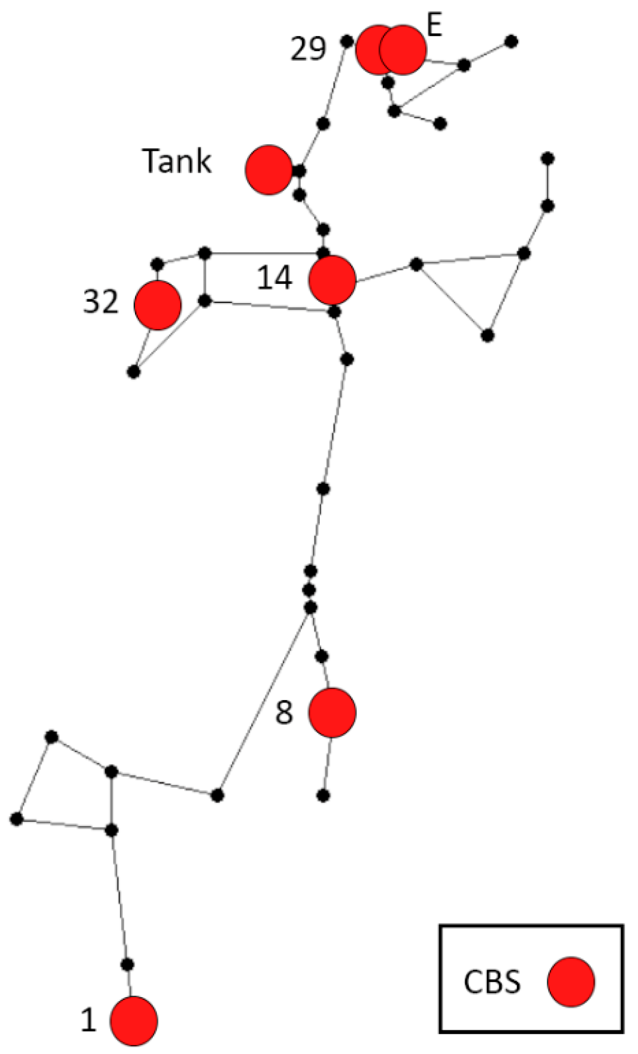
3.1. Case Study 1
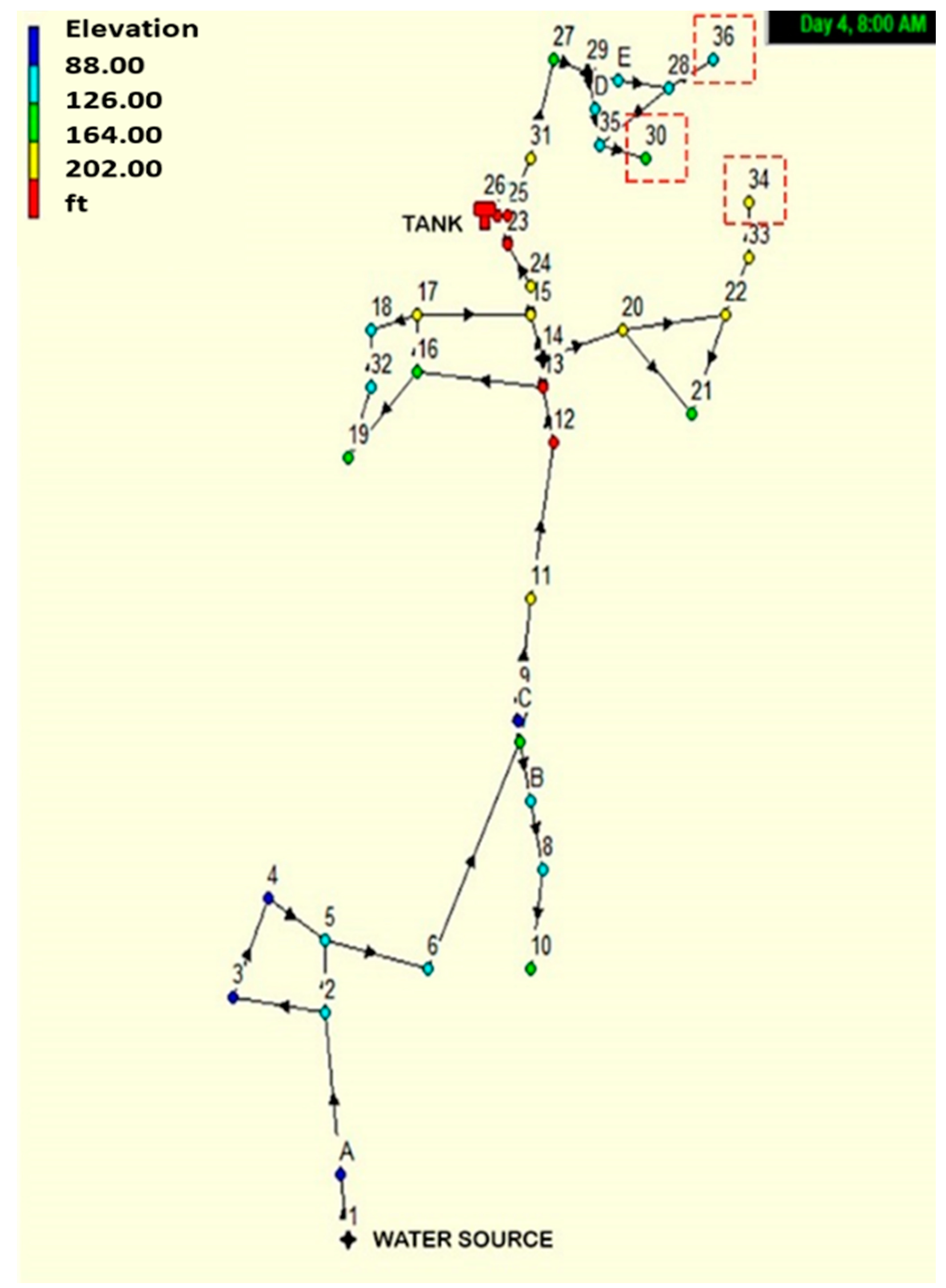
The Case Study 1 applies the methodology presented for the Net Example 2 (
Figure 1) provided by the EPANET toolkit [
62]. This is an existing network in the USA from the Cherry Hill-Brushy Plains and modified by [
32]; while adding nodes (A-F), the WDN includes one water storage tank (node 26), one pumping station (node 1), 41 consumption nodes, and 46 pipes. For comparison with previous works, quality and hydraulic models like consumer and demand multipliers are considered as reported by [
32], there are two pipeline diameters; 8 and 12 inches. The total length of WDN conforms 10.92 kms of pipelines. The bulk chlorine decay constant rate equals 0.5 d
−1 while wall chlorine decay is zero as in previous studies. Additionally, for comparison the values of Minimal Chlorine Concentration of 0.2 mg/L and Maximal Chlorine Concentration of 4 mg/L according to the WDN regulations in the USA are used, the time simulation is 72 h, with 5 min for water quality time step, and 1 h for hydraulic time step [
32].
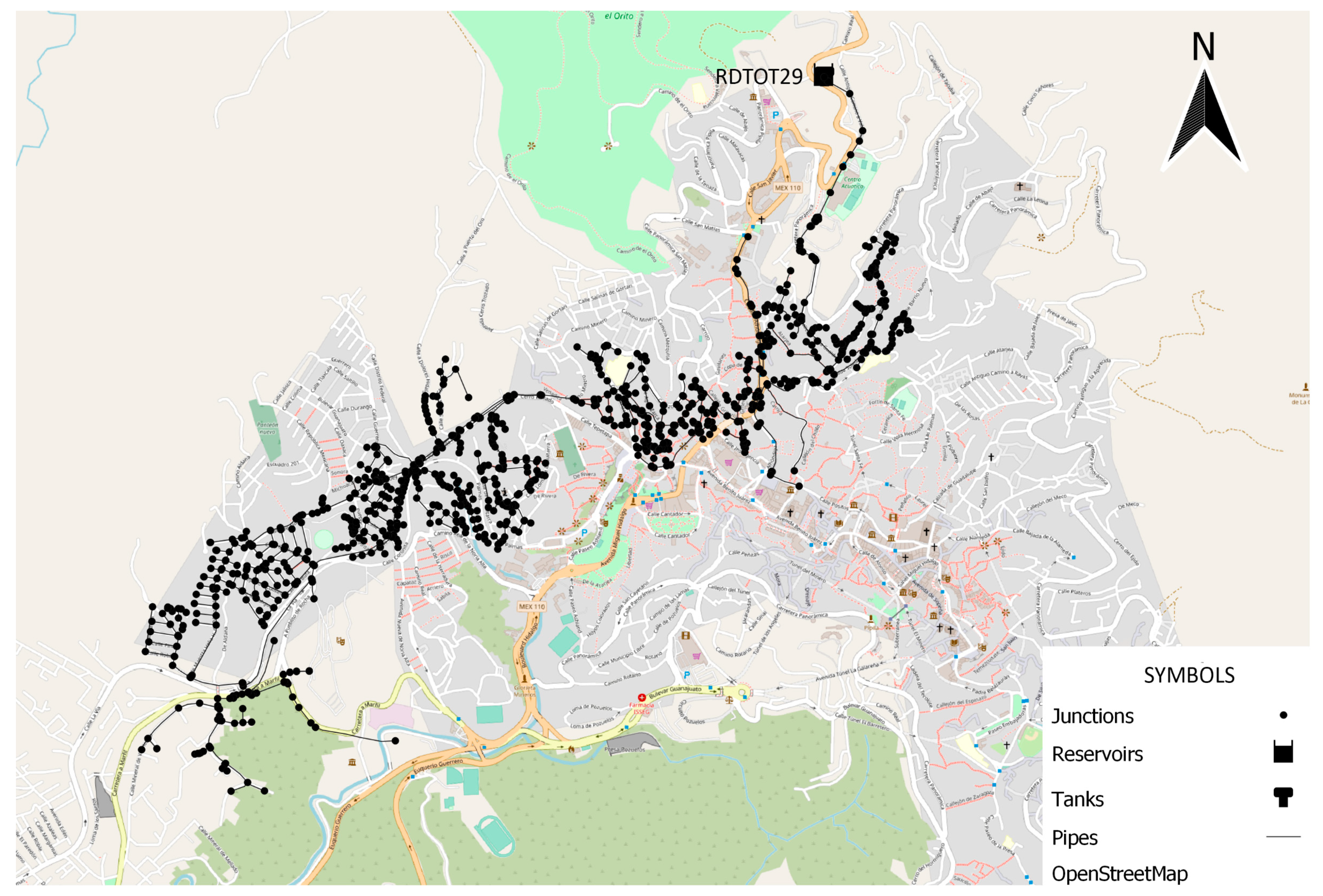
3.2. Case Study 2
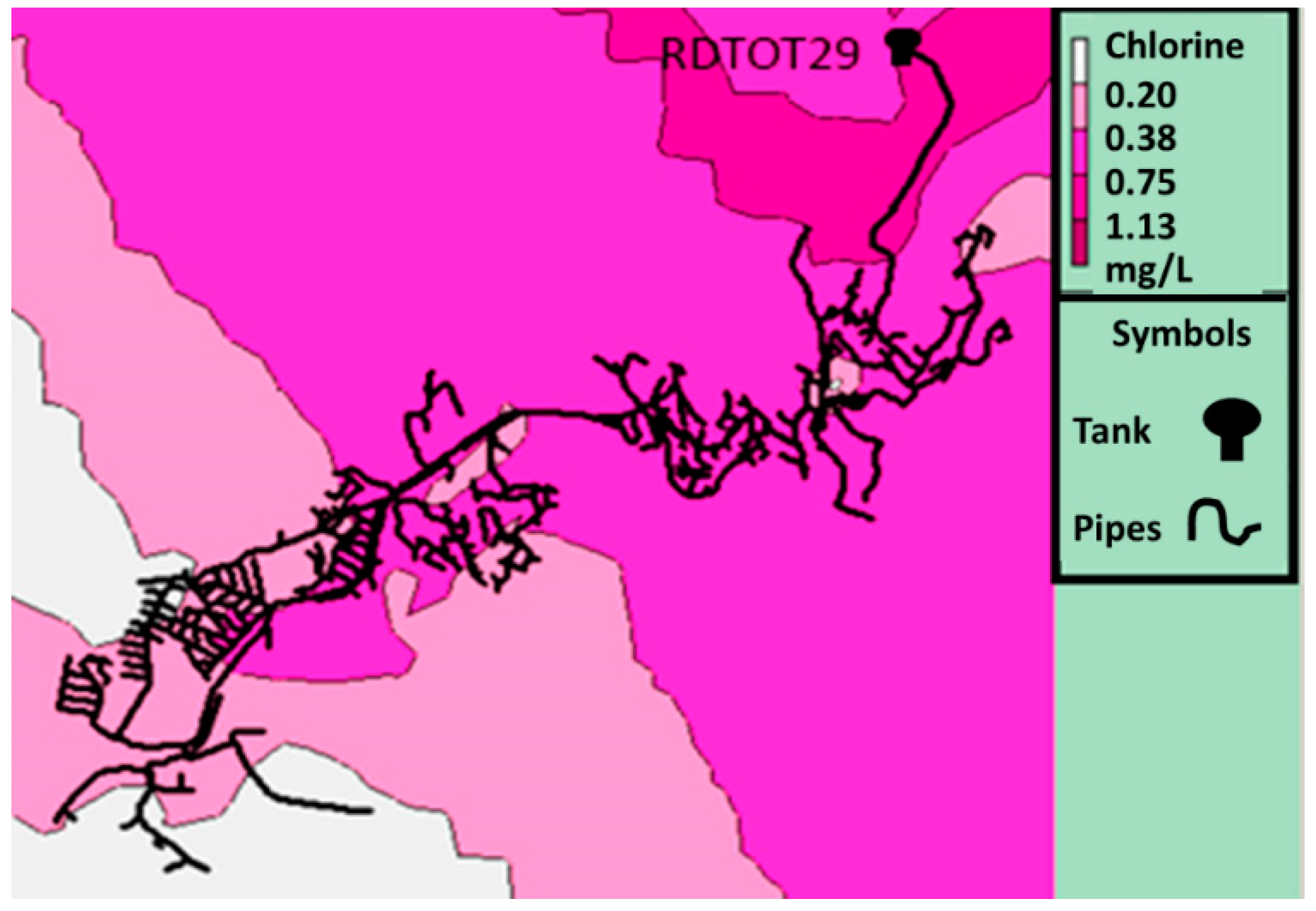
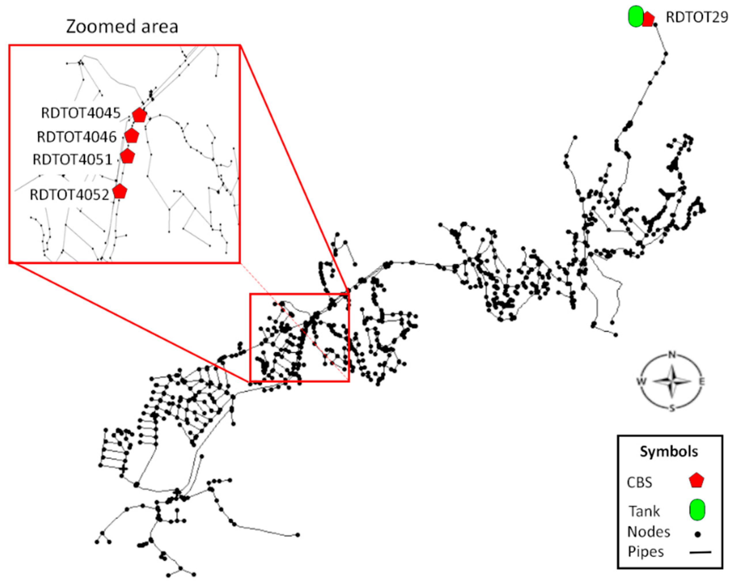
The second WDN is from a location in Guanajuato, Mexico; this network supplies around 34 thousand people, with a mean water consumption of 33.88 L/s, and includes one tank of water distribution with minimum volume of 136 m
3 which is continuously filled (
Figure 2). The distribution work by gravity flowing out from the DWTP (node RDTOT29) in the north-east of the city and ending at the south-west. The local Water Utility Plant provided the model. The pipelines material is mainly PVC and iron, the main pipeline has diameters between 6 to 24 inches, and the rest of pipes are between ¾ and 4 inches, the Hazen–Williams coefficient roughness is from 110 to 140 and the total length pipes is 30.84 kms. The water is supplied from a dam upstream of the city and the DWTP is located near the city, where the disinfection process uses gas chlorine as pre- and post-treatment.
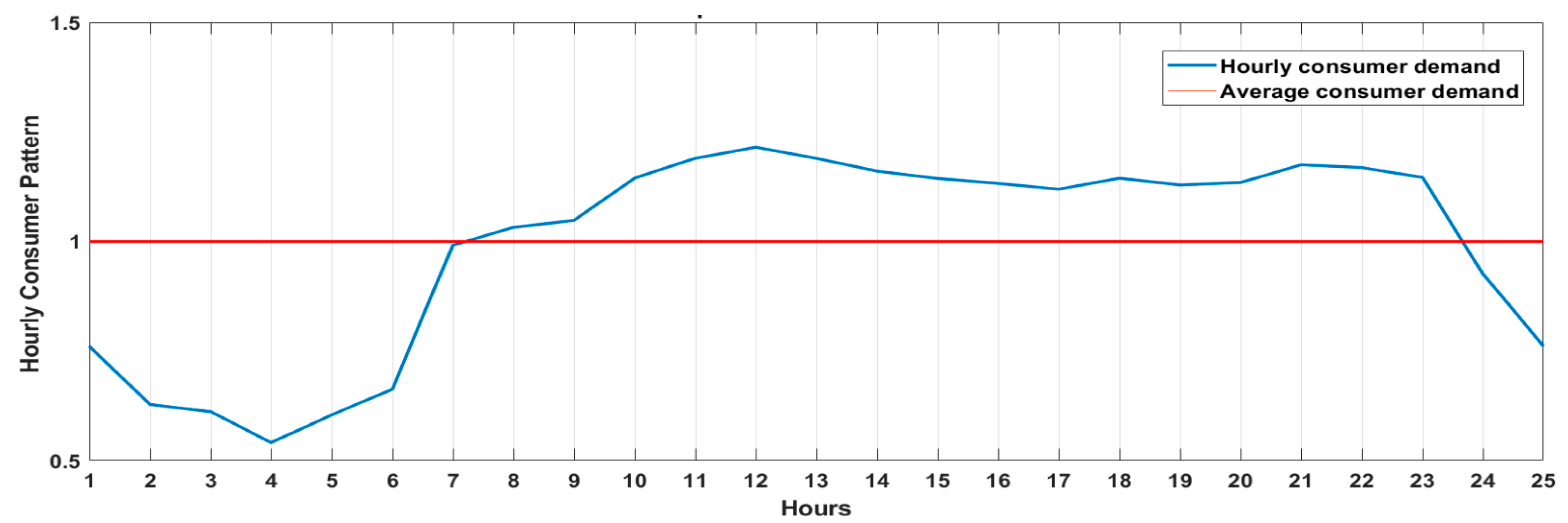
The water demand in the tank (north-east) is identified by the pattern shown in (
Figure 3). It is observed that consumption starts to decrease after 22 h, arriving to the lower demand at 4 in the morning; at 6 am it starts to increase and demand over the mean consumption starts at 7 am until 23 pm with the highest demand at midday.
Originally, it applied an average chlorine concentration of 1.2 mg/L on the node RDTOT29, considered a CBS for modelling purposes. The viability of locating more CBS throughout the network will be studied, which would help distribute the chlorine uniformly according to the local and international organizations recommendations to reduce the total dosage per day.
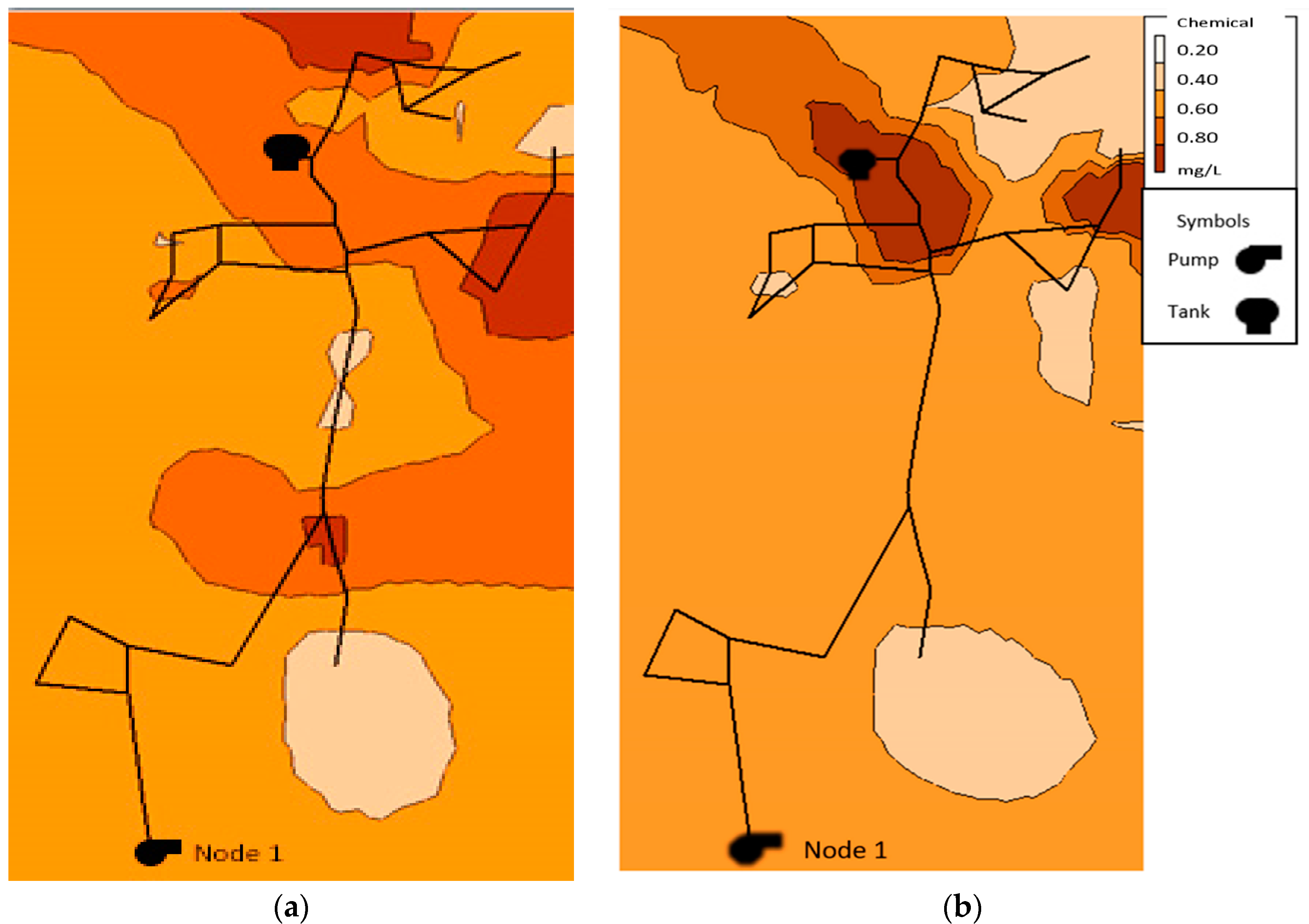
The WDN provided was hydraulically calibrated by a previous simulation to obtain the quality parameters, such as Bulk Decay and Wall Decay coefficients; studies points out the variability in TTHM’S production associated with season changes such as temperature and organic and inorganic materials present from the source [
63,
64]. Thus, the quality model was simulated by 288 h to stabilize the mixing conditions at the tank and obtain steady state conditions for the quality parameters. The calibrated model shows high dose chlorine injection in the DWTP and how chlorine behaves along with the network (
Figure 4). Chlorine might cause organoleptic discomfort to the population near this point because of the smell and the taste; according to a study from Bangladesh, the chlorine taste in tap water was acceptable up to 1.25 mg/L FRC and they were willing to drink because of the safety perception under 2.0 mg/L FRC [
65,
66]. Initial conditions have a mean deviation for FRC in the last 24 h of 0.042 mg/L and a DEL = 340.29 mg/L, using CBS after the node RDTOT29 with a dosage of 14,462 g/d. The Bulk Decay Coefficient is set with 2.04 d
−1 and it has different values of Wall Decay Coefficient with a minimal and maximal of 0.02 and 1.5 m/d, respectively.
4. Results
The evaluations for robustness validation in Case Study 1 were made using PSO and GA with the number of CBS that water utilities can build, considered to be two. Evaluation performances are shown in statistical analysis within 100 simulations. CBS represents the number of boosters stations proposed by the algorithm. CBS simulation reached represents the number of times which that number of CBS was proposed during the 100 simulations. Finally, CBS ID represents the name associated with the node where CBS is proposed.
4.1. Statistical Results from GA Location for Case Study 1
For robustness validation of the optimization process, 100 GA simulations were performed. The results showed that 49% of 100 simulations made by GA guaranteed the minimal FRC in all nodes. The best locations for CBS are presented in
Table 1. It is considered that the most important CBS is located at node 1 with 100% of the simulations proposing a CBS in that node. The second node, proposed by GA to establish a CBS, was the water supply tank in node 26, with 72% of frequency. Other nodes appeared and a result from the usage of 3 or more CBS associated with nodes 14 and 29 and the remaining nodes were dismissed because of their low frequency.
4.2. Statistical Results from PSO location for the Case Study 1
From PSO simulation was obtained 100 simulations to obtain the best locations for CBS (
Table 2). Results have shown higher frequency at the pump station, corresponding to node 1 and the tank, and the others were dismissed due to their low frequency (
Figure 5).
Then, the best and worst individuals are reported by the frequency of CBS ID. It is considered the best individual from the 100 simulations with no penalty in the FF and FRC higher than 0.2 mg/L for all consumer nodes. Thus, the best individual has the FF nearer to the value of one. The individuals with the lower penalty reported CBS location in node 1 (proposed by 100% of simulations) and Water Distribution Tank (proposed by 67% of the simulations). As the main objective was to find the best location for guaranteeing the minimal FRC above all the consumer nodes concentrations, zero or one were selected for representing whether there is chlorine injection in the node or not during the string coding in GA. The optimization algorithm in default settings that worked better on these 100 simulations was PSO.
4.3. Scheduling in CBS Results from GA and PSO
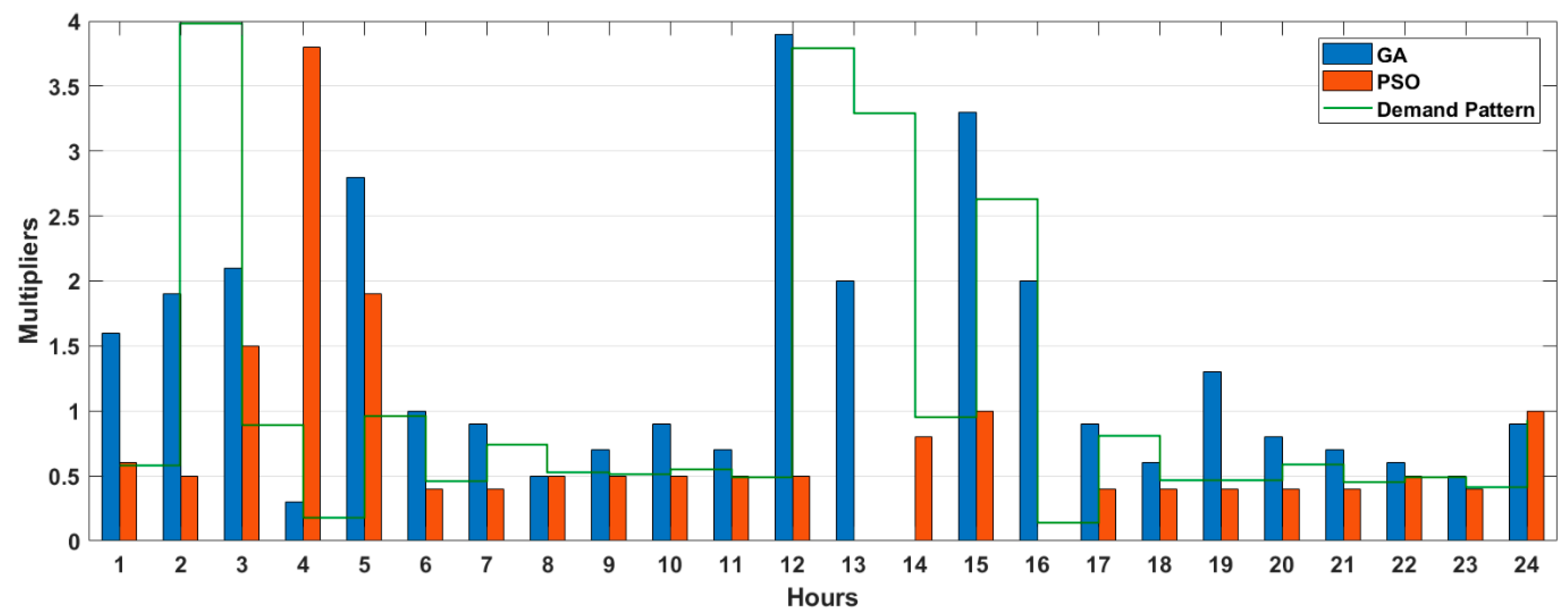
The best location was obtained previously for CBS in Net Example 2. This step aims to determine the schedule pattern dosing to reduce the amount of chlorine per day, thus reducing the economic and environmental impact from water utilities applying the FF2. The optimization consisted in adding hourly multipliers in patterns assigned to the CBS previously selected or presented in the WDN. The patterns are considered by 24 h and if the simulation is larger, then the cycle is repeated. The initial concentration of CBS is considered to be 1 mg/L, so the multiplier would range between regulation values until maintaining the FRC in all consumer nodes and reducing the total dosage of chlorine per day. Thus, those patterns with the lowest dosage per day and the minimal penalty for the tank in
Figure 6. The upper boundary is considered as the maximum chlorine allowed of 4 mg/L and a minimal of 0.2 mg/L, inducing multipliers between those values.
The statistical analysis of scheduling the concentrations in the CBS from the GA shows an average DEL of 0.42 mg/L for 100 simulations and 73% of the simulations reduced the penalty to zero, and only 14% were greater than the average value of the penalty. The best values are obtained in simulation 32 with a zero-penalty value and the lower dosage per day of 1762.75 mg/L. As node 1 works as a pump station, a pattern is assigned (
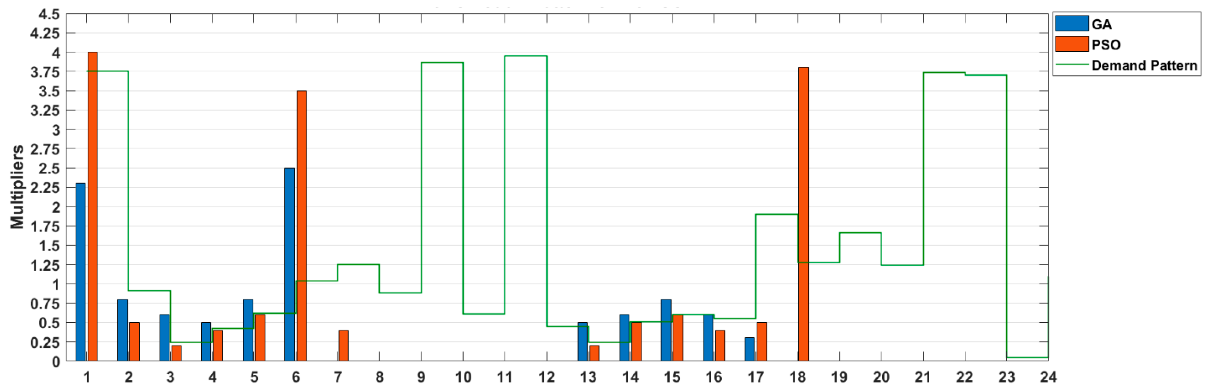
Figure 7), and the injection in WDN from 6 to 12 h and from 17 to 24 h are dismissed because the pump does not supply water in these hours thus chemical neither. The consideration is that at those hours water is distributed from the tank and not from the pump.
Considering the same procedure, the scheduling in CBS results from PSO shows in the statistical analysis of 100 simulations for PSO that 100% of the simulations reduced the penalty to zero. Therefore, the best value focuses on such individuals that dose the minimal mass of chlorine per day, or with zero-penalty value, and the lower dosage of 1279 g/day was founded in the simulation number 27. As the node 1 works as a pump station, an hourly pattern was assigned and there is no chlorine injection to the WDN from 6 to 12 and from 18 to 24 h.
Both cases use two CBS obtained by solutions from GA and PSO, respectively. This condition guaranteed the minimal concentration of FRC in the scenario of the last 24 h.
Figure 8 shows chlorine distribution at hour 72 of simulation, which is considered for dismissing initial water quality conditions and mixing tank effects [
36].
Both results obtained a full coverage with at least 0.2 mg/L. It was observed that PSO proposes lower concentrations of chlorine (total injected chlorine at 1279.00 g/day while GA maintains higher concentrations (total injected chlorine at 1762.75 g/day. Additionally, while GA have the higher concentration of chlorine injection, this has the lower standard deviation of FRC among the network nodes (
Table 3).
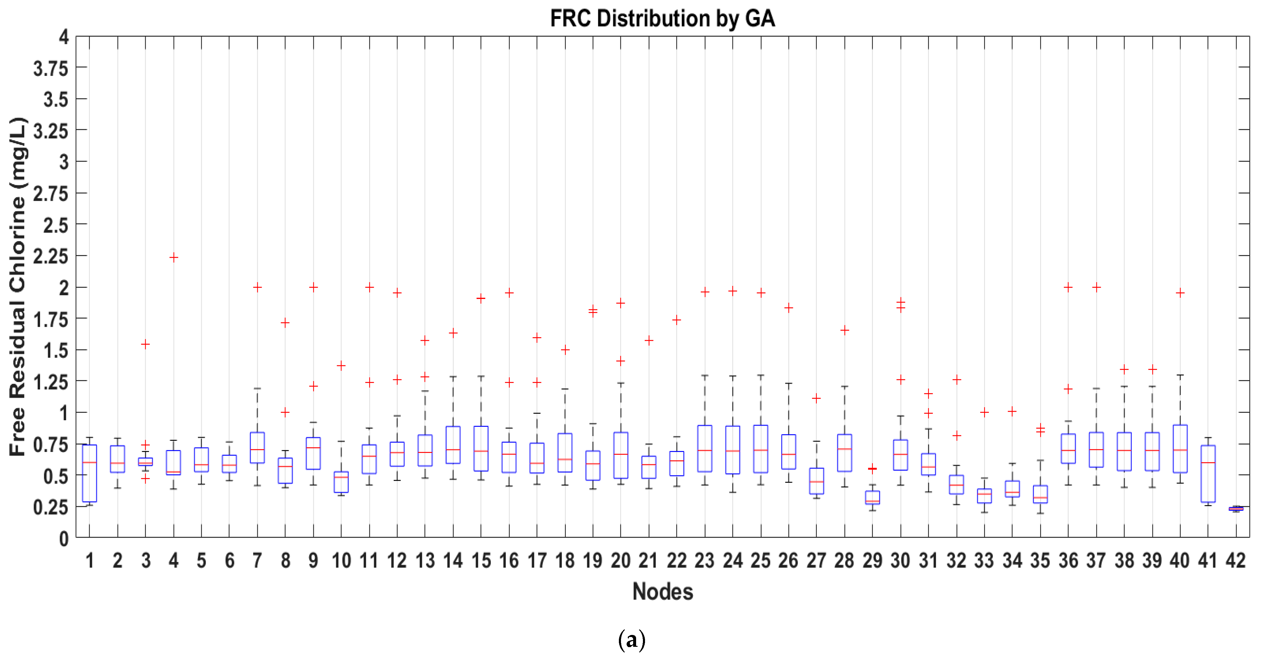
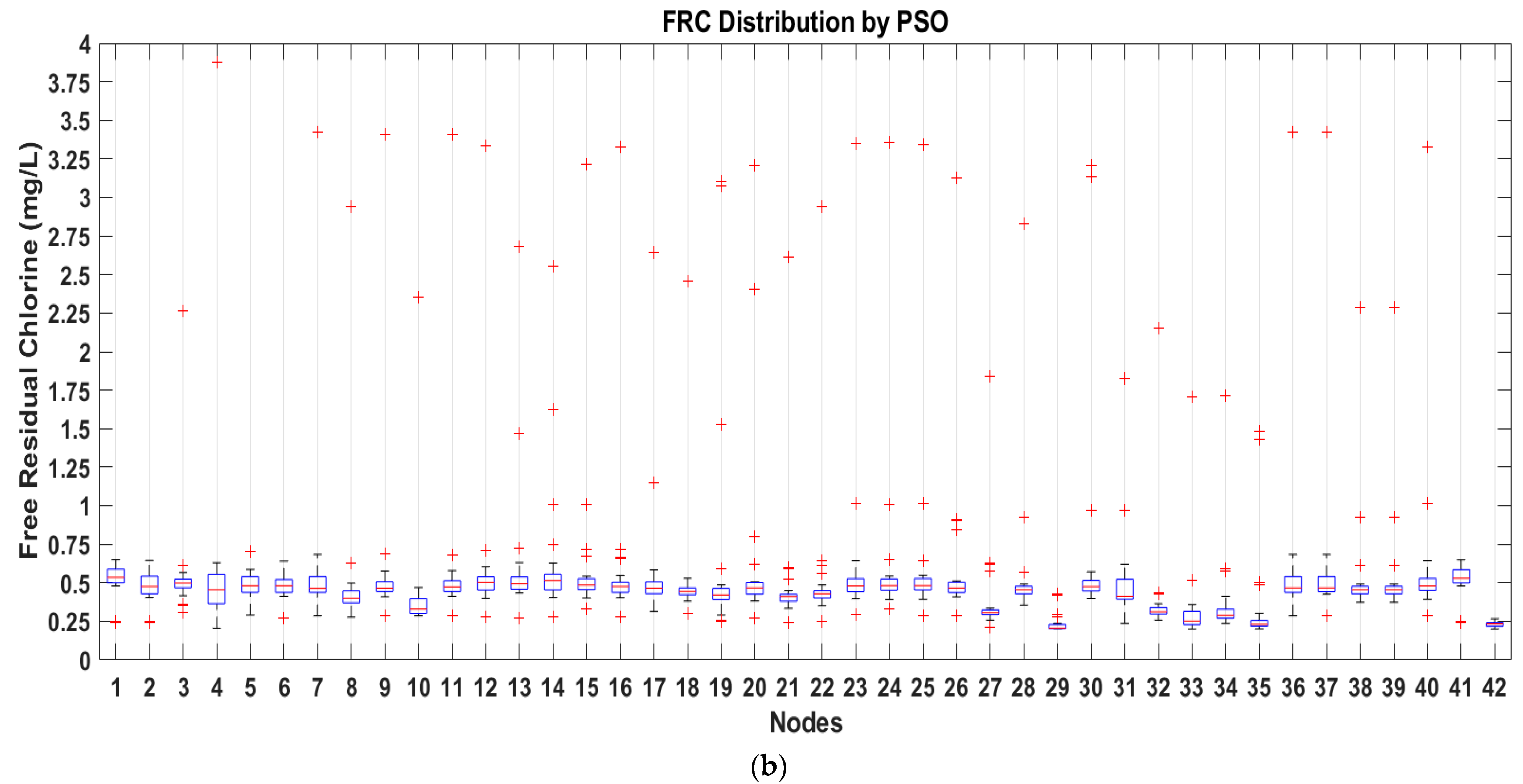
The results of FRC for the last 24 h of simulation for each optimization program showed that GA for most parts of the day remained between the values of 0.25 and 0.8 mg/L (
Figure 9a), while PSO obtained 75% of values equal or lower of 0.6 mg/L (
Figure 9b), plot interpretation can be made with
Figure 10. Therefore, PSO represents a minor concentration of FRC but still guarantees regulated values, which would help reduce corrosion in pipelines and reduce the TTHM’s formations. Both algorithms can solve the problem through trial and error, however the current methodology does not allow parallel processing and as consequence needs more time and computational resources for getting the final solution.
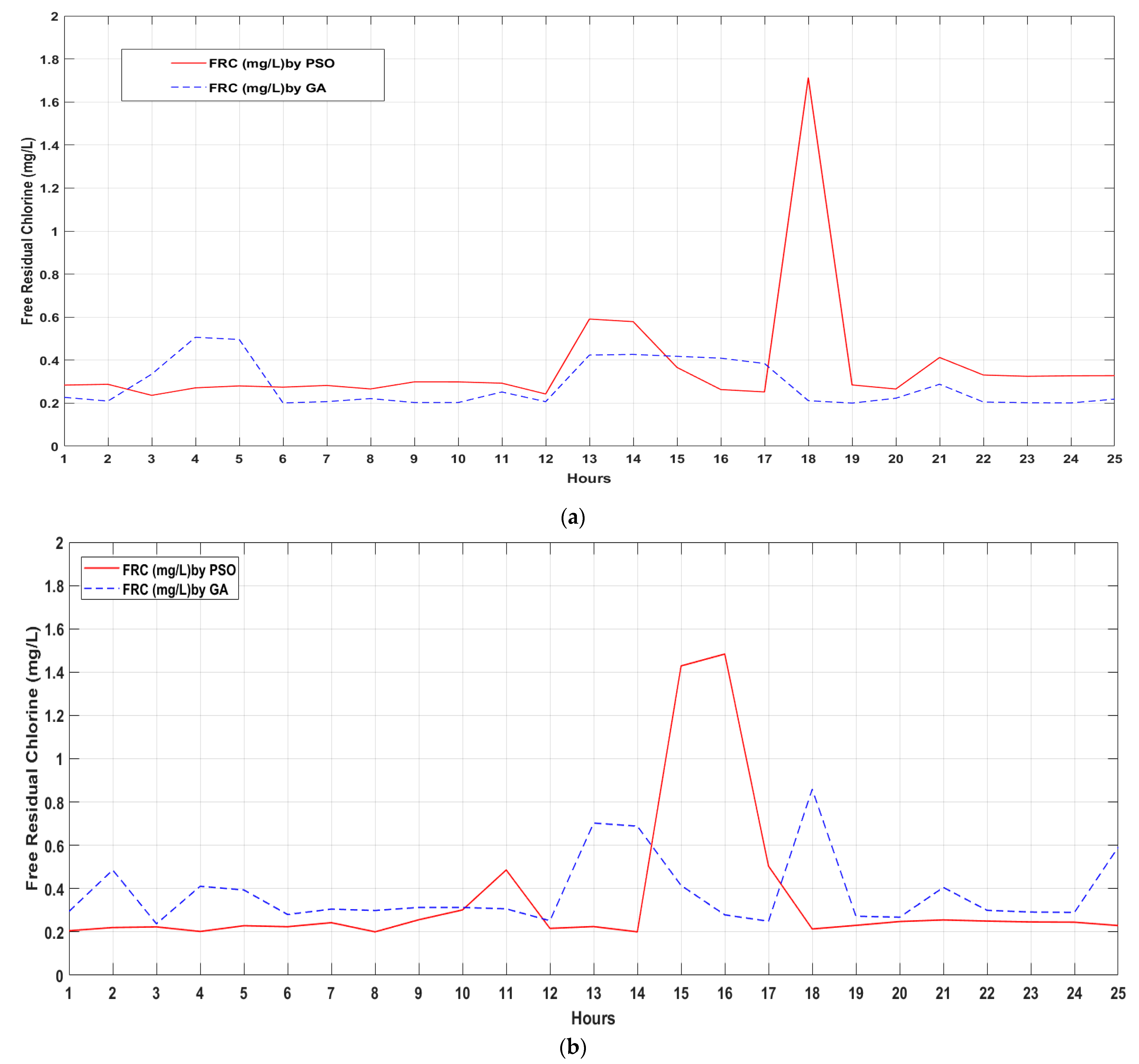
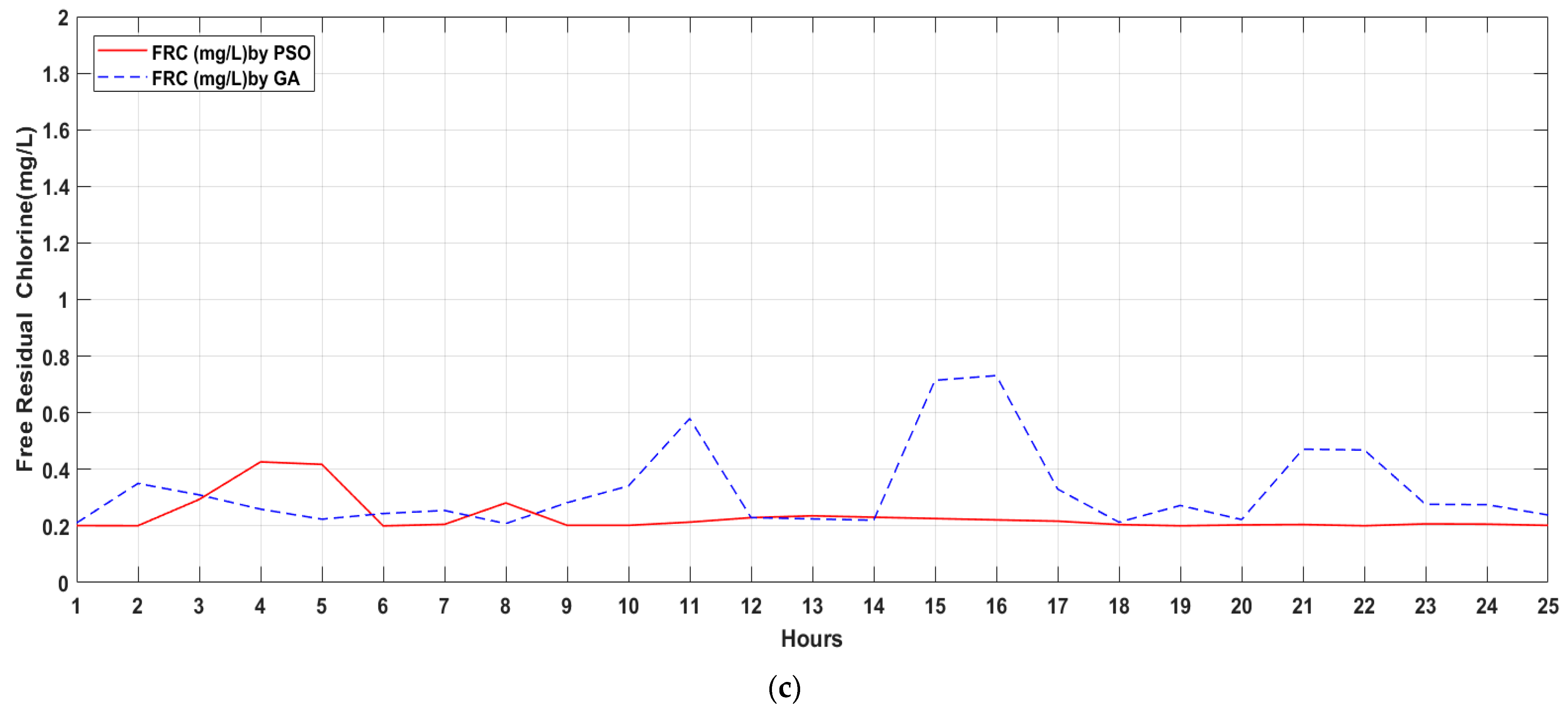
GA results show that even if the concentration injected per day is minimized, nodes; 30, 34 and 36 (
Figure 1 and
Figure 9a), which are farther from the initial distribution point, reach the minimal FRC. In the same way, the FRC concentration in those nodes guarantees the minimal concentration obtained by the method PSO in the last 24 h of simulation (
Figure 9b). FRC analysis from nodes 30, 34 and 36 is presented in
Figure 11a–c, respectively.
4.4. CBS Location and Dosage Results for the Case 1
Multiple analyses were simulated through two different optimization models (GA, PSO). Solutions showed by the optimization models selected the best location for two CBS is near the principal water sources as the pump station in node 1 and node 26 (Water Supply Tank).
Finally, the total mass injected by the CBS obtained with GA and PSO is calculated and compared with those described in the literature review (
Table 4). It can be observed that the total dosage of chlorine injected per day is 1279 g/day for PSO even if the injection patterns are higher at some hours. Additionally, PSO obtained a value of 66 g/day difference with the minimal dosage obtained from Hybrid optimization with solver Harmony Search. As the results of evaluations show that PSO obtained the significant number of feasible solutions in the optimization model for CBS location and scheduling pattern chlorine injection.
4.5. CBS Location Results for the WDN “SF812” in Case Study 2
The WDN “SF812” was evaluated with PSO since previous analysis showed it is more efficient with default settings in the Optimization Matlab Toolkit. It achieved 100% minimal FRC coverage and 71% achieved the goal of established a CBS number decision, which guarantee a reliable solution.
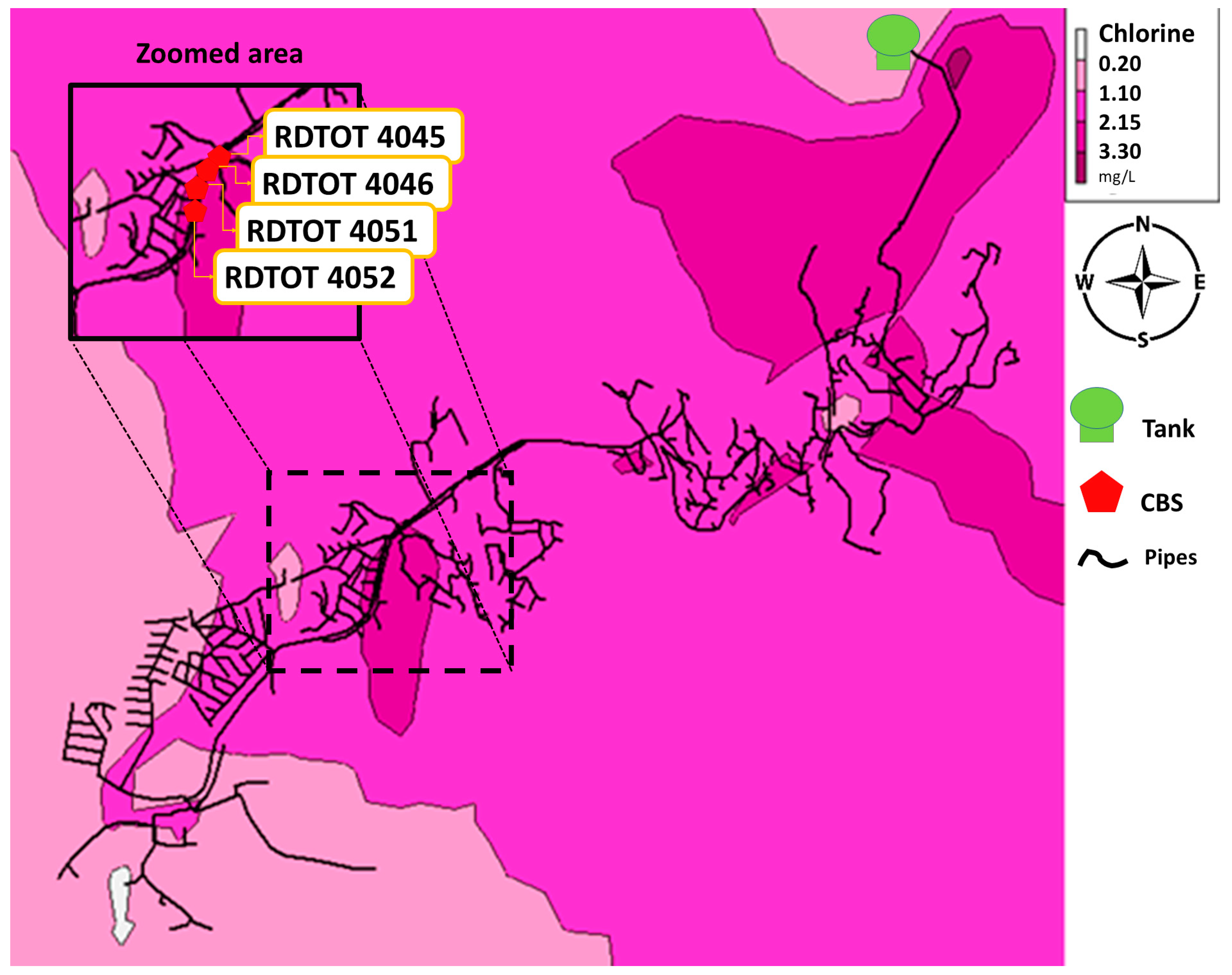
The optimization of chlorine concentration was made considering the CBS location after a time simulation of 232 h. Results proposed 4 CBS in the WDN: RDTOT4045, RDTOT4046, RDTOT4051, RDTOT4052 and a CBS located after the DWTP, in node RDTOT29 (
Figure 12). The minimal distance between the nearer CBS is 9.45 m, meaning the more distant is 64.77 m from each other in this group of CBS. The concentration supplied by each node is the maximum allowed of 4 mg/L in each CBS, which could be due to the severe conditions of chlorine decay in the WDN. The CBS locations are in the southwest of the WDN, which represents more than half of the way until the last node supplied by the tank since the sector after this area has the higher quality problems in the WDN.
Figure 13 shows the chlorine distribution at hour 288 of simulation, with non-scheduled CBS with 4.0 mg/L at each one, a coverage in all consumer nodes with minimal FRC, except (1) the source, which is before the chlorine station, and (2) node RDTOT51 which closes sector with a valve in that point.
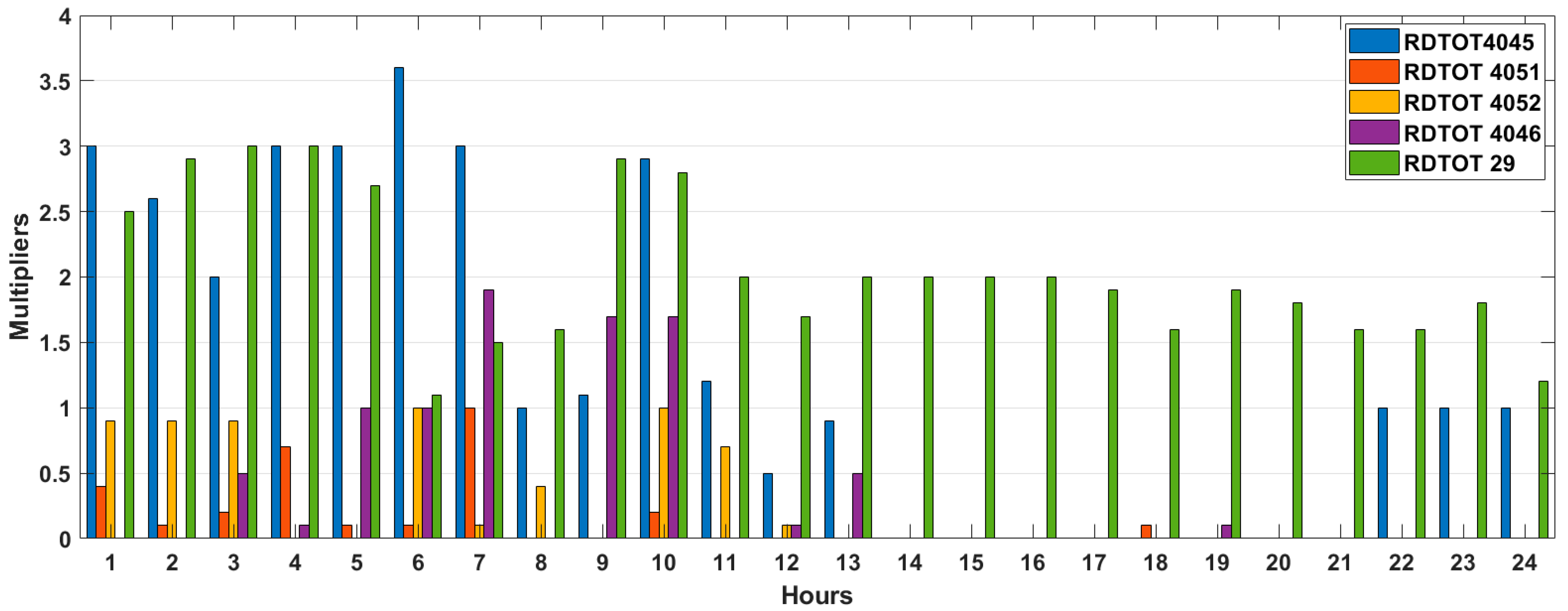
The proposal of scheduling with PSO (
Figure 14) received a penalty DEL = 5.33 mg/L and a total chlorine injection in the net of 21,912.82 g/day. This increment in the chlorine injection is because of the increment in the range of chlorine injection, and the objective of covering all consumer nodes with minimal FRC, the mean standard deviation is 0.042 mg/L, in the last 24 h for all nodes, and non-consumer nodes with base demand of zero were dismissed. As shown in
Figure 14, node RDTOT29 distributes chlorine 24 h per day while auxiliary CBS focuses on distributing chlorine during the night period. This happens because during the night consumers are sleeping, and the water remains in the pipe system, so the water is mainly taken from the pipelines rather than the tank.
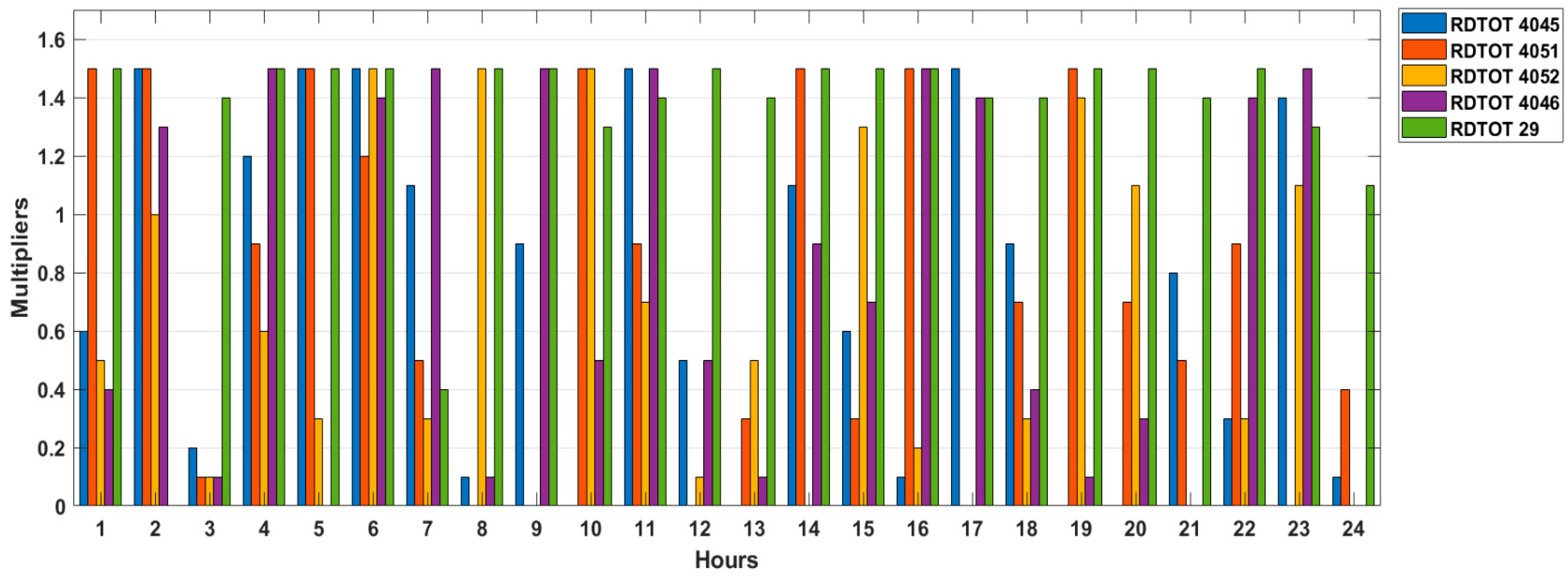
Then, to obey local regulations from Mexico [
67], chlorine limit ranges are proposed between 0.2 and 1.5 mg/L for scheduling simulations in
Figure 15. Thus, multipliers patterns are assigned to hourly distribution to the initial injection of 1 mg/L. Results show a dosage injection of 14.52 kg/day of chlorine mass, and DEL = 57.85 mg/L. In the chlorination pattern, it can be observed that the quantity of chlorine that can be injected most of the time in RDTOT29 was reduced, and auxiliary CBS works at the top amount of chlorine allowed. This is due to severe conditions in the network associated with chlorine decay coefficients.
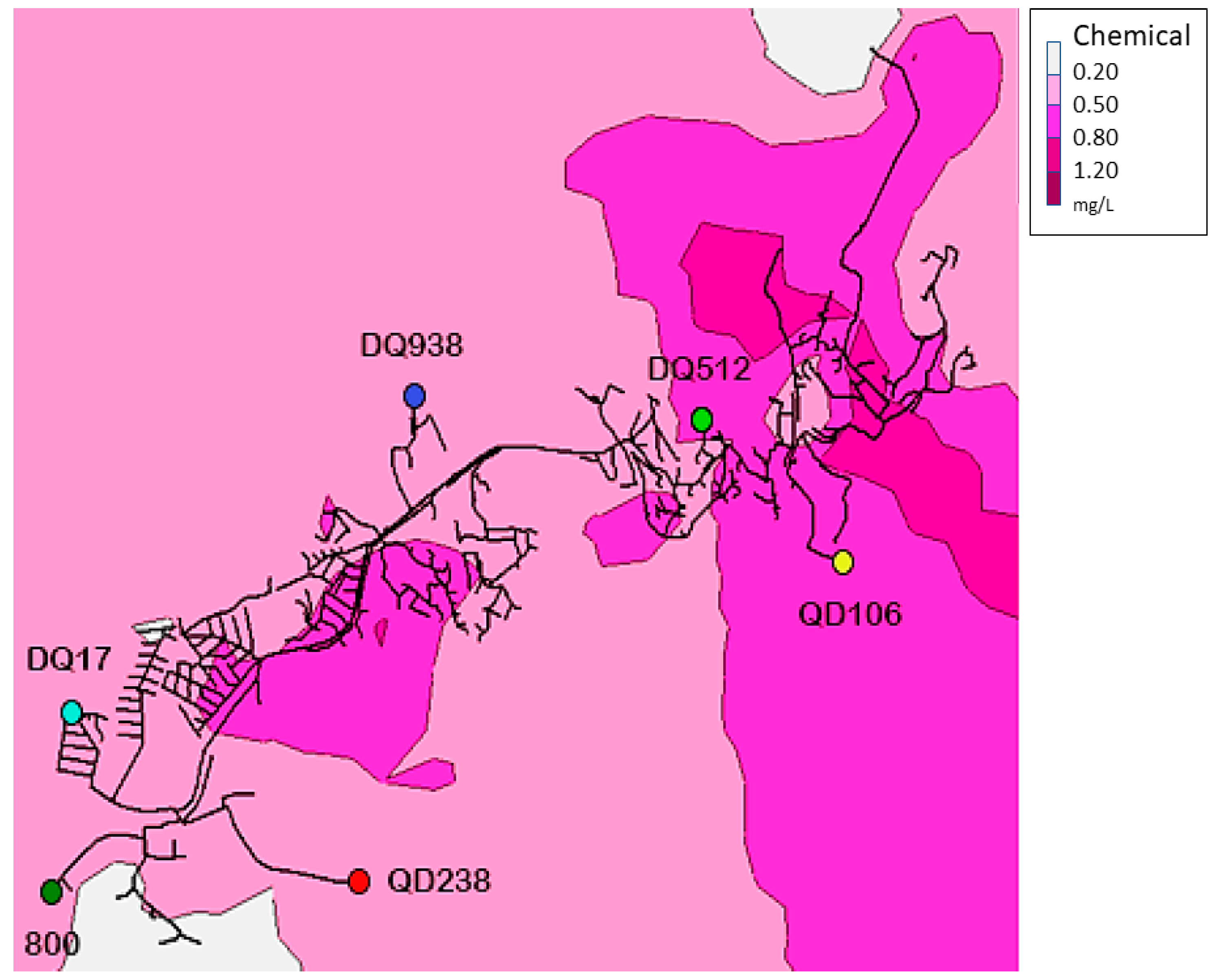
Figure 16 shows the contour plot of time statistical mean FRC applied from the pattern in CBS, as shown in
Figure 15. As the network remains between FRC Mexican regulations, some points at the end (south-east) of the network which do not comply with the minimum values. Thus, critical nodes are presented (
Table 5) and evaluated. These nodes were selected due to their characteristics as elevation, position, and flow velocity from the nearest link.
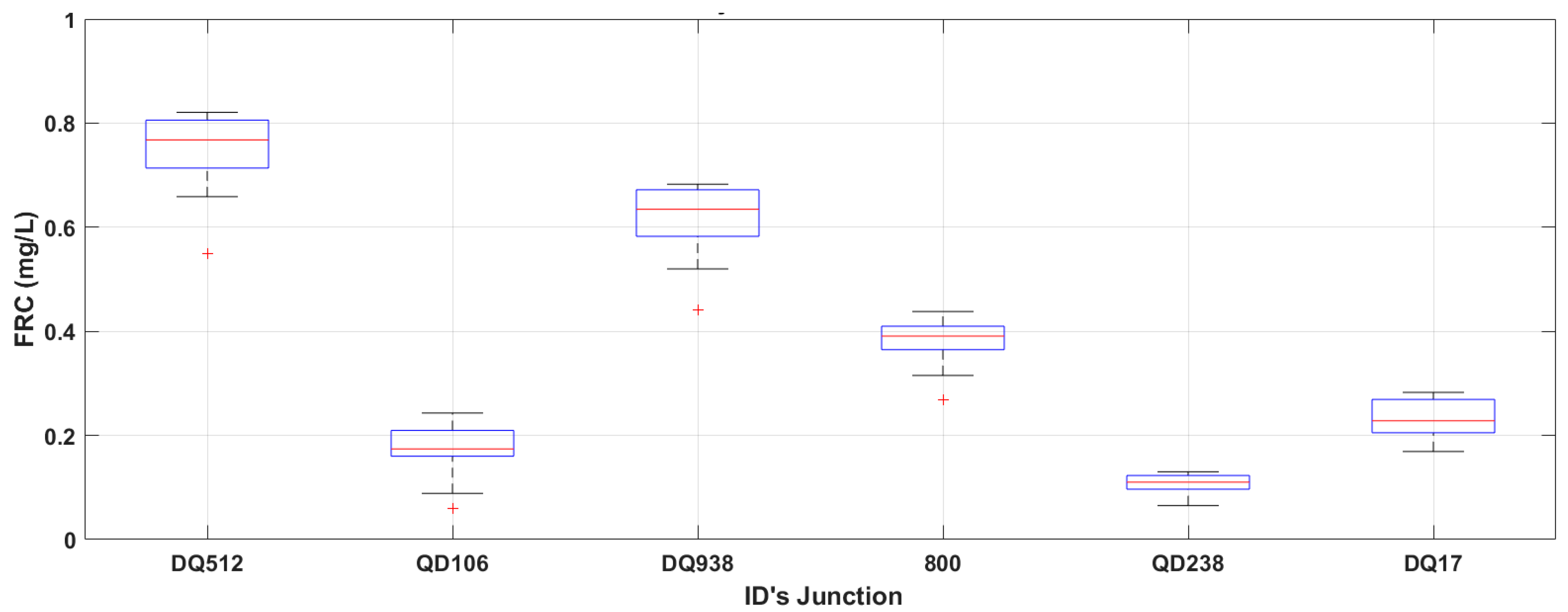
The obtained results from the pattern limit injection between 0.2 and 1.5 did not guarantee the minimum FRC required in the net due to severe conditions of the network as topography and initial water conditions. However, the application represents a significant improvement to the initial conditions of the network, maintaining a mean FRC of 0.71 mg/L, as well from the total simulation time guaranteed the nodes the FRC upper 0.2 mg/L in 95.85%, as we can see in statistical results (
Table 6). From nodes DQ238 and QD106 where box and whiskers plot for critical nodes (
Figure 17) minimal FRC could not be obtained; most problems are related to uneven surfaces and low demand, which translates into long-time water stagnation in pipes and CBS would not be a feasible solution. Implementation of CBS in the WDN improves the water quality with a better chlorine distribution and, as a collateral effect, diminishes the risk of disinfection by-product formation.
5. Discussion and Conclusions
Results of the optimization in case study 1 were compared amongst other literature reviews, thus validating the effectiveness of the fitness function implemented. A reduction of chlorine mass injection was observed. Therefore, the consumption of energy and environmental impact is also reduced as a consequence of a lower consumption and production of chlorine disinfectant. For Case study 2, due to the severe conditions associated with topography, consumer patterns from their floating population, and chlorine decay coefficients, it highlights the need for continuous monitoring points to have total certainty of the model and the need of CBS for better chlorine distribution.
This investigation demonstrated that multi-objective formulation applied in GA and PSO can propose an efficient methodology for CBS locations to guarantee minimal FRC in all nodes (healthy objective) and the minimal number of CBS with the minimal chlorine dosage per day as well (economic and environmental objective). In this case, the trustworthy optimization model was the PSO, which reached coverture in all simulations and the objective of minimal FRC compared with GA, which only 49% of simulated results guaranteeing the minimal FRC in both case studies. Optimizing in two steps seems to be more efficient in the reduction of search space, and variables.
The CBS proposal in Case study 1 guaranteed the minimum FRC for all nodes. It is observed that the use of injection patterns by hour diminish the dosage occurring per day, therefore reducing the health and environmental impact associated with manufacturing and consumption. Chlorine injection patterns show peaks associated with hydraulic consumption patterns and still guaranteeing associated regulations.
The WDN called “Sector 8–12” in Mexico represents a challenge for the local water utility due to the high levels of bulk and wall chlorine decay coefficients. Thus, the algorithm proposes locations for CBS where the disinfectant can be distributed over all consumer nodes with the minimal Free Residual Chlorine. The use of Chlorine Boosters in the network helps to disinfect water over time and chlorine consumption, representing savings for the local water operator and reducing the risk of corrosion in metal pipes, as well as the formation of by-products. On the other hand, reduction of chlorine mass consumption was not achieved. The implementation of time series for chlorine booster stations represents a better solution within both algorithms used in the present work for better chlorine distribution.
Improving water quality on water distribution systems strengthens the confidence of consumers. Thus, the consumption of tap water increases while consumption of bottled water decreases, reducing the environmental impact.
Difficulties presented during the project were mainly caused because the lack of information in Case study 2, future related studies should point at the Internet of Things (IoT) as a tool for improving water distribution systems, and cost benefit analysis considering environmental impact on the use of Chlorine Boosters.
Author Contributions
Conceptualization, J.d.J.M.R., D.H.C. and J.D.P.S.; methodology, B.M.B., G.M.L. and J.D.P.S.; software, D.A.G.C. and J.D.P.S.; validation B.M.B. and J.D.P.S.; formal analysis, J.D.P.S.; investigation, J.D.P.S. and D.A.G.C.; data curation, J.D.P.S.; writing—original draft preparation, J.D.P.S. and B.M.B.; writing—review and editing, B.M.B., J.d.J.M.R. and H.M.R.; visualization, J.D.P.S.; supervision, B.M.B., G.M.L., H.M.R., J.d.J.M.R. and X.D.G.; project administration, X.D.G. and G.M.L.; funding acquisition, X.D.G., H.M.R. and J.d.J.M.R. All authors have read and agreed to the published version of the manuscript.
Funding
CERIS—Civil Engineering Research and Innovation for Sustainability—an FCT-registered research unit operating in the Civil Engineering area. It is hosted by the Department of Civil Engineering, Architecture and Georesources (DECivil) of Instituto Superior Técnico (IST), University of Lisbon (ULisboa).
Institutional Review Board Statement
Not applicable.
Informed Consent Statement
Not applicable.
Data Availability Statement
The data presented in this study are available on request to J.D.P.S.
Acknowledgments
Authors thanks to water system of SIMAPAG for providing their valuable time and information as the modeled case study 2. To CONACYT, Mexican Government for the scholarship of the first author. To Daniel García for taking water samples and calibration of quality model. Additionally, also, to SRE of Mexican Government for the humanitarian flight from Brazil to Mexico during the pandemic season. Thanks to Universidad de Guanajuato, Dirección de Apoyo e Investigación al Posgrado for the economic support for the research stay in Brazil, with grant number DAIP/DGP/300, División de Ingenierías grant number 200501 1720780102 P0701.001 441 254-E06 80-P2893 and Campus Rectoría grant number 200101/P0401.168.201/1120780101/4441/253-E06801-P2857. Also, we would like to thank for financing the payment for publishing the current paper to; CERIS—Civil Engineering Research and Innovation for Sustainability –an FCT-registered research unit operating in the Civil Engineering area. It is hosted by the Department of Civil Engineering, Architecture and Georesources (DECivil) of Instituto Superior Técnico (IST), University of Lisbon (ULisboa).
Conflicts of Interest
The authors declare no conflict of interest. The funders had no role in the design of the study; in the collection, analyses, or interpretation of data; in the writing of the manuscript, or in the decision to publish the results.
References
- Chang, D.; Allen, D.T. Minimizing Chlorine Use: Assessing the Trade-offs Between Cost and Chlorine Reduction in Chemical Manufacturing. J. Ind. Ecol. 1997, 1, 111–134. [Google Scholar] [CrossRef]
- Burch, J.; Thomas, K.E. An Overview of Witter Disinfection in Developing Countries and the Potential for Solar Thermal Water Pasteurization; National Renewable Energy Laboratory: Golden, CO, USA, 1998. [Google Scholar]
- Arnold, B.F.; Colford, J.M. Treating Water with Chlorine at Point-of-Use to Improve Water Quality and Reduce Child Diarrhea in Developing Countries: A Systematic Review and Meta-Analysis. Am. J. Trop. Med. Hyg. 2007, 76, 354–364. [Google Scholar] [CrossRef] [PubMed] [Green Version]
- Fitzmaurice, A.G.; Mahar, M.; Moriarty, L.F.; Bartee, M.; Hirai, M.; Li, W.; Gerber, A.R.; Tappero, J.W.; Bunnell, R.; GHSA Implementation Group. Contributions of the US Centers for Disease Control and Prevention in Implementing the Global Health Security Agenda in 17 Partner Countries. Emerg. Infect. Dis. 2017, 23, S15–S24. [Google Scholar] [CrossRef] [PubMed] [Green Version]
- Reiff, F.M.; Roses, M.; Venczel, L.; Quick, R.; Witt, V.M. Low-Cost Safe Water for the World: A Practical Interim Solution. J. Public Health Policy 1996, 17, 389–408. [Google Scholar] [CrossRef]
- Turgeon, S.; Rodriguez, M.J.; Thériault, M.; Levallois, P. Perception of drinking water in the Quebec City region (Canada): The influence of water quality and consumer location in the distribution system. J. Environ. Manag. 2004, 70, 363–373. [Google Scholar] [CrossRef]
- Delpla, I.; Legay, C.; Proulx, F.; Rodriguez, M.J. Perception of tap water quality: Assessment of the factors modifying the links between satisfaction and water consumption behavior. Sci. Total Environ. 2020, 722, 137786. [Google Scholar] [CrossRef]
- Noval Goméz, L. El Cloro Producción e Industria. Master’s Thesis, Universidad Nacional de Educación a Distancia, Madrid, Spain, 2017. [Google Scholar]
- United States Environmental Protection Agency. National Primary Drinking Water Regulations. Available online: https://www.epa.gov/ground-water-and-drinking-water/national-primary-drinking-water-regulations#Disinfectants (accessed on 9 May 2021).
- Bertelli, C.; Courtois, S.; Rosikiewicz, M.; Piriou, P.; Aeby, S.; Robert, S.; Loret, J.-F.; Greub, G. Reduced Chlorine in Drinking Water Distribution Systems Impacts Bacterial Biodiversity in Biofilms. Front. Microbiol. 2018, 9, 2520. [Google Scholar] [CrossRef] [Green Version]
- Besner, M.-C.; Prévost, M.; Regli, S. Assessing the public health risk of microbial intrusion events in distribution systems: Conceptual model, available data, and challenges. Water Res. 2010, 45, 961–979. [Google Scholar] [CrossRef]
- Craun, G.F. Waterborne Diseases in the US; CRC Press: Boca Raton, FL, USA, 2018; ISBN 1-351-08611-1. [Google Scholar]
- Mora-Rodríguez, J.; López-Jiménez, P.A.; Ramos, H.M. Intrusion and leakage in drinking systems induced by pressure variation. J. Water Supply Res. Technol. 2012, 61, 387–402. [Google Scholar] [CrossRef]
- Al-Jasser, A. Chlorine decay in drinking-water transmission and distribution systems: Pipe service age effect. Water Res. 2007, 41, 387–396. [Google Scholar] [CrossRef]
- Morvay, A.A.; Decun, M.; Scurtu, M.; Sala, C.; Morar, A.; Sarandan, M. Biofilm formation on materials commonly used in household drinking water systems. Water Supply 2011, 11, 252–257. [Google Scholar] [CrossRef]
- Dong, F.; Lin, Q.; Li, C.; He, G.; Deng, Y. Impacts of pre-oxidation on the formation of disinfection byproducts from algal organic matter in subsequent chlor(am)ination: A review. Sci. Total. Environ. 2020, 754, 141955. [Google Scholar] [CrossRef]
- Ramos-Martínez, E. Biofilms en los sistemas de distribución de agua potable: Aproximación basada en sistemas multi-agente. In Proceedings of the Formación de Biopelículas y su Impacto en Los Sistemas de Conducción de Agua, Valencia, Spain, 14 September 2018. [Google Scholar]
- Richardson, S.D.; Plewa, M.J. To regulate or not to regulate? What to do with more toxic disinfection by-products? J. Environ. Chem. Eng. 2020, 8, 103939. [Google Scholar] [CrossRef]
- Poleneni, S.R. Global disinfection by-products regulatory compliance framework overview, disinfection by-products in drinking water: Detection and treatment. In Disinfection By-Products in Drinking Water; Prasad, M.N.V., Ed.; Butterworth-Heinemann: Oxford, UK, 2020; pp. 393–411. ISBN 978-0-08-102977-0. [Google Scholar]
- Bellar, T.; Lichtenberg, J.; Kroner, R. The Occurrence of Organohalides in Chlorinated Drinking Waters. Am. Water Work. Assoc. 1974, 66, 703–706. [Google Scholar] [CrossRef]
- Rook, J.J. Haloforms in Drinking Water. Am. Water Work. Assoc. 1976, 68, 168–172. [Google Scholar] [CrossRef]
- Wawryk, N.J.; Craven, C.; Blackstock, L.K.J.; Li, X.-F. New methods for identification of disinfection byproducts of toxicological relevance: Progress and future directions. J. Environ. Sci. 2020, 99, 151–159. [Google Scholar] [CrossRef]
- Frimmel, F.H.; Jahnel, J.B. Formation of Haloforms in Drinking Water. In Haloforms and Related Compounds in Drinking Water; Nikolaou, A.D., Ed.; Springer: Berlin/Heidelberg, Germany, 2003; pp. 1–19. ISBN 978-3-540-44997-3. [Google Scholar]
- Li, X.-F.; Mitch, W.A. Drinking Water Disinfection Byproducts (DBPs) and Human Health Effects: Multidisciplinary Challenges and Opportunities. Environ. Sci. Technol. 2018, 52, 1681–1689. [Google Scholar] [CrossRef]
- Martin, R.L.; Strom, O.R.; Pruden, A.; Edwards, M.A. Interactive Effects of Copper Pipe, Stagnation, Corrosion Control, and Disinfectant Residual Influenced Reduction of Legionella pneumophila during Simulations of the Flint Water Crisis. Pathogens 2020, 9, 730. [Google Scholar] [CrossRef]
- Wang, H.; Hu, C.; Hu, X.; Yang, M.; Qu, J. Effects of disinfectant and biofilm on the corrosion of cast iron pipes in a reclaimed water distribution system. Water Res. 2011, 46, 1070–1078. [Google Scholar] [CrossRef]
- Zhang, Z.; Stout, J.E.; Yu, V.L.; Vidic, R. Effect of pipe corrosion scales on chlorine dioxide consumption in drinking water distribution systems. Water Res. 2008, 42, 129–136. [Google Scholar] [CrossRef]
- Xu, J.; Huang, C.; Shi, X.; Dong, S.; Yuan, B.; Nguyen, T.H. Role of drinking water biofilms on residual chlorine decay and trihalomethane formation: An experimental and modeling study. Sci. Total Environ. 2018, 642, 516–525. [Google Scholar] [CrossRef]
- Pecci, F.; Stoianov, I.; Ostfeld, A. Relax-tighten-round algorithm for optimal placement and control of valves and chlorine boosters in water networks. Eur. J. Oper. Res. 2021, 295, 690–698. [Google Scholar] [CrossRef]
- Maheshwari, A.; Abokifa, A.; Gudi, R.D.; Biswas, P. Optimization of disinfectant dosage for simultaneous control of lead and disinfection-byproducts in water distribution networks. J. Environ. Manag. 2020, 276, 111186. [Google Scholar] [CrossRef] [PubMed]
- Tryby, M.E.; Boccelli, D.L.; Koechling, M.T.; Uber, J.G.; Summers, R.S.; Rossman, L.A. Booster chlorination for managing disinfectant residuals. Am. Water Work. Assoc. 1999, 91, 95–108. [Google Scholar] [CrossRef]
- Boccelli, D.L.; Tryby, M.E.; Uber, J.G.; Rossman, L.A.; Zierolf, M.L.; Polycarpou, M.M. Optimal Scheduling of Booster Disinfection in Water Distribution Systems. J. Water Resour. Plan. Manag. 1998, 124, 99–111. [Google Scholar] [CrossRef]
- Singer, P.C.; Obolensky, A.; Greiner, A. DBPs in chlorinated North Carolina drinking waters. Am. Water Work. Assoc. 1995, 87, 83–92. [Google Scholar] [CrossRef]
- Al-Zahrani, M.A. Optimizing Dosage and Location of Chlorine Injection in Water Supply Networks. Arab. J. Sci. Eng. 2016, 41, 4207–4215. [Google Scholar] [CrossRef]
- Sharif, M.N.; Farahat, A.; Haider, H.; Al-Zahrani, M.A.; Rodriguez, M.J.; Sadiq, R. Risk-based framework for optimizing residual chlorine in large water distribution systems. Environ. Monit. Assess. 2017, 189, 307. [Google Scholar] [CrossRef]
- Propato, M.; Uber, J.G. Linear Least-Squares Formulation for Operation of Booster Disinfection Systems. J. Water Resour. Plan. Manag. 2004, 130, 53–62. [Google Scholar] [CrossRef]
- Ayvaz, M.T.; Geem, Z.W. Optimum design of the booster chlorination systems by using hybrid HS-Solver optimization technique. Pamukkale Univ. J. Eng. Sci. 2018, 24, 444–452. [Google Scholar] [CrossRef] [Green Version]
- Ozdemir, O.N.; Ucak, A. Simulation of Chlorine Decay in Drinking-Water Distribution Systems. J. Environ. Eng. 2002, 128, 31–39. [Google Scholar] [CrossRef]
- Islam, N.; Sadiq, R.; Rodriguez, M.J. Optimizing Locations for Chlorine Booster Stations in Small Water Distribution Networks. J. Water Resour. Plan. Manag. 2017, 143, 04017021. [Google Scholar] [CrossRef]
- Taylor, V.; Stevens, R.; Nichols, J.; Barney, A.; Yelick, K.; Brown, D. AI for Science. In Report on the Department of Energy (DOE); Town Halls: Lemont, IL, USA, 2020. [Google Scholar]
- Protopopova, J.; Kulik, S. Educational Intelligent System Using Genetic Algorithm. Procedia Comput. Sci. 2020, 169, 168–172. [Google Scholar] [CrossRef]
- Venter, G. Review of Optimization Techniques. In Encyclopedia of Aerospace Engineering; John Wiley & Sons, Ltd.: Hoboken, NJ, USA, 2010. [Google Scholar] [CrossRef] [Green Version]
- Sharif, M.; Wardlaw, R. Multireservoir Systems Optimization Using Genetic Algorithms: Case Study. J. Comput. Civ. Eng. 2000, 14, 255–263. [Google Scholar] [CrossRef]
- Nicklow, J.; Reed, P.; Savic, D.; Dessalegne, T.; Harrell, L.; Chan-Hilton, A.; Karamouz, M.; Minsker, B.; Ostfeld, A.; Singh, A.; et al. State of the Art for Genetic Algorithms and Beyond in Water Resources Planning and Management. J. Water Resour. Plan. Manag. 2010, 136, 412–432. [Google Scholar] [CrossRef]
- Prasad, T.D.; Park, N.-S. Multiobjective Genetic Algorithms for Design of Water Distribution Networks. J. Water Resour. Plan. Manag. 2004, 130, 73–82. [Google Scholar] [CrossRef]
- Kadu, M.S.; Gupta, R.; Bhave, P.R. Optimal Design of Water Networks Using a Modified Genetic Algorithm with Reduction in Search Space. J. Water Resour. Plan. Manag. 2008, 134, 147–160. [Google Scholar] [CrossRef]
- Savic, D.; Walters, G.A. Genetic Algorithms for Least-Cost Design of Water Distribution Networks. J. Water Resour. Plan. Manag. 1997, 123, 67–77. [Google Scholar] [CrossRef]
- Qiu, M.; Salomons, E.; Ostfeld, A. A framework for real-time disinfection plan assembling for a contamination event in water distribution systems. Water Res. 2020, 174, 115625. [Google Scholar] [CrossRef]
- Hu, C.; Yan, X.; Gong, W.; Liu, X.; Wang, L.; Gao, L. Multi-objective based scheduling algorithm for sudden drinking water contamination incident. Swarm Evol. Comput. 2020, 55, 100674. [Google Scholar] [CrossRef]
- Holland, J. Adaptation in Natural and Artificial Systems; University of Michigan Press: Ann Arbor, MI, USA, 1975. [Google Scholar]
- Holland, J.H. Adaptation in Natural and Artificial Systems: An Introductory Analysis with Applications to Biology, Control, and Artificial Intelligence; MIT Press: Cambridge, MA, USA, 1992. [Google Scholar]
- Kenneth, D.J. Analysis of the Behavior of a Class of Genetic Adaptive Systems. Ph.D. Thesis, University of Michigan, Ann Arbor, MI, USA, 1975. [Google Scholar]
- Luke, S. Essentials of Metaheuristics, 2nd ed.; Lulu: Fairfax, VA, USA, 2013. [Google Scholar]
- Cervantes, D.H.; Rodríguez, J.M.; Galván, X.D.; Medel, J.O.; Magaña, M.R.J. Optimal use of chlorine in water distribution networks based on specific locations of booster chlorination: Analyzing conditions in Mexico. Water Supply 2016, 16, 493–505. [Google Scholar] [CrossRef]
- Kennedy, J.; Eberhart, R. Particle Swarm Optimization. In Proceedings of the ICNN’95, Perth, WA, Australia; 1995; pp. 1942–1948. [Google Scholar]
- Imran, M.; Hashim, R.; Khalid, N.E.A. An Overview of Particle Swarm Optimization Variants. Procedia Eng. 2013, 53, 491–496. [Google Scholar] [CrossRef] [Green Version]
- Minaee, R.P.; Afsharnia, M.; Moghaddam, A.; Ebrahimi, A.A.; Askarishahi, M.; Mokhtari, M. Calibration of water quality model for distribution networks using genetic algorithm, particle swarm optimization, and hybrid methods. MethodsX 2019, 6, 540–548. [Google Scholar] [CrossRef] [PubMed]
- Torregrossa, D.; Capitanescu, F. Optimization models to save energy and enlarge the operational life of water pumping systems. J. Clean. Prod. 2018, 213, 89–98. [Google Scholar] [CrossRef]
- Eliades, D.G.K.; Marios, V.; Stelios, M.M. EPANET-MATLAB Toolkit: An Open-Source Software for Interfacing EPANET with MATLAB. In Proceedings of the 14th International Conference on Computing and Control for the Water Industry (CCWI), Amsterdam, The Netherlands, 7–9 November 2016. [Google Scholar]
- The MathWorks. MATLAB and Simulink v. 9.3.0 (R2017b); The MathWorks: Natick, MA. USA, 2020. [Google Scholar]
- Biswas, P. Particle Swarm Optimization (PSO): Obtenido de MATLAB Central File Exchange; The MathWorks: Natick, MA. USA, 2020. [Google Scholar]
- Rossman, L. EPANET User’s Manual; Environmental Protection Agency: Cincinnati, OH, USA, 2000. [Google Scholar]
- García Cervantes, D.A. Modelación y Calibración de la Calidad del Agua del Sector “Filtros 8-12” De SIMAPAG. Bachelor Thesis, Universidad de Guanajuato, Guanajuato, Maxico, 2020. [Google Scholar]
- Kalankesh, L.R.; Zazouli, M.A.; Susanto, H.; Babanezhad, E. Variability of TOC and DBPs (THMs and HAA5) in drinking water sources and distribution system in drought season: The North Iran case study. Environ. Technol. 2019, 42, 100–113. [Google Scholar] [CrossRef]
- Kanikowska, A.; Napiórkowska-Baran, K.; Graczyk, M.; Kucharski, M. Influence of chlorinated water on the development of allergic diseases—An overview. Ann. Agric. Environ. Med. 2018, 25, 651–655. [Google Scholar] [CrossRef] [PubMed]
- Crider, Y.; Sultana, S.; Unicomb, L.; Davis, J.; Luby, S.P.; Pickering, A.J. Can you taste it? Taste detection and acceptability thresholds for chlorine residual in drinking water in Dhaka, Bangladesh. Sci. Total Environ. 2018, 613, 840–846. [Google Scholar] [CrossRef] [PubMed]
- S.S.A. Norma Oficial Mexicana NOM-127-SSA1-1994. Salud Ambiental, Agua Para Uso y Consumo Humano-Limites Permisibles de Calidad y Tratamientos a que Debe Someterse el Agua Para su Potabilización; Citing a Federal Regulation in Mexico, 2000. [Google Scholar]
Figure 1.
WDN Net Example 2 by Boccelli and adapted from EPANET. Where arrows represent the water flow direction. Red dashed squares remark the nodes analyzed later.
Figure 1.
WDN Net Example 2 by Boccelli and adapted from EPANET. Where arrows represent the water flow direction. Red dashed squares remark the nodes analyzed later.
Figure 2.
Real WDN “SF812” provided by SIMAPAG.
Figure 2.
Real WDN “SF812” provided by SIMAPAG.
Figure 3.
Consumer pattern from WDN “SF812” in the tank.
Figure 3.
Consumer pattern from WDN “SF812” in the tank.
Figure 4.
Contour plot of chlorine distribution in the initial condition from WDN “SF812”.
Figure 4.
Contour plot of chlorine distribution in the initial condition from WDN “SF812”.
Figure 5.
CBS location mostly proposed in Case Study 1.
Figure 5.
CBS location mostly proposed in Case Study 1.
Figure 6.
Tank CBS pattern chlorine injection for GA vs. PSO.
Figure 6.
Tank CBS pattern chlorine injection for GA vs. PSO.
Figure 7.
Node 1 CBS pattern chlorine injection from GA vs. PSO.
Figure 7.
Node 1 CBS pattern chlorine injection from GA vs. PSO.
Figure 8.
FRC distribution at hour 72. (a) Generated by the GA solution. (b) Generated by the PSO solution.
Figure 8.
FRC distribution at hour 72. (a) Generated by the GA solution. (b) Generated by the PSO solution.
Figure 9.
(a) FRC Distribution concentrations on the nodes of the WDN for the solution by GA. (b) FRC Distribution concentrations on the nodes of the WDN for the solution by PSO.
Figure 9.
(a) FRC Distribution concentrations on the nodes of the WDN for the solution by GA. (b) FRC Distribution concentrations on the nodes of the WDN for the solution by PSO.
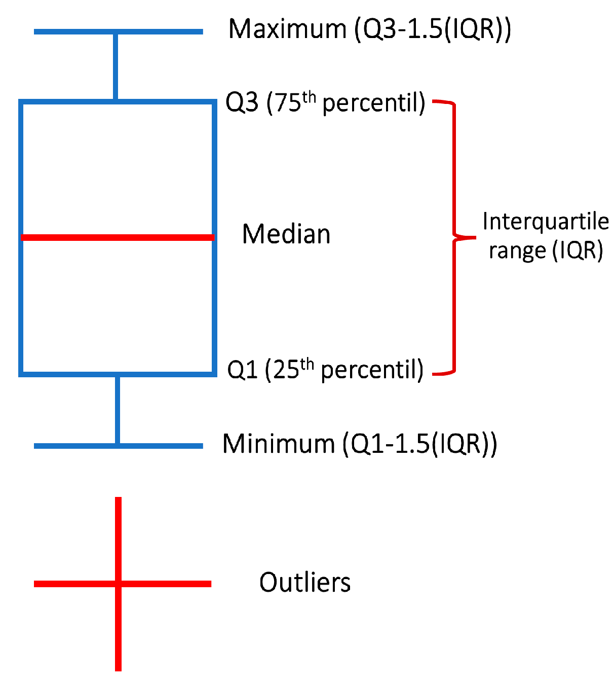
Figure 10.
Box and whisker symbology.
Figure 10.
Box and whisker symbology.
Figure 11.
(a) FRC concentrations on the farthest modes from the initial distribution (node 30). Last day of simulation obtained for GA and PSO. (b) FRC concentrations on the farthest modes from the initial distribution (N = node 34). Last day of simulation obtained for GA and PSO. (c) FRC concentrations on the farthest modes from the initial distribution (node 36). Last day of simulation obtained for GA and PSO.
Figure 12.
CBS location proposed by the PSO simulation in Case 2.
Figure 12.
CBS location proposed by the PSO simulation in Case 2.
Figure 13.
FRC distribution at hour 288 with CBS with fixed pattern dosage of 4 mg/L per hour.
Figure 13.
FRC distribution at hour 288 with CBS with fixed pattern dosage of 4 mg/L per hour.
Figure 14.
Chlorine injection dosage by pattern hour between the limits of 0.2 and 5 mg/L.
Figure 14.
Chlorine injection dosage by pattern hour between the limits of 0.2 and 5 mg/L.
Figure 15.
Pattern time dosage in Case 2 between local regulations.
Figure 15.
Pattern time dosage in Case 2 between local regulations.
Figure 16.
FRC distribution in Case 2 by scheduling hourly dosage pattern obtained in
Figure 15.
Figure 16.
FRC distribution in Case 2 by scheduling hourly dosage pattern obtained in
Figure 15.
Figure 17.
Box and whisker FRC distribution in Case 2 for critical nodes.
Figure 17.
Box and whisker FRC distribution in Case 2 for critical nodes.
Table 1.
Number of CBS distribution and frequency proposed by GA technique, (Statistical GA Location at Case 1).
Table 1.
Number of CBS distribution and frequency proposed by GA technique, (Statistical GA Location at Case 1).
| CBS | CBS Simulation Reached | CBS ID |
|---|
| 2 | 56 | Node 1, Tank |
| 3 | 30 | Node 1, Node 14, Tank |
| 4 | 13 | Node 1, Node 14, Node 29, Tank |
| 5 | 1 | Node 1, Node 29, Node E, Node 32 |
| Total | 100 1 | |
Table 2.
Number of CBS distribution and frequency proposed by PSO, (statistical PSO location at Case 1).
Table 2.
Number of CBS distribution and frequency proposed by PSO, (statistical PSO location at Case 1).
| CBS | CBS Reached | CBS ID |
|---|
| 2 | 71 | Node 1, Tank |
| 3 | 19 | Node 1, Node 14, Tank |
| 4 | 8 | Node 1, Node 14, Node 29, Tank |
| 5 | 2 | Node 1, Node 14, Node 29, (Node E or Node 8) |
| Total | 100 1 | |
Table 3.
Statistical values of FRC (mg/L) from the last 24 h of simulation in all nodes.
Table 3.
Statistical values of FRC (mg/L) from the last 24 h of simulation in all nodes.
| Metaheuristic Technique | Mean | Standard Deviation Mean | Min | Max |
|---|
| GA | 0.64 | 0.25 | 0.20 | 2.24 |
| PSO | 0.53 | 0.43 | 0.20 | 3.87 |
Table 4.
Comparison of the total mass injected by the CBS obtained with GA and PSO with those described in the literature review for Case 1.
Table 4.
Comparison of the total mass injected by the CBS obtained with GA and PSO with those described in the literature review for Case 1.
| Author and Year | Optimization Technique | Selected
Nodes | Mean Dosage (mg/L) | Total Dosage (g/Day) |
|---|
| This paper | GA (Case study 1) | Node 1
Node 25 | 0.79
1.29 | 1762 |
| This paper | PSO (Case study 1) | Node 1
Tank | 1.13
0.76 | 1279 |
| Boccelli et al., 1998 [32] | 1 Linear Programming. Case IV | Link 1 (A)
Link 8 (B)
Link 9 (C)
Link 38 (D)
Link 34 (E)
Link 29 (F) | 318.8 1
4.65 1
2089.6 1
0.01 1
0.6 1
- | 3475 |
| Propato and Uber, 2004 [36] | Linear Least Squares | Link 1 (A)
Link 29 (F) | 0.26
0.22 | 1321 |
| Ayvaz et al., 2018 [37] | Hybrid optimization with solver Harmony Search | Node 2
Node 25 | 0.517
0.349 | 1213 |
Table 5.
Characteristics of critical nodes in Case 2.
Table 5.
Characteristics of critical nodes in Case 2.
| Nodes ID | Elevation (m) | Node Demand (L/s) | Pressure (m) |
|---|
| ‘DQ512’ | 2071.38 | 0.04 | 31.63 |
| ‘QD106’ | 2021.63 | 0.02 | 43.11 |
| ‘DQ938’ | 2059.97 | 0.06 | 17.87 |
| ‘800’ | 1998.83 | 0.06 | 62.68 |
| ‘QD238’ | 1966.00 | 0.22 | 94.84 |
| ‘DQ17’ | 2035.64 | 0.14 | 20.86 |
Table 6.
Statistical values of FRC (mg/L) from the last 24 h of simulation in all nodes.
Table 6.
Statistical values of FRC (mg/L) from the last 24 h of simulation in all nodes.
| Metaheuristic Technique | Mean | Std Deviation Mean | Min | Max | Hours Upper 0.2 |
|---|
| PSO | 0.71 | 0.25 | 0 | 1.5 | 95.85% |
| Publisher’s Note: MDPI stays neutral with regard to jurisdictional claims in published maps and institutional affiliations. |
© 2021 by the authors. Licensee MDPI, Basel, Switzerland. This article is an open access article distributed under the terms and conditions of the Creative Commons Attribution (CC BY) license (https://creativecommons.org/licenses/by/4.0/).


 ,
, 


