
Comparison of AC and DC Nanogrid for Office Buildings with EV Charging, PV and Battery Storage


Abstract
:1. Introduction
1.1. Objective
1.2. Literature Review
1.3. Research Contribution
- System efficiency: System efficiency correlates to the system electrical energy autarky (EEA) and the annual saving. EEA indicates the independency of the system to the electricity grid without taking into account the heat load demand and fuel consumption [22]. More efficient system means that there is less losses occurring in the system’s components (e.g., converters, cables, etc.). Therefore, more energy can be utilized for the loads and less energy is required from external grid. In the other case, when the PV generates more energy than demanded, there will be more excess energy that can be sold to the grid.
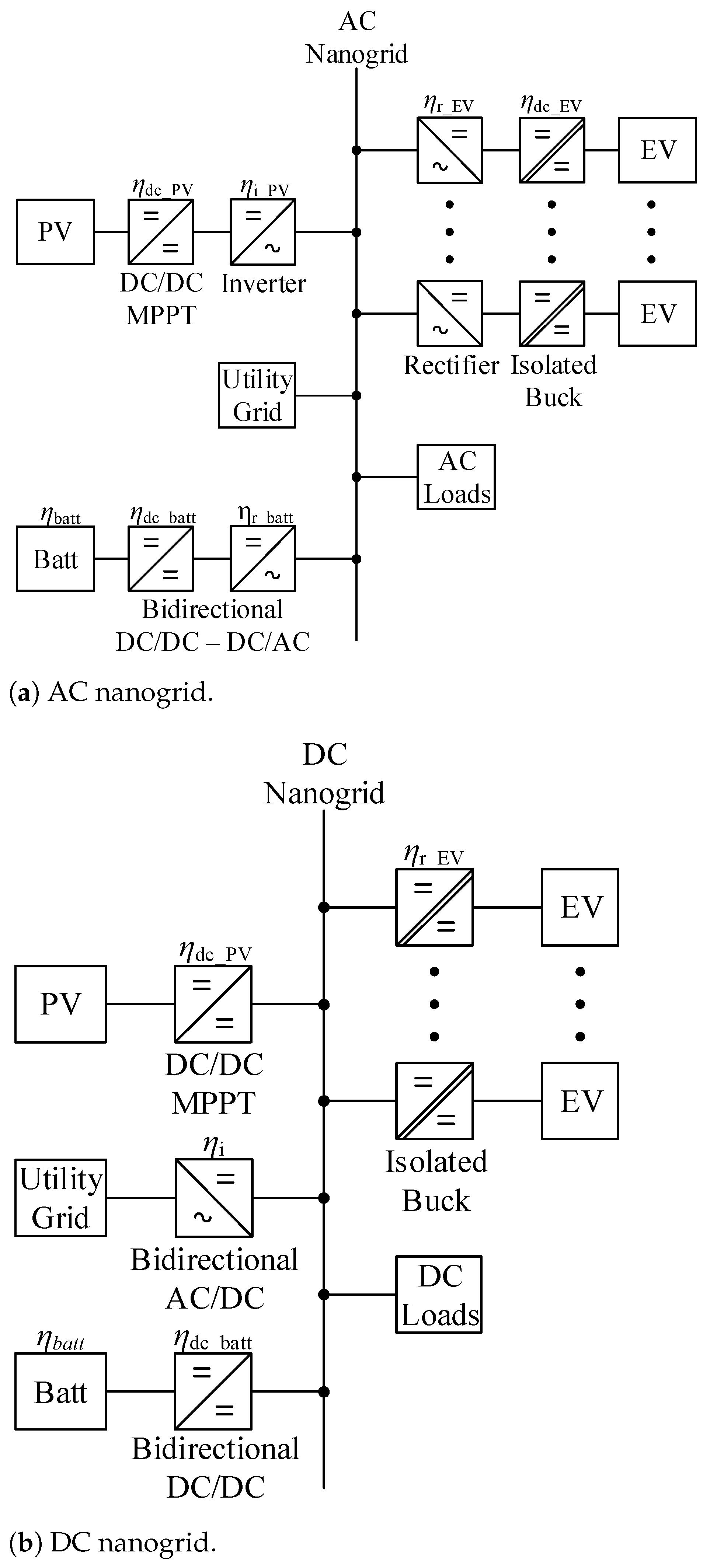
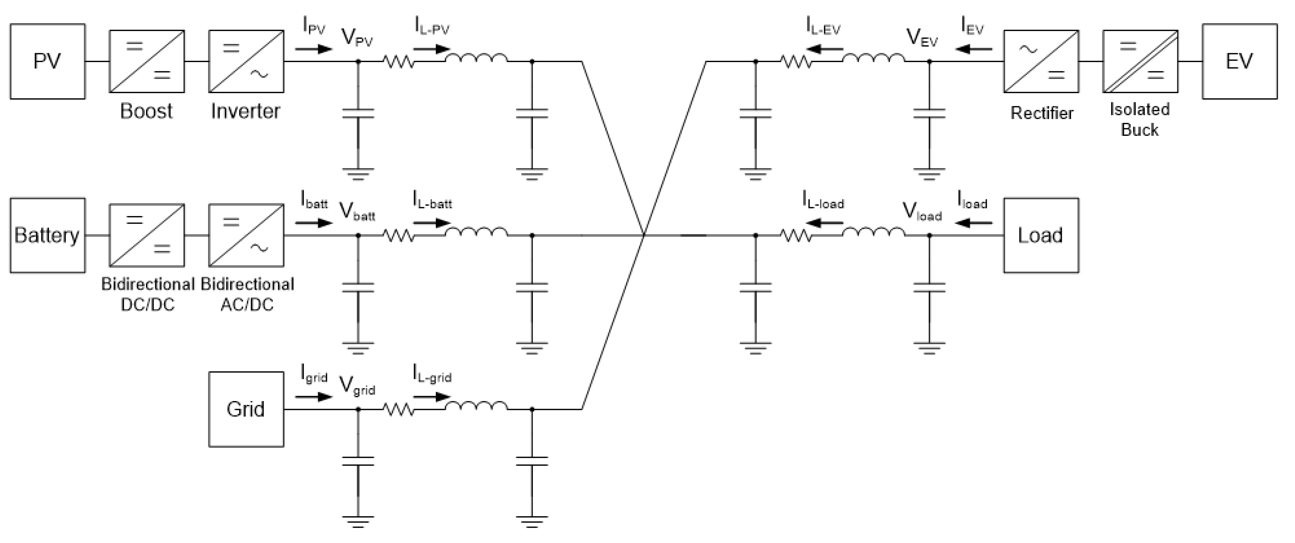
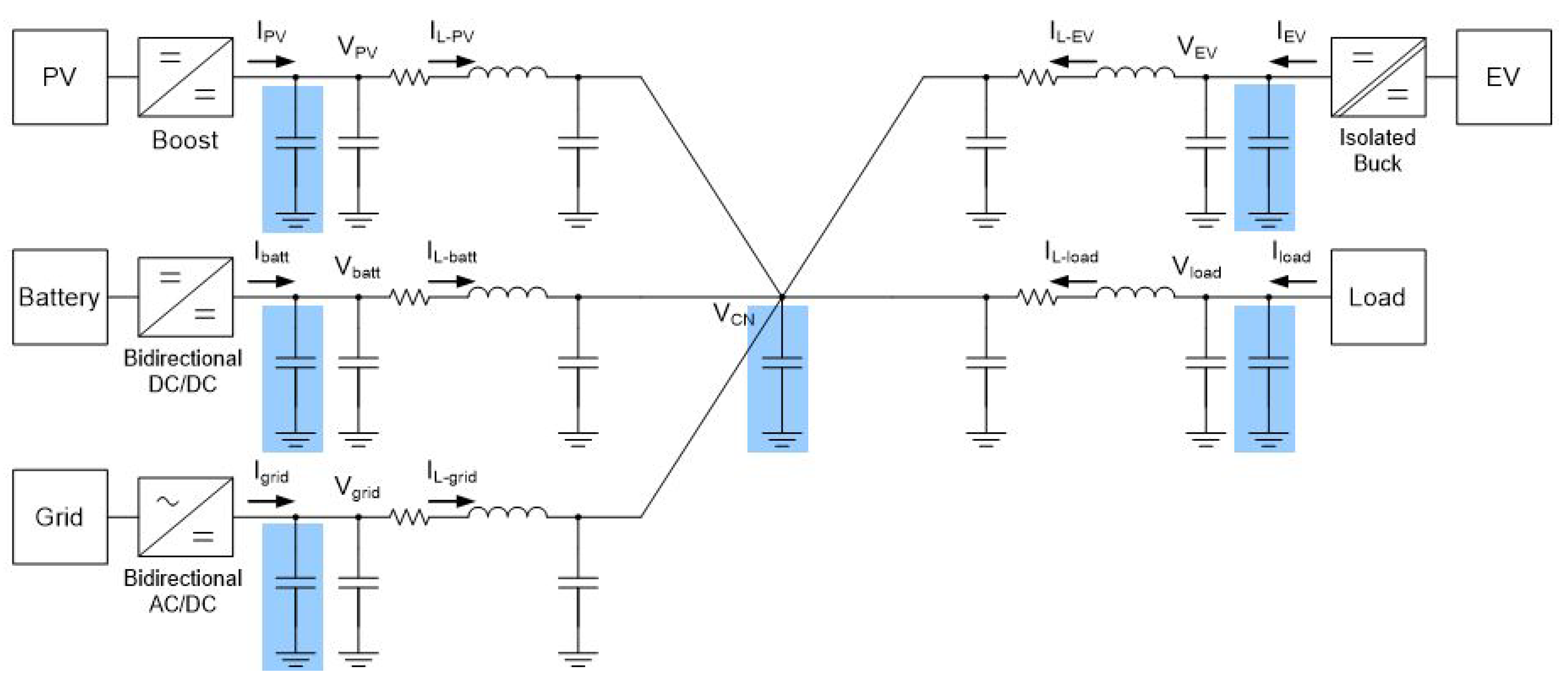
- Control:Figure 1 shows two types of building’s interconnection with PV, EV, battery, loads, and grid. In AC nanogrid, as shown in Figure 1a, the utility grid is directly connected to the nanogrid. Therefore, changes in demand or production in the office will not affect the AC nanogrid since the AC grid is assumed as a very stable source.Even though the system can be considered to be very stable; voltage, frequency, and reactive power have to be controlled in order to maintain the stability of the system. DC nanogrid, as shown in Figure 1b, is more challenging in terms of control. Although there is no frequency and reactive power issues, the AC grid is not directly connected to the nanogrid, but through an AC/DC bidirectional converter. This converter plays a significant role to maintain the stability of the DC nanogrid.
- Protection and Safety: Different nature of AC and DC currents necessities different protection mechanism for the two systems. The presence of frequency and zero crossing in AC nanogrid makes the system easier to be dealt with during a fault condition. The inductance of the cables within the system will lower the fault current and the zero crossing helps extinguishing the arc automatically. However, absence of current zero crossing in DC nanogrid makes both series and parallel electric arcs a concern [23,24]. During short circuits, the fault current in DC is higher and the absence of zero crossing makes the arc persist which is hazardous.
1.4. Paper Organization
2. System Description
2.1. System Architecture
2.2. System Size and Power Profiles
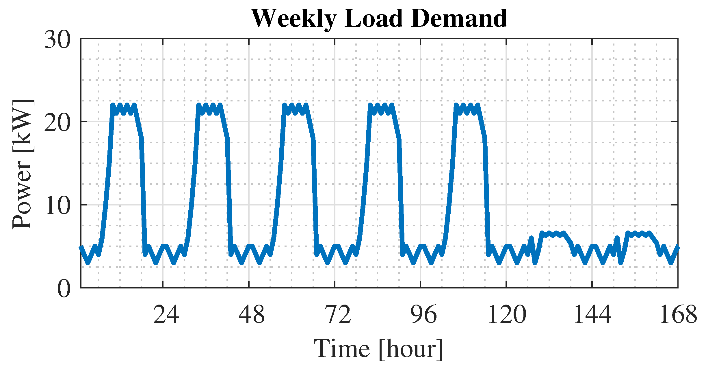
2.2.1. Office loads
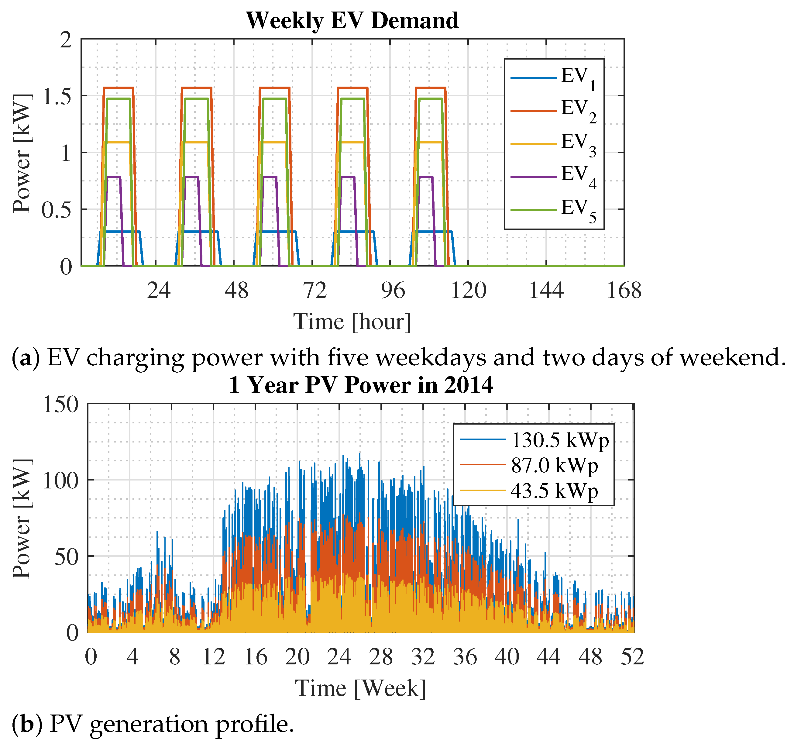
2.2.2. EV Charging Profile
2.2.3. PV Generation Profile
3. Comparison of Average Operating Efficiency
3.1. Assumptions
- The battery ESS is constrained between 10% to 90% depth of discharge.
- The efficiency of each conversion step is set to a vlue of 98%.
- Conduction losses associated with power distribution in the AC nanogrid are represented with efficiency = 99%. This includes power losses in cables, protection devices, busbars, and contact point resistances.
- While the PV data for an entire year is considered to account for the seasonal/daily variation in power profile, weekdays-weekends load and EV profile used over the year for the presented results. Therefore some deviation due to seasonal variation is expected, which is not considered in this paper.
3.2. AC and DC Conduction Losses
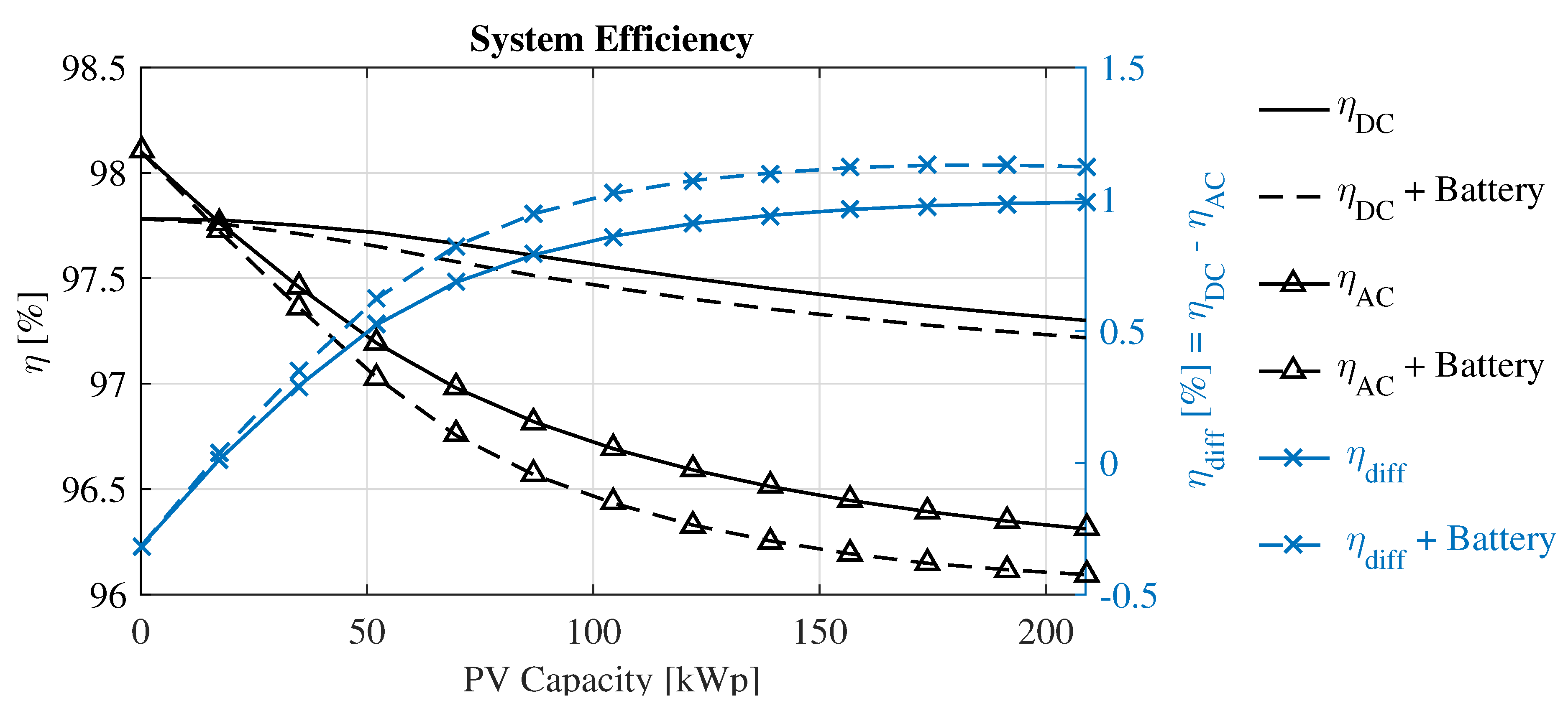
3.3. System Efficiency
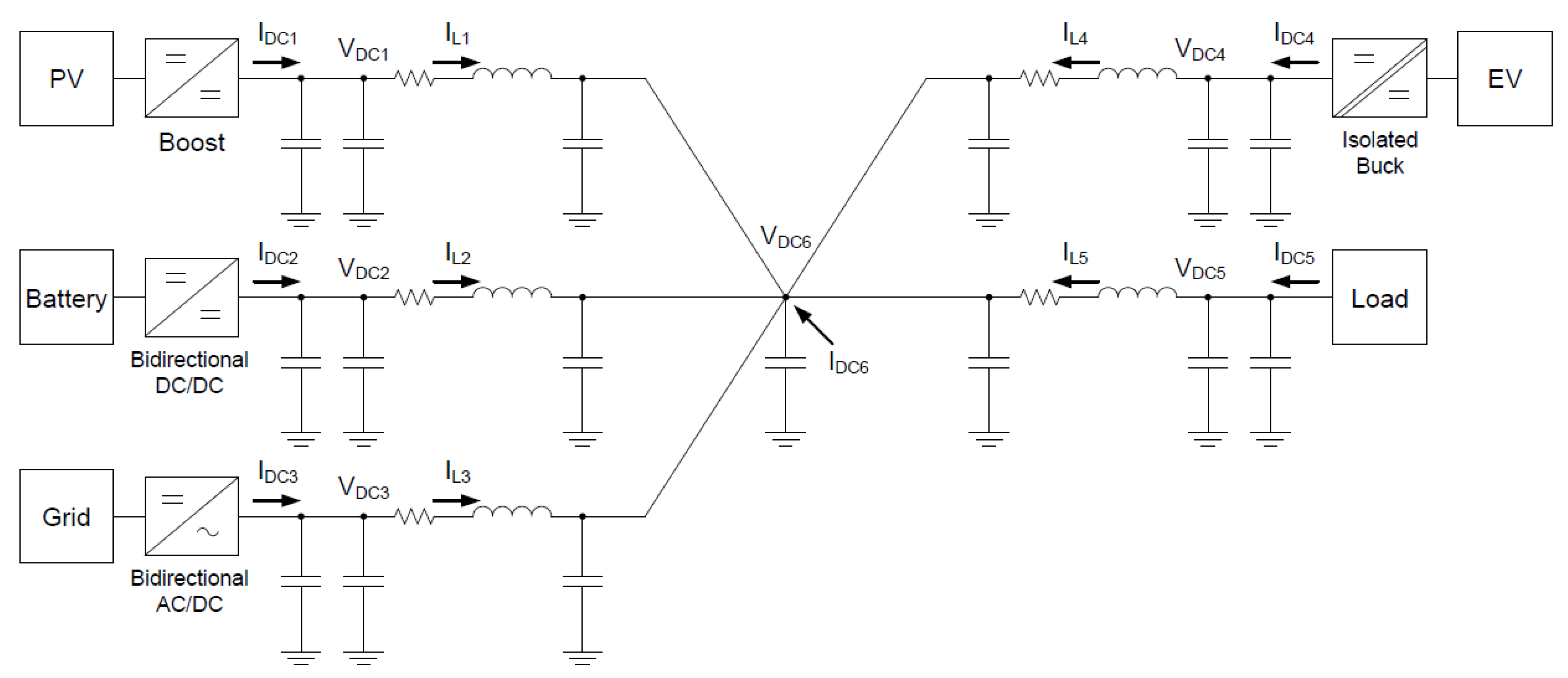
3.3.1. Power Balance Equations
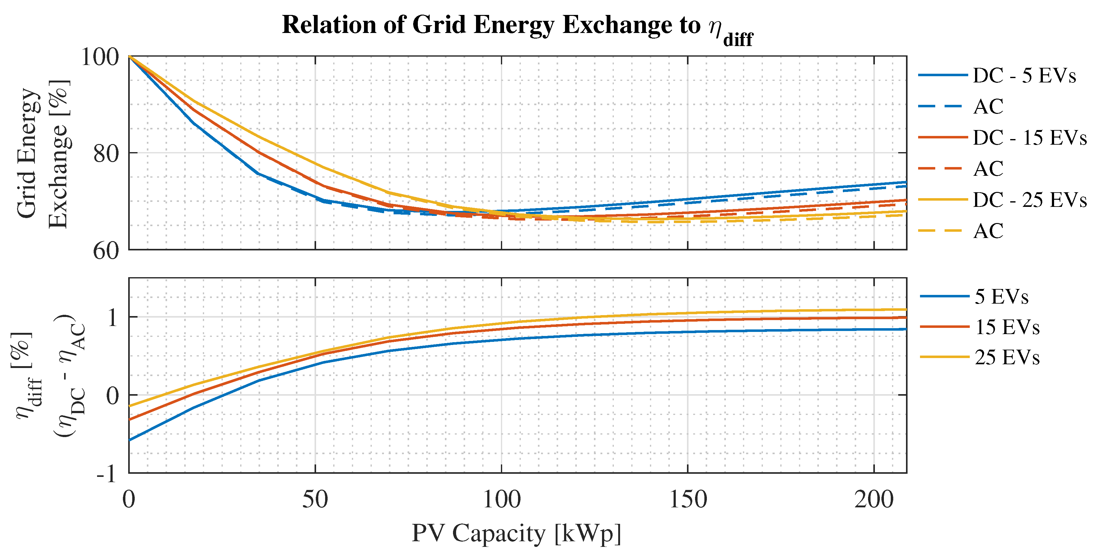
3.3.2. Sensitivity Analysis with Varying PV and EV Energy
3.3.3. Impact of battery
4. Control and Protection Comparison
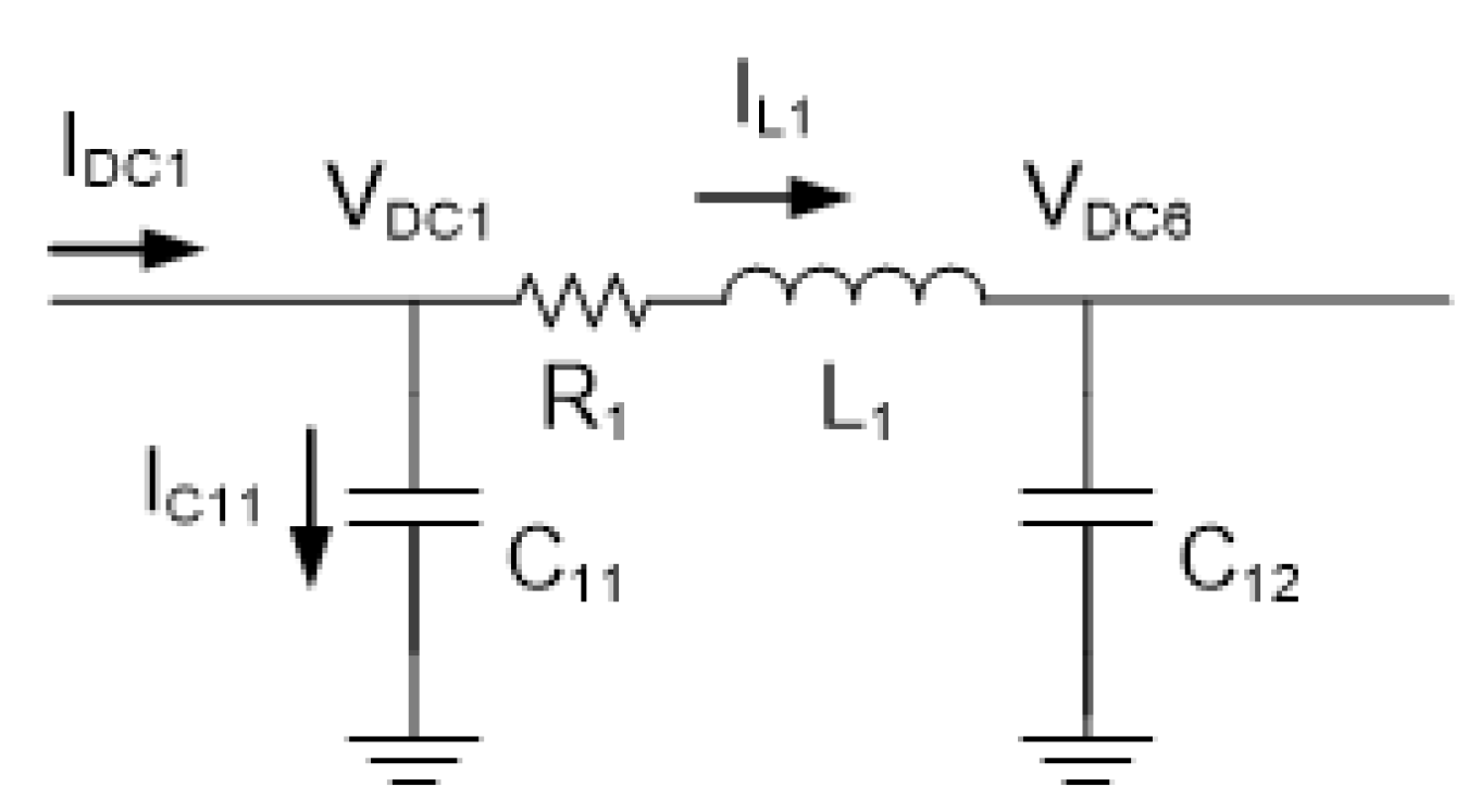
4.1. System Model
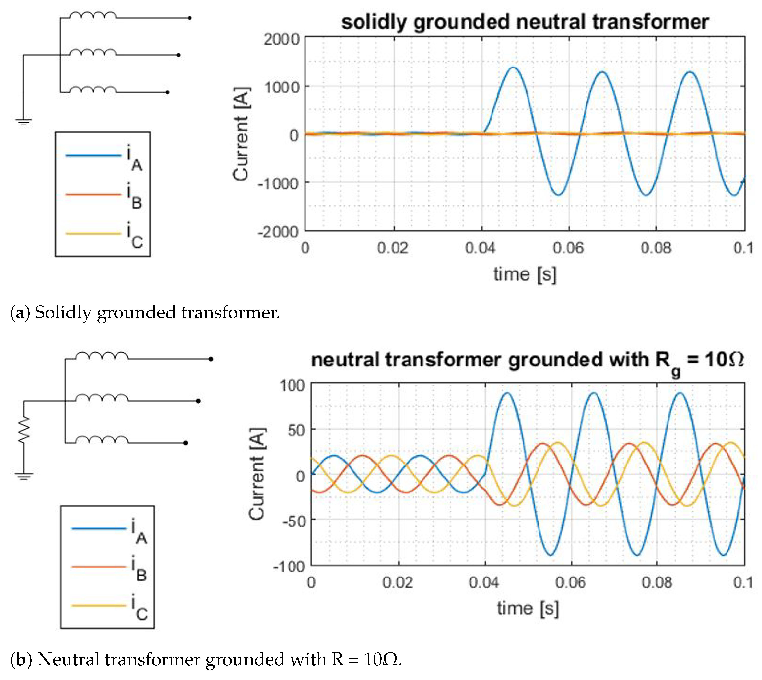
4.2. AC Nanogrid Results
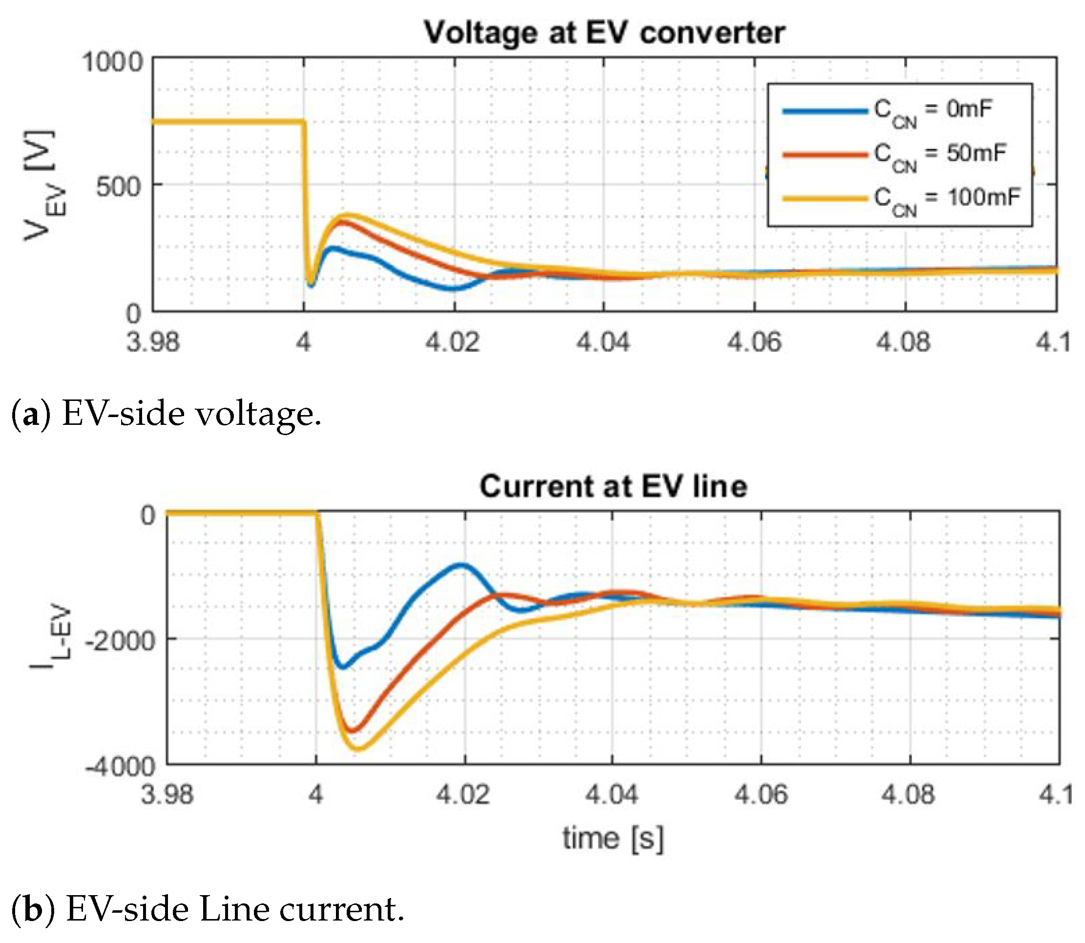
4.3. DC Nanogrid Results
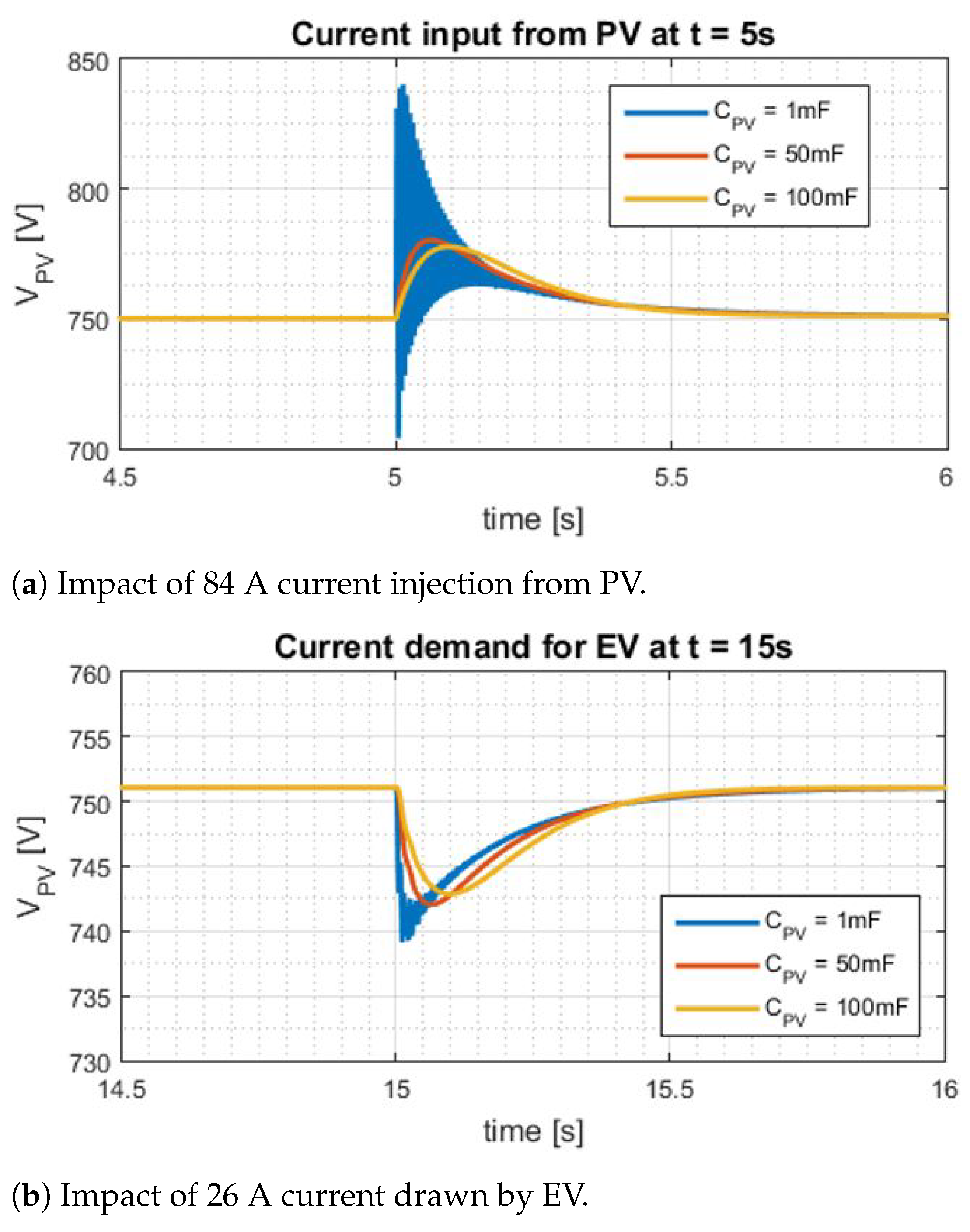
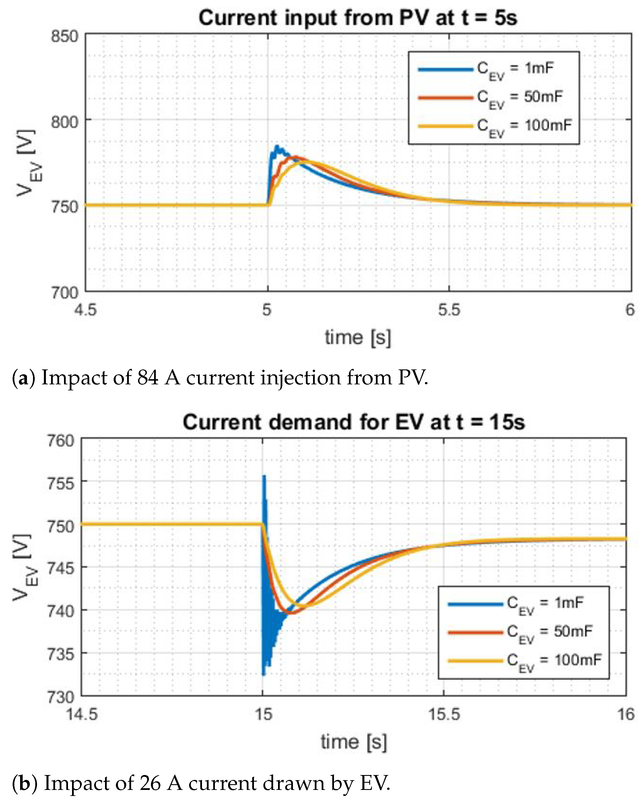
4.3.1. Power Variation
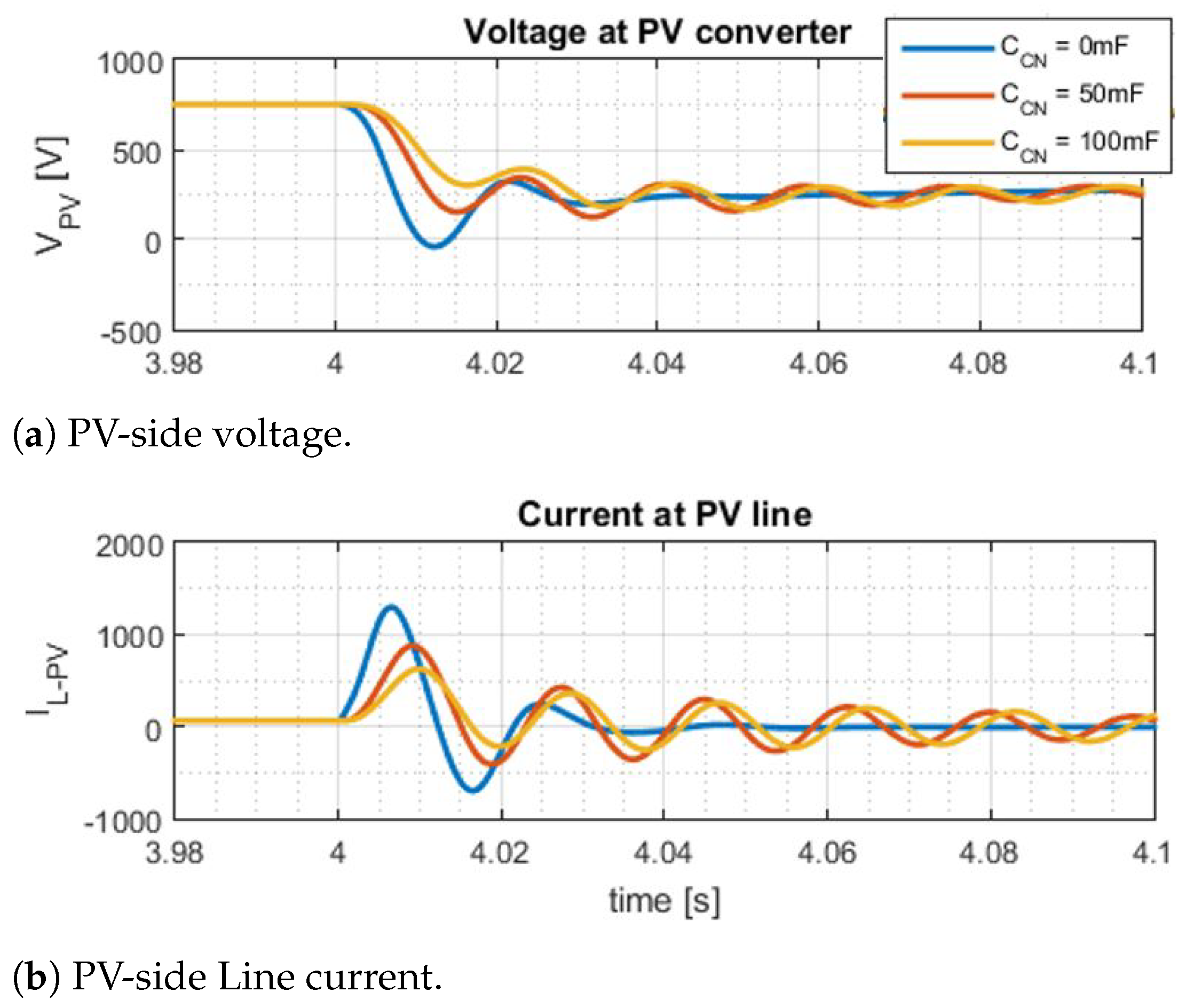
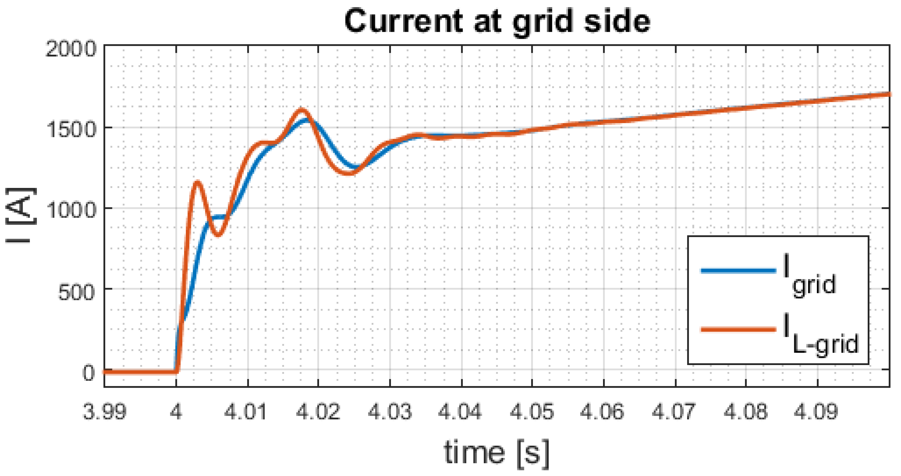
4.3.2. DC Faults
5. Conclusions
- Fast fault interruption. As observed in Section 4.3.2, fast fault interruption time is necessary for DC interconnection. Currently, solid state switches is used for fast interruption and it is more expensive than the conventional circuit breakers. Finding a method that could provide fast interruption and economically viable will make DC nanogrid more attractive.
- Monopolar vs. Bipolar. The behavior of bipolar DC system and the impact of full-rated voltage and neutral line imbalance to the appliances have not been covered in this study.
- Addressing high current during start-up or fault. In DC system, the bidirectional AC/DC converter which connects the grid is important because it regulates the system. During start-up or fault, this converter has to withstand a high current before the fault is isolated. Therefore, attenuating the current or improving the capability of bidirectional AC/DC is important.
Author Contributions
Funding
Institutional Review Board Statement
Informed Consent Statement
Conflicts of Interest
Appendix A

| No | Components | Peak Current [A] | Cable Type | |
|---|---|---|---|---|
| AC | DC | |||
| 1 | PV | 90.93 | 84.00 | AWG 2 |
| 2 | ESS | 33.05 | 30.53 | AWG 8 |
| 3 | Grid | 60.04 | 55.47 | AWG 4 |
| 4 | Office appliances | 31.75 | 29.33 | AWG 8 |
| 5 | EV | 28.29 | 26.13 | AWG 10 |
| No | Components | Cable’s Specifications | ||
|---|---|---|---|---|
| Total R [mΩ] | Total H [μH] | Total C [pF] | ||
| 1 | PV | 25.63 | 876.1 | 1118 |
| 2 | ESS | 30.91 | 247.5 | 237.6 |
| 3 | Grid | 12.22 | 233.5 | 286.2 |
| 4 | Office appliances | 103.1 | 945.5 | 792.1 |
| 5 | EV | 65.54 | 351.28 | 339.12 |
References
- Dincer, I. Renewable energy and sustainable development: A crucial review. Renew. Sustain. Energy Rev. 2000, 4, 157–175. [Google Scholar] [CrossRef]
- IRENA. Renewable Energy Capacity Statistics 2015; Technical Report; IRENA: Abu Dhabi, United Arab Emirates, 2015. [Google Scholar] [CrossRef]
- REN21. Renewables 2015 Global Status Report; Technical Report; L Renewable Energy Policy Network for the 21st Century: Paris, France, 2015. [Google Scholar]
- Shekhar, A.; Prasanth, V.; Bauer, P.; Bolech, M. Economic viability study of an on-road wireless charging system with a generic driving range estimation method. Energies 2016, 9, 76. [Google Scholar] [CrossRef] [Green Version]
- Mouli, G.C.; Bauer, P.; Zeman, M. System design for a solar powered electric vehicle charging station for workplaces. Appl. Energy 2016, 168, 434–443. [Google Scholar] [CrossRef] [Green Version]
- Chandra Mouli, G.R.; Kefayati, M.; Baldick, R.; Bauer, P. Integrated PV Charging of EV Fleet Based on Energy Prices, V2G, and Offer of Reserves. IEEE Trans. Smart Grid 2019, 10, 1313–1325. [Google Scholar] [CrossRef]
- Venugopal, P.; Shekhar, A.; Visser, E.; Scheele, N.; Mouli, G.R.C.; Bauer, P.; Silvester, S. Roadway to self-healing highways with integrated wireless electric vehicle charging and sustainable energy harvesting technologies. Appl. Energy 2018, 212, 1226–1239. [Google Scholar] [CrossRef]
- Deboever, J.; Peppanen, J.; Maitra, A.; Damato, G.; Taylor, J.; Patel, J. Energy Storage as a Non-Wires Alternative for Deferring Distribution Capacity Investments. In Proceedings of the 2018 IEEE/PES Transmission and Distribution Conference and Exposition (T D), Denver, CO, USA, 16–19 April 2018; pp. 1–5. [Google Scholar] [CrossRef]
- Faisal, M.; Hannan, M.A.; Ker, P.J.; Hussain, A.; Mansor, M.B.; Blaabjerg, F. Review of Energy Storage System Technologies in Microgrid Applications: Issues and Challenges. IEEE Access 2018, 6, 35143–35164. [Google Scholar] [CrossRef]
- Yang, Y.; Bremner, S.; Menictas, C.; Kay, M. Battery energy storage system size determination in renewable energy systems: A review. Renew. Sustain. Energy Rev. 2018, 91, 109–125. [Google Scholar] [CrossRef]
- Dragicevic, T.; Wheeler, P.; Blaabjerg, F. (Eds.) DC Distribution Systems and Microgrids, 1st ed.; Institution of Engineering and Technology: London, UK, 2018; Volume 1. [Google Scholar] [CrossRef]
- Dragičević, T.; Lu, X.; Vasquez, J.C.; Guerrero, J.M. DC Microgrids-Part II: A Review of Power Architectures, Applications, and Standardization Issues. IEEE Trans. Power Electron. 2016, 31, 3528–3549. [Google Scholar] [CrossRef] [Green Version]
- Emhemed, A.; Burt, G. The effectiveness of using IEC61660 for characterising short-circuit currents of future low voltage DC distribution networks. In Proceedings of the 22nd International Conference and Exhibition on Electricity Distribution (CIRED 2013), Stockholm, Sweden, 10–13 June 2013; pp. 1–4. [Google Scholar] [CrossRef] [Green Version]
- Saputra, F.W.Y.; Aripriharta.; Fadlika, I.; Mufti, N.; Wibowo, K.H.; Jong, G.J. Efficiency Comparison between DC and AC Grid Toward Green Energy In Indonesia. In Proceedings of the 2019 IEEE International Conference on Automatic Control and Intelligent Systems (I2CACIS), Shah Alam, Malaysia, 29 June 2019; pp. 129–134. [Google Scholar] [CrossRef]
- Mackay, L.; van der Blij, N.H.; Ramirez-Elizondo, L.; Bauer, P. Toward the Universal DC Distribution System. Electr. Power Components Syst. 2017, 45, 1032–1042. [Google Scholar] [CrossRef] [Green Version]
- Mouli, G.R.C.; Bauer, P.; Zeman, M. Comparison of system architecture and converter topology for a solar powered electric vehicle charging station. In Proceedings of the 2015 9th International Conference on Power Electronics and ECCE Asia (ICPE-ECCE Asia), Seoul, Korea, 1–5 June 2015; pp. 1908–1915. [Google Scholar] [CrossRef] [Green Version]
- Meliopoulos, A.P.S.; Martin, M.A. Calculation of secondary cable losses and ampacity in the presence of harmonics. IEEE Trans. Power Deliv. 1992, 7, 451–459. [Google Scholar] [CrossRef]
- Dastgeer, F.; Kalam, A. Efficiency comparison of DC and AC distribution systems for distributed generation. In Proceedings of the 2009 Australasian Universities Power Engineering Conference, Adelaide, Australia, 27–30 September 2009; pp. 1–5. [Google Scholar]
- ABB. Technical Application Papers No.14 Faults in LVDC Microgrids with Front-End Converters; ABB: Zürich, Switzerland, 2015. [Google Scholar]
- Estes, H.B.; Kwasinski, A.; Hebner, R.E.; Uriarte, F.M.; Gattozzi, A.L. Open series fault comparison in AC amp; DC micro-grid architectures. In Proceedings of the 2011 IEEE 33rd International Telecommunications Energy Conference (INTELEC), Amsterdam, The Netherlands, 9–13 October 2011; pp. 1–6. [Google Scholar] [CrossRef]
- Justo, J.J.; Mwasilu, F.; Lee, J.; Jung, J.W. AC-microgrids versus DC-microgrids with distributed energy resources: A review. Renew. Sustain. Energy Rev. 2013, 24, 387–405. [Google Scholar] [CrossRef]
- Barco, H.E.C. Hybrid Renewable Energy Systems, Control Strategy & Project Evaluation. Ph.D. Thesis, Department Intelligent Electrical power Grids, Delft, The Netherlands, 2013. [Google Scholar]
- Shekhar, A.; Ramírez-Elizondo, L.; Bandyopadhyay, S.; Mackay, L.; Bauera, P. Detection of series arcs using load side voltage drop for protection of low voltage DC systems. IEEE Trans. Smart Grid 2017, 9, 6288–6297. [Google Scholar] [CrossRef] [Green Version]
- Liu, Z.; Shekhar, A.; Ramírez-Elizondo, L.; Bauer, P. Characterization of series arcs in LVdc microgrids. In Proceedings of the 2017 IEEE Second International Conference on DC Microgrids (ICDCM), Nuremburg, Germany, 27–29 June 2017; pp. 297–301. [Google Scholar]
- Gerber, D.L.; Vossos, V.; Feng, W.; Marnay, C.; Nordman, B.; Brown, R. A simulation-based efficiency comparison of AC and DC power distribution networks in commercial buildings. Appl. Energy 2018, 210, 1167–1187. [Google Scholar] [CrossRef] [Green Version]
- Mocanu, E.; Nguyen, P.H.; Gibescu, M.; Kling, W.L. Comparison of machine learning methods for estimating energy consumption in buildings. In Proceedings of the 2014 International Conference on Probabilistic Methods Applied to Power Systems (PMAPS), Durham, UK, 7–10 July 2014; pp. 1–6. [Google Scholar] [CrossRef] [Green Version]
- Mackay, L.; Ramirez-Elizondo, L.; Bauer, P. DC ready devices—Is redimensioning of the rectification components necessary? In Proceedings of the 16th International Conference on Mechatronics—Mechatronika 2014, Brno, Czech Republic, 3–5 December 2014; pp. 1–5. [Google Scholar]
- Wu, T.; Chen, Y.; Yu, G.; Chang, Y. Design and development of dc-distributed system with grid connection for residential applications. In Proceedings of the 8th International Conference on Power Electronics—ECCE Asia, Jeju, Korea, 30 May–3 June 2011; pp. 235–241. [Google Scholar]
- Wunder, B.; Ott, L.; Szpek, M.; Boeke, U.; Weiß, R. Energy efficient DC-grids for commercial buildings. In Proceedings of the 2014 IEEE 36th International Telecommunications Energy Conference (INTELEC), Vancouver, BC, Canada, 28 September–2 October 2014; pp. 1–8. [Google Scholar]
- Torreglosa, J.P.; García-Triviño, P.; Fernàndez-Ramirez, L.M.; Jurado, F. Decentralized energy management strategy based on predictive controllers for a medium voltage direct current photovoltaic electric vehicle charging station. Energy Convers. Manag. 2016, 108, 1–13. [Google Scholar] [CrossRef]
- Baboli, P.T.; Bahramara, S.; Moghaddam, M.P.; Haghifam, M.R. A mixed-integer linear model for optimal operation of hybrid AC-DC microgrid considering Renewable Energy Resources and PHEVs. In Proceedings of the 2015 IEEE Eindhoven PowerTech, Eindhoven, The Netherlands, 29 June–2 July 2015; pp. 1–5. [Google Scholar] [CrossRef]
- Sulaeman, I.; Vega-Garita, V.; Mouli, G.R.C.; Narayan, N.; Ramirez-Elizondo, L.; Bauer, P. Comparison of PV-battery architectures for residential applications. In Proceedings of the 2016 IEEE International Energy Conference (ENERGYCON), Leuven, Belgium, 4–8 April 2016; pp. 1–7. [Google Scholar] [CrossRef] [Green Version]
- Van der Sluis, L. Transients in Power Systems; John Wiley & Sons, LTD.: Hoboken, NJ, USA, 2001. [Google Scholar]
- Panduit. Electrical Wire Sizes Selection Guide. 2011. Available online: http://www.panduit.com/heiler/SelectionGuides/WW-WASG03%20Electrical%20Wire%20Sizes-WEB%207-7-11.pdf (accessed on 9 September 2021).
- Rosa, E.B. The Self and Mutual Inductances of Linear Conductors. In Bulletin of the Bureau of Standards; Government Printing Office: Washington, DC, USA, 1908; Volume 4, pp. 301–344. [Google Scholar]
- Noriega, B.E.; Pinto, R.T.; Bauer, P. Sustainable DC-microgrid control system for electric-vehicle charging stations. In Proceedings of the 2013 15th European Conference on Power Electronics and Applications (EPE), Lille, France, 2–6 September 2013; pp. 1–10. [Google Scholar] [CrossRef]
- Carminati, M.; Ragaini, E.; Tironi, E. DC and AC ground fault analysis in LVDC microgrids with energy storage systems. In Proceedings of the 2015 IEEE 15th International Conference on Environment and Electrical Engineering (EEEIC), Rome, Italy, 10–13 June 2015; pp. 1047–1054. [Google Scholar] [CrossRef]
- Schroder, S.; Meyer, C.; Doncker, R.W.D. Solid-state circuit breakers and current-limiting devices for medium-voltage systems. In Proceedings of the VIII IEEE International Power Electronics Congress, Guadalajara, Mexico, 20–24 October 2002; pp. 91–95. [Google Scholar] [CrossRef]
- Meyer, C.; Schroder, S.; Doncker, R.W.D. Design of solid-state circuit breakers for medium-voltage systems. In Proceedings of the 2003 IEEE PES Transmission and Distribution Conference and Exposition (IEEE Cat. No.03CH37495), Dallas, TX, USA, 7–12 September 2003; Volume 2, pp. 798–803. [Google Scholar] [CrossRef]


| Power Flows | Conversion Steps | Power Flows | Conversion Steps | ||
|---|---|---|---|---|---|
| AC | DC | AC | DC | ||
| PV → load | 2 | 1 | Batt → load | 2 | 1 |
| PV → EV | 4 | 2 | Batt → EV | 4 | 2 |
| PV → grid | 2 | 2 | Grid → load | - | 1 |
| PV → batt | 4 | 2 | Grid → EV | 2 | 2 |
| Capacitor on Components’ Side | Required Capacitor Size |
|---|---|
| PV | 11 mF |
| ESS | 3 mF |
| EV | 3 mF |
| grid | 3 mF |
| Fault at | Required Interruption Time [ms] | ||
|---|---|---|---|
| mF | mF | mF | |
| PV | 3 | 6.5 | 9 |
| EV | 2 | 5 | 6.2 |
| ESS | 0.5 | 4 | 6 |
| Office appliances | 3 | 7.5 | 11 |
| Grid | 0.3 | 3.3 | 5.1 |
| AC Nanogrid | DC Nanogrid | |
|---|---|---|
| Presence of capacitors | Present only due to parasitic connection with earth. Does not give significant effect on system response | Required for control and stability purpose. Lowers voltage oscillations during power mismatch. Highly affect the fault current and voltage response. Bigger capacitors improve the system response but it causes high start-up, fault transient current, and more expensive. |
| Fault interruption time | Required time: 40 ms. The longer it takes to interrupt the fault, the higher the fault current. | Required time: 4 ms. The longer the fault’s interruption, not only the high current, but also the high voltage rise will occur once the fault is isolated. |
| Arc protection devices | Not required | Highly required due to the absence of zero crossing. |
| Suitable protection devices | Fuses and mechanical circuit breaker | Solid state switch. Additional L can be used to have lower voltage drop rate but it reduces the system response. |
| Fault current | ||
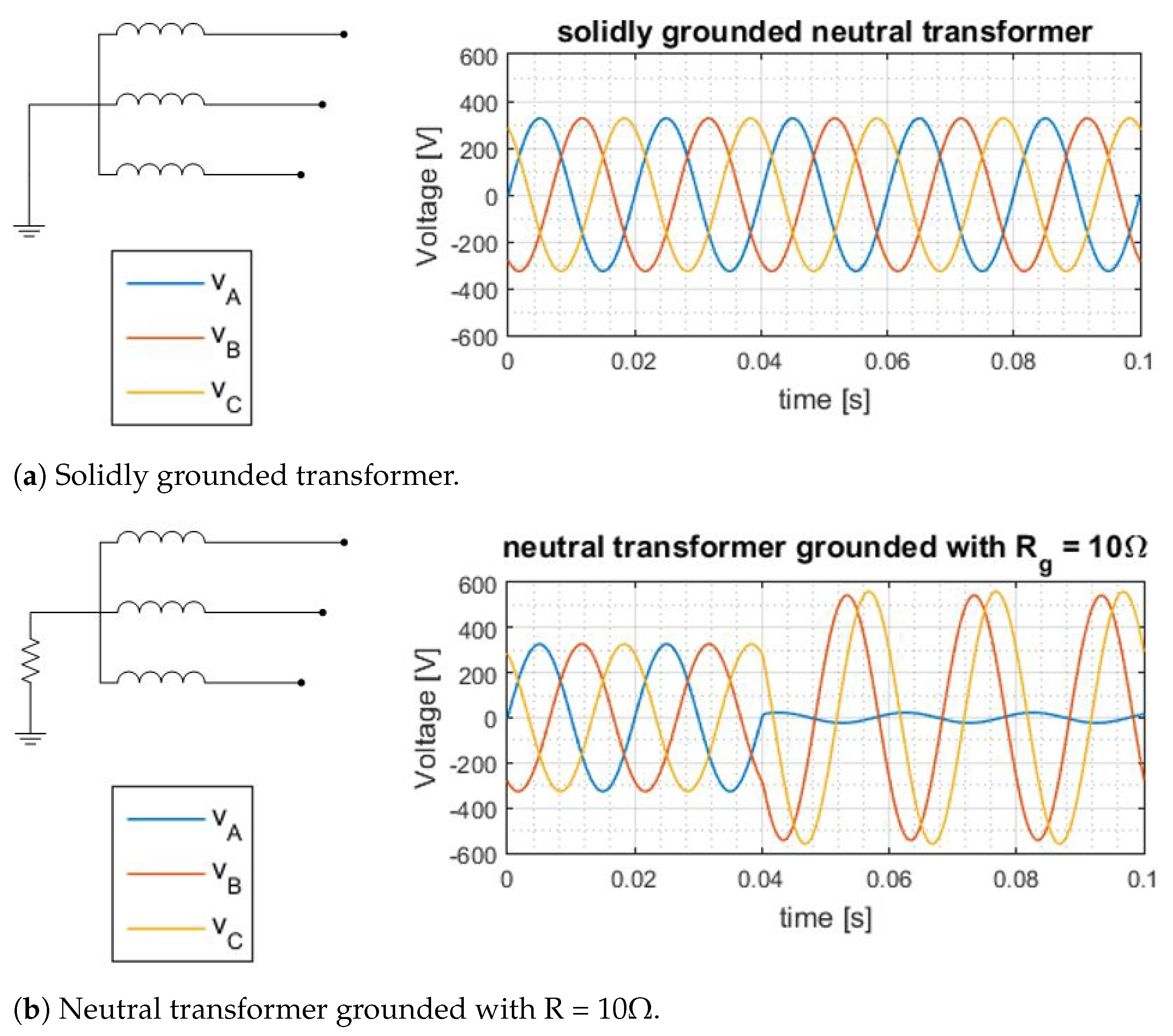
| Transient fault current | The transient peak is not present in AC side if the neutral transformer is grounded. | Transient current always present regardless of the grounding strategy and highly dependent on the capacitors’ size |
| AC Nanogrid | DC Nanogrid | |
|---|---|---|
| System efficiency | Higher at high grid energy exchange and EV demands are less dominant than office appliances. | Higher at low grid energy exchange and EV demands are more dominant than office appliances. |
| Impact of ESS | More losses due to more conversion steps when more excess PV is stored in ESS. | Similar trend with AC nanogrid but lower losses due to lower conversion steps to ESS. |
| Control and protection | Transient fault current depends on transformer grounding, lower fault current. | More complex, may require buffer capacitor and fast interruption protection device. |
Publisher’s Note: MDPI stays neutral with regard to jurisdictional claims in published maps and institutional affiliations. |
© 2021 by the authors. Licensee MDPI, Basel, Switzerland. This article is an open access article distributed under the terms and conditions of the Creative Commons Attribution (CC BY) license (https://creativecommons.org/licenses/by/4.0/).
Share and Cite
Sulaeman, I.; Chandra Mouli, G.R.; Shekhar, A.; Bauer, P. Comparison of AC and DC Nanogrid for Office Buildings with EV Charging, PV and Battery Storage. Energies 2021, 14, 5800. https://doi.org/10.3390/en14185800
Sulaeman I, Chandra Mouli GR, Shekhar A, Bauer P. Comparison of AC and DC Nanogrid for Office Buildings with EV Charging, PV and Battery Storage. Energies. 2021; 14(18):5800. https://doi.org/10.3390/en14185800
Chicago/Turabian StyleSulaeman, Ilman, Gautham Ram Chandra Mouli, Aditya Shekhar, and Pavol Bauer. 2021. "Comparison of AC and DC Nanogrid for Office Buildings with EV Charging, PV and Battery Storage" Energies 14, no. 18: 5800. https://doi.org/10.3390/en14185800
APA StyleSulaeman, I., Chandra Mouli, G. R., Shekhar, A., & Bauer, P. (2021). Comparison of AC and DC Nanogrid for Office Buildings with EV Charging, PV and Battery Storage. Energies, 14(18), 5800. https://doi.org/10.3390/en14185800