Investigation on Bubble Diameter Distribution in Upward Flow by the Two-Fluid and Multi-Fluid Models

Abstract

Bubble flow can be simulated by the two-fluid model and the multi-fluid model based on the Eulerian method. In this paper, the gas phase was further divided into several groups of dispersed phases according to the diameter by using the Eulerian-Eulerian (E-E) multi-fluid model. The diameters of bubbles in each group were considered to be the same, and their distributions were reorganized according to a specific probability density function. The experimental data of two kinds of bubble flow with different characteristics were used to verify the model. With the help of the open-source CFD software, OpenFOAM-7.x (OpenFOAM-7.0, produced by OpenFOAM foundation, Reading, England), the influences of the group number, the probability distribution function, and the parameters of different bubble diameters on the calculation results were studied. Meanwhile, the numerical simulation results were compared with the two-fluid model and the experimental data. The results show that for the bubble flow with the unimodal distribution, both the multi-fluid model and the two-fluid model can obtain the distribution of gas volume fraction along the pipe radius. The calculation results of the multi-fluid model agree with the experimental data, while those of the two-fluid model differ greatly from the experimental data, which verifies the advantage of the multi-fluid model in calculating the distribution of gas volume fraction in the polydisperse bubble flow. Meanwhile, the multi-fluid model can be used to accurately predict the distribution of the parameters of each phase of the bubble flow if the reasonable bubble diameter distribution is provided and the appropriate interphase force calculation model is determined.

1. Introduction

The gas-liquid two-phase flow is a kind of fluid flow that exists widely in different industries such as energy, water conservancy, and chemical industry. The classical E-E two-fluid model is commonly used to describe the movement of bubble flow. This model treats the gas phase as a single phase and takes the average bubble diameter as that of the whole [1,2]. This method is effective only when the gas volume fraction is low, the turbulence effect is small, and the bubble diameter is uniform [3,4,5]. However, many experimental studies on bubble flows have shown that, when polydispersity is significant, bubbles tend to migrate at different velocities depending on their size [6,7]. So, it is not appropriate to use the two-fluid model to describe the bubble flow in this condition, simply because the movement of bubbles with polydispersity and the forces on them are different. The research of Hibiki T. et al. [8] and Rzehak R. et al. [9] suggested that the lift force a bubble receives is directly related to its diameter. Therefore, the distribution of gas volume fraction of bubbles with significant polydispersity has different characteristics: bubbles with large diameters converge toward the center, while those with small diameter converge toward the wall.

In engineering practice, the bubble flow in a mono-dispersed system is rare, but the bubble flow in a polydisperse system is quite common. Therefore, it is important to study the latter. The adoption of the classical E-E two-fluid model has an obvious limitation. It requires the reorganization of the bubble diameters into several groups according to a specific probability density function, and the movement of bubbles in each group has to be described. While the E-E multi-fluid model can be used to calculate the flow field of the polydisperse bubble flow, the accurate distribution of the radial gas volume fraction along a section in the flow direction can be obtained.

Researchers have studied the calculation of polydisperse turbulent bubbles, such as Lopez de ertodano et al. [10], Kataoka et al. [11], and Sato and Sekoguchi [12], but the numerical method for the polydisperse turbulent bubble flow is not yet mature. Due to the lack of complete and effective experimental data, the applicability of the currently established models, such as the multiphase flow model used to track the bubble interface [13,14,15], and the tracking method of single bubble trajectory [16], still needs to be verified.

With the development of computer technology, the computational fluid dynamics (CFD) method has been used as a conventional method to study the polydisperse gas-liquid two-phase flow. In the polydisperse systems with the particle size distribution to be considered, an additional balance equation is needed to describe the particle balance in addition to the conservations of momentum, mass, and energy. This balance equation is usually called the Population Balance Model (PBM), and the coupling of CFD and PBM is known as the CFD-PBM model. The quantitative density function is introduced into PBM to represent the probability distribution of the particle swarm, and different particles in PBM can be distinguished by their properties (such as particle diameter and particle-phase volume fraction). In the CFD-PBM coupling process, PBM is used to calculate the mean value of the Sauter diameter, which is then input into the momentum interphase exchange term. The common methods for solving the CFD-PBM model are as follows: Quadrature Method of Moments [17], Multiple-Size Group Method, Least-Square Method, and Fixed-Pivot Method [18], and CQMOM [19]. To predict the polydisperse multiphase flows, the CFD-PBM model extended other multiphase flow models based on the E-E method, such as the Non-Uniform Multi-Size Group Model [20,21,22,23], and the particles or bubbles in the flow field are grouped according to their diameters and are treated respectively. The application of CFD-PBM to multiphase flows are reported extensively in the past [24,25,26,27]. These solutions work well in the case of small Stokes flows because particles or bubbles of different properties in the dispersed phase are assumed to have the same velocity.

In recent years, Li D. et al. [28] combined the E-E two-fluid model and the generalized population balance equation (GPBE) and used the Navier-Stokes equation to describe the continuous phase, the GPBE to describe the dispersed phase, and the finite volume method to solve the model. This method is called the “Eulerian QBMM” (E-QBMM), where Eulerian represents using the Eulerian method, and QBMM represents the quadrature-based moment method. The calculated results of this method are in good agreement with the experimental data for the bubble plume and bubble flows as reported in the published literature [29].

To simulate the gas-liquid two-phase flow in polydisperse systems, a multi-fluid model based on the E-E framework was deduced and constructed in this study, with the help of OpenFoam. This model was used to simulate the two-phase upward bubble flow in two different vertical pipes in the open-source software OpenFoam-7.x. The experimental data in published literature were used to verify the computational accuracy of the model. Among the two kinds of upward bubble flows, one can be seen as the homogeneous flow since the bubble diameter distribution is very narrow, while the other one can be seen as the inhomogeneous flow since the distribution is wide. The effect on the distribution function of the bubble diameters by the multi-fluid method as well as the momentum interfacial exchange terms was studied. The probability density function for predicting the bubble distribution was determined to be lognormal distribution. By comparing the experimental data in published literature, it was verified that the computational accuracy of this multi-fluid model is higher than that of the classical two-fluid model. The comparison between the numerical simulation results and the experimental data shows that the multi-fluid model established can accurately predict the distribution of gas volume fraction along the pipe radius in the flow field with polydisperse bubbles.

2. Model Description and Numerical Dispersion

2.1. Governing Equation of the Two-Fluid Model

Ishii M [30] proposed a multi-phase mixed CFD two-fluid model based on the E-E method, which can be used to calculate the gas volume fraction of the high dispersed phase. The momentum equation, continuity equation, and energy equation were used together to describe the two continuums simultaneously. At present, this model is widely used to calculate the flow field of the gas-liquid two-phase flow because of its low calculation cost. Drew D A, Jackson R, and Ishii M and Mishima further studied the interphase forces [31,32,33]. Due to the interaction among phases, it is necessary to add the term of interphase force to the momentum equation of each phase to close the whole equation. The governing equation system described by the E-E method is the E-E two-fluid model. Panicker N et al. [5] studied the factors affecting the calculation accuracy of the two-fluid model applied to the incompressible gas-liquid two-phase flow and proposed a method to optimize the calculation accuracy. In the two-fluid model, the momentum equations of the dispersed phase and the continuous phase can be expressed as:

$$\frac{\partial ({\alpha }_{\mathrm{d}}{\rho }_{\mathrm{d}}{U}_{\mathrm{d}})}{\partial t}+\nabla \cdot ({\alpha }_{\mathrm{d}}{\rho }_{\mathrm{d}}{U}_{\mathrm{d}}{U}_{\mathrm{d}})-\nabla \cdot ({\alpha }_{\mathrm{d}}{\rho }_{\mathrm{d}}{\tau }_{\mathrm{d}})=-{\alpha }_{\mathrm{d}}\nabla p_{\mathrm{d}}+{\alpha }_{\mathrm{d}}{\rho }_{\mathrm{d}}g+M$$

(1)

$$\frac{\partial ({\alpha }_{\mathrm{c}}{\rho }_{\mathrm{c}}{U}_{\mathrm{c}})}{\partial t}+\nabla \cdot ({\alpha }_{\mathrm{c}}{\rho }_{\mathrm{c}}{U}_{\mathrm{c}}{U}_{\mathrm{c}})-\nabla \cdot ({\alpha }_{\mathrm{c}}{\rho }_{\mathrm{c}}{\tau }_{\mathrm{c}})=-{\alpha }_{\mathrm{c}}\nabla p_{\mathrm{c}}+{\alpha }_{\mathrm{c}}{\rho }_{\mathrm{c}}g-M$$

(2)

where subscripts d and c are the dispersed phase variable and the continuous phase variable, α is the phase fraction, ρ is the density, U is the velocity, p is the pressure, τ is the effective stress, g is the gravity vector, and M is the interfacial exchange force under the Eulerian framework, which represents the transfer of momentum between the two phases per unit volume. The continuity equation of each phase can be expressed as:

$$\frac{\partial ({\alpha }_{\mathrm{c}}{\rho }_{\mathrm{c}})}{\partial t}+\nabla \cdot ({\alpha }_{\mathrm{c}}{\rho }_{\mathrm{c}}{U}_{\mathrm{c}})=0$$

(3)

$$\frac{\partial ({\alpha }_{\mathrm{d}}{\rho }_{\mathrm{d}})}{\partial t}+\nabla \cdot ({\alpha }_{\mathrm{d}}{\rho }_{\mathrm{d}}{U}_{\mathrm{d}})=0$$

(4)

Considering the Newtonian fluid, the effective stress τ can be expressed as:

$${\tau }_{\mathrm{d}}=-v_{\mathrm{d},\mathrm{eff}}\left(\nabla U_{\mathrm{d}}+{\nabla }^{\mathrm{T}}{U}_{\mathrm{d}}\right)+\frac{2}{3}{v}_{\mathrm{d},\mathrm{eff}}\nabla \cdot \left(U_{\mathrm{d}}·I\right)$$

(5)

$${\tau }_{\mathrm{c}}=-{\nu }_{\mathrm{c},\mathrm{eff}}(\nabla U_{\mathrm{c}}+{\nabla }^{\mathrm{T}}{U}_{\mathrm{c}})+\frac{2}{3}{\nu }_{\mathrm{c},\mathrm{eff}}\nabla \cdot (U_{\mathrm{c}}\cdot I)$$

(6)

where ${\nu }_{d,eff}$ is the effective viscosity, which needs to be closed with different turbulence models, such as k-Epsilon model or k-Omega model; and $M$ is usually broken down into different combination of forces, including the axial drag force $M_{drag}$, the radial force $M_{lift}$, and the turbulence dispersion force $M_{turb}$.

2.2. Governing Equation of the Multi-Fluid Model

The following assumptions are made before using the multi-fluid model:

(1)

The fluid phase is an incompressible fluid, the gas phase (dispersed phase) is a continuous fluid, and the physical properties of each phase are constant;

(2)

The coalescence and fragmentation of bubbles are not considered;

(3)

The flow field is isothermal and adiabatic, there is no heat exchange with the external environment, and the phase transition and heat transfer are not considered.

By extending the two-fluid model, the multi-fluid model can be established for the multi-fluid system with the polydisperse two-phase flow if each phase is described by the Eulerian method. Taking the gas-liquid bubble flow as an example, the bubbles can be divided into several groups according to their diameter, and each group is considered as a phase, thus the multi-fluid model of several phases can be established. The multi-fluid model is an average motion equation of phases obtained from the time averaging of the transient and local motion equations of phases. It can be subdivided into the incompressible model and the compressible model. The gas-liquid polydisperse system studied in this paper adopts the incompressible model because of its low velocity and the acceptable error for the pressure-induced bubble changes.

Without the heat and mass transfer, the mass conservation equation and the momentum conservation equation can be used to describe the motion of each phase. The basic equations describing the motion of bubble flow are established based on the time averaging of the transient and local motion equations of phases. In the process, the bubbles are divided into k phases according to their diameters, and each phase is considered as a continuous phase, which is described by the Eulerian method. Thus, the continuity equation of the multi-fluid model can be written as

$$\mathrm{Dispersed}\mathrm{phase}\frac{\partial \left({\alpha }_k{\rho }_k\right)}{\partial t}+\nabla \cdot \left({\alpha }_k{\rho }_k{U}_k\right)=0$$

(7)

$$\mathrm{Continuous}\mathrm{phase}\frac{\partial \left({\alpha }_{\mathrm{c}}{\rho }_{\mathrm{c}}\right)}{\partial t}+\nabla \cdot \left({\alpha }_{\mathrm{c}}{\rho }_{\mathrm{c}}{U}_{\mathrm{c}}\right)=0$$

(8)

where ${\alpha }_k$ is the phase fraction of the dispersed phase k, ${\rho }_k$ is the density of the dispersed phase k, $U_k$ is the velocity of the dispersed phase k, ${\alpha }_{\mathrm{c}}$ is the phase fraction of the continuous phase c, ${\rho }_{\mathrm{c}}$ is the density of the continuous phase c, and $U_{\mathrm{c}}$ is the velocity of the continuous phase c.

Without considering the heat and mass transfer, the momentum equation of the dispersed phase in the multi-fluid model is as follows:

$$\frac{\partial \left({\alpha }_k{\rho }_k{U}_k\right)}{\partial t}+\nabla \cdot \left({\alpha }_k{\rho }_k{U}_k{U}_k\right)-\nabla \cdot \left({\alpha }_k{\rho }_k{\tau }_k\right)=-{\alpha }_k\nabla p_k+{\alpha }_k{\rho }_{k}g+{\displaystyle \sum M_{ij}}$$

(9)

where $p_k$ is the pressure, g is the gravitational acceleration, and ${\tau }_k$ is the turbulent item, which is expressed as:

$${\tau }_k=-{\nu }_{\mathrm{d},\mathrm{eff}}(\nabla U_k+{\nabla }^{\mathrm{T}}{U}_k)+\frac{2}{3}{\nu }_{k,\mathrm{eff}}\nabla \cdot (U_k\cdot I)$$

(10)

where $M_{ij}$ is the momentum exchange item between phase i and phase j, and ${\nu }_{k,\mathrm{eff}}$ is the effective viscosity.

The continuous phase momentum equation for the multi-fluid model is:

$$\frac{\partial \left({\alpha }_{\mathrm{c}}{\rho }_c{U}_{\mathrm{c}}\right)}{\partial t}+\nabla \cdot \left({\alpha }_{\mathrm{c}}{\rho }_c{U}_{\mathrm{c}}{U}_{\mathrm{c}}\right)-\nabla \cdot \left({\alpha }_{\mathrm{c}}{\rho }_{\mathrm{c}}{\tau }_{\mathrm{c}}\right)=-{\alpha }_{\mathrm{c}}\nabla p_{\mathrm{c}}+{\alpha }_{\mathrm{c}}{\rho }_{\mathrm{c}}g-{\displaystyle \sum M_{ij}}$$

(11)

where $p_{\mathrm{c}}$ is the pressure, and ${\tau }_{\mathrm{c}}$ is the turbulent item, which is expressed as:

$${\tau }_{\mathrm{c}}=-{\nu }_{\mathrm{c},\mathrm{eff}}(\nabla U_{\mathrm{c}}+{\nabla }^{\mathrm{T}}{U}_{\mathrm{c}})+\frac{2}{3}{\nu }_{\mathrm{c},\mathrm{eff}}\nabla \cdot (U_{\mathrm{c}}\cdot I)$$

(12)

In this paper, the drag force, lift force, wall lubrication force, and turbulent dissipation force are considered. In order to close the equation, the momentum exchange term is further modeled, and other details of these tests are listed in

Table 1. Momentum closure models and the test case details.

Momentum Closure Models	References and Other Parameters Are Cited
Drag model	Tomiyama et al. [33]
Lift model	Tomiyama et al. [34]
Wall model	Hosokawa et al. [35]
Turbulent dispersion model	Biesheuvel et al. [36]
Geometry	Cylindrical pipe
Measurements available	α distribution, liquid velocity

.

It is worth emphasizing that the multi-fluid model in this paper regards bubbles as dispersed phases and ignores the interactions between them. This is because the gas-liquid two-phase flow studied in this paper has a low gas volume fraction, and the physical properties of bubbles in each dispersed phase are very similar, forming a very weak coupling effect.

2.3. Coupling and Numerical Dispersion

The discrete solution of the multi-fluid model follows the steps of solving the N-S equation under the incompressible Eulerian framework. That is, by solving the momentum equation of each phase, the velocity can be predicted, but it does not meet the assumption of the continuity equation. To solve this problem, the Poisson equation of pressure is constructed to calculate the pressure through the continuity equation. And then, the velocity is modified by the pressure, so the convergent velocity field and pressure field can be obtained. The discretization procedure was reported in other works [37,38].

2.4. Turbulent Model

The Reynolds stress is the result of the averaging process in the momentum equation. The turbulent models can be used to calculate the Reynolds stress, such as the k-ε model, the k-ω model, or the k-ω SST model. Some other works show that the k-ε model can still yield good results in bubble flows [39,40]. In this study, a two-phase k-ε model was employed. The equations are omitted for brevity and readers can refer to other works for more details [41].

For the steady-state bubble flow in a vertical circular tube with low gas volume fraction, incompressible and low Reynold number, the liquid phase can be simulated by the turbulent model, while the gas phase can be simulated by the laminar model because the effect of bubbles on liquid turbulence is small and can be ignored in the low gas volume fraction flow field. The results were verified by the experimental results [42,43].

It should be noted that, in general, the bubble-induced turbulence (BIT) plays an important role. The presence of bubbles changes the structure of the turbulence field and produces shear-induced turbulence, which in turn alters the bubble distribution and the break-up and coalescence processes. These bubbles act as a source of the BIT and generate turbulence in flows that would otherwise be laminar. In general, a source term is included in the turbulence transport equations in the BIT model to account for the turbulence generated by the bubbles, and different models have been developed [44,45,46]. However, because BIT may not play a major role in the flows considered in this study, it is neglected.

3. Numerical Configurations and Grid Independence Test

3.1. Numerical Configurations

In this paper, the algorithm of the multi-fluid model was implemented in the open-source CFD software OpenFoam-7.x. This algorithm was based on the finite volume method of the mesh center. The solver was called Multi-fluid Foam, which uses a pressure-based solution algorithm. The coupling of the shared pressure and the continuous phase velocity was solved by the PISO procedure [47,48,49,50]. The adiabatic solver reacting TwoPhaseEulerFoam was used as a baseline solver in which the E-E two-fluid was implemented. The advantages and disadvantages of the multi-fluid and two-fluid models are compared in

Table 2. Comparison of two numerical methods.

Comparison of the Content	The Model Name
	E-E Multi-Fluid	E-E Two-Fluid
Continuous phase	Navier–Stokes equation	Navier–Stokes equation
Dispersed phase	Navier–Stokes equation	Navier–Stokes equation
Advantages	Bubbles of different diameters have different speeds The gas volume fraction distribution of bubbles with different diameters can be calculated	Bubbles in the flow field are all considered to have the same velocity and the same diameter
Disadvantages	High demand on computing resources	Low demand on computing resources

.

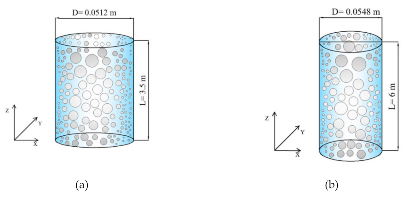
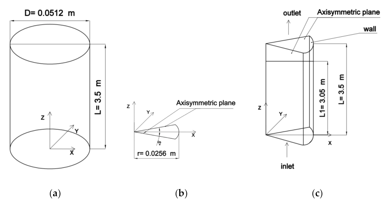
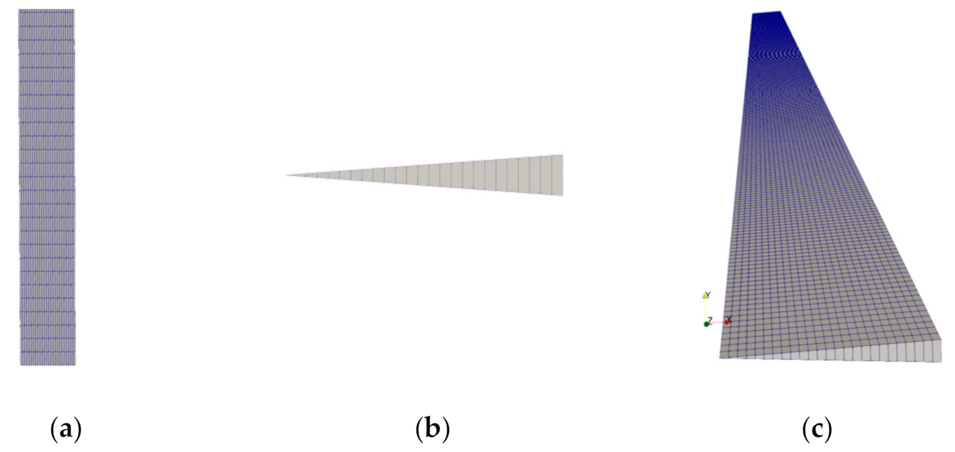
3.2. Computational Domain and Grid Independence Test

The first test case (Test 1) simulated in this paper was a circular bubble column studied by Lucas et al. [51]. The second test case (Test 2) was a circular bubble column studied by Banowski et al. [52]. Both test cases used the circular bubble columns with different diameters and heights. The column was filled with water (i.e., continuous liquid phase) at room temperature and atmospheric pressure, while water and gas flow was fed from the bottom of the column along the Z-axis. A sketch of the setup is shown in Figure 1.

According to the computing domain shown in Figure 1a, four sets of structural grids were selected and generated by ICEMCFD, which are All-grid-1, All-grid-2, All-grid-3, and All-grid-4, as listed in

Table 3. Grid schemes of the total flow field computing domain.

Grid Name	All-Grid-1	All-Grid-2	All-Grid-3	All-Grid-4
Number of mesh nodes along the flow direction	40	105	360	450
Number of section grids	1548	1548	2052	2052
Total number of grids	61,920	162,540	738,720	923,400

.

The different grid partitioning schemes are shown in Figure 2. The number of grids for All-grid-3 and All-grid-4 was increased along the flow direction and the cross-section. The aspect ratio of the grid was optimized by increasing the number of grids in the flow direction. The E-E two-fluid model was used to calculate the gas phase velocity of Test Case 1 in four schemes, and the appropriate number of grids was selected by comparison with the experimental data.

Boundary Condition Setting

Test 1 conditions: the apparent velocity of the gas phase was Ug = 0.0096 m/s, the water flow velocity was U_L = 1.0167 m/s, and the gas volume fraction was α_G = 1%. The inlet velocity of the gas phase can be calculated from the apparent velocity of the gas phase by using the following expression:

$$V_{inlet}=\frac{V_{super}\cdot OutletArea}{InletArea\cdot {\alpha }_{Inlet}}$$

(13)

where V_super is the apparent velocity of the gas phase, 0.0096 m/s, and the gas volume fraction at the inlet is α_G = 1%, thus the inlet velocity of the gas phase is V_inlet = 0.96 m/s. Other parameters are listed in

Table 4. Boundary condition parameters in OpenFoam.

Variable	Value of Inlet	Property of Inlet	Value of Outlet	Property of Outlet
Gas phase volume fraction $\mathsf{\alpha }$G	0.01	Fixed Value	zeroGradient	Zero Gradient
Liquid volume fraction 1-$\mathsf{\alpha }$G	0.99	Fixed Value	zeroGradient	Zero Gradient
Gas phase velocity ${\mathrm{U}}_{\mathrm{d}}$(m/s)	0.96	Fixed Value	$internalField	No slip
Liquid phase velocity ${\mathrm{U}}_{\mathrm{c}}$(m/s)	1.0167	Fixed Value	$internalField	No slip
Pressure $\mathrm{P}$ (pa)	101,325	Zero Gradient	$internalField	Fixed Value
Liquid turbulent kinetic energy $\mathrm{k}$	0.0041	Fixed Value	$internalField	Standard wall function
Kinetic energy dissipation rate of liquid phase turbulence $\mathsf{\epsilon }$	0.188	Fixed Value	$internalField	Standard wall function

.

The calculated gas velocities at different partitioning schemes are shown in Figure 3. Due to the increase in the number of grids along the cross-section and the flow directions, the calculated values of the gas phase velocity in the central region of the column in the schemes of All-grid-3 and All-grid-4 conformed to the experimental values, and more wall velocity values were obtained. The velocity of the gas phase near the column wall should approach 0, but the experimental data were incomplete due to the limitation of conditions. All-grid-3 and All-grid-4 were the partitioning schemes that can meet the requirements of this study. On the premise of satisfying the calculation accuracy requirements and shortening the calculation time, the partitioning scheme of All-grid-3 was the best one, shown as the red solid line in Figure 3.

The compute domain is shown in Figure 4, which the full flow field is shown in Figure 4a. The calculated flow field was considered as steady and the calculation domain as axisymmetric. To further save the calculation resources, a wedge was taken as the computational domain, which was extended along the Z-axis from a sector cut from the flow field with an angle of 5° and a radius of r = 0.0256 m. In other words, only 1/72 of the total flow field was calculated, as shown in Figure 4b,c.

The wedge grids in the following test cases were generated by the BlockMesh according to the All-grid-3 partitioning scheme, as shown in Figure 5, Axial mesh, as shown in Figure 5a, Section mesh is Figure 5b, Wedge 3D mesh is Figure 5c. In the process of calculating the wedge area with OpenFoam, the axisymmetric plane was set as the Wedge. The fully orthogonal grids with 28 (width) × 360 (height) were generated.

The calculation results of the Wedge-grid and All-grid-3 are shown in Figure 6. It can be seen that the partitioning scheme of the wedge grid can meet the calculation requirements.

3.3. Comparison of Different Drag Models

The drag force is the most important force among the inter-phase momentum forces. It defines the maximum velocity of a bubble in a continuous fluid driven by buoyancy [36]. The drag force mainly depends on the bubble shape, the relative velocity between dispersed and continuous phases, and the viscosity. Based on Test 1, different drag models were used to calculate the gas velocity. The SchiillerNaumann model [48] and Tomiyama model [49,50] were compared in this section, as shown in Figure 7. The gas velocity calculated by the former is significantly higher than latter and much higher than the experimental value, as the blue dotted line shown in Figure 7. The gas phase velocity calculated by the Tomiyama mode is in good agreement with the experimental results, as the red solid line shown in Figure 7.

Due to the application of E_O in the Tomiyama model, the increase in resistance in the flow field caused by bubble deformation and the decrease in gas phase velocity was taken into account, while it was not in the Schiiller–Naumann model.

4. Results and Discussion

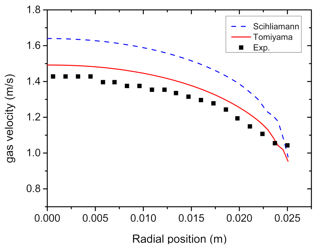
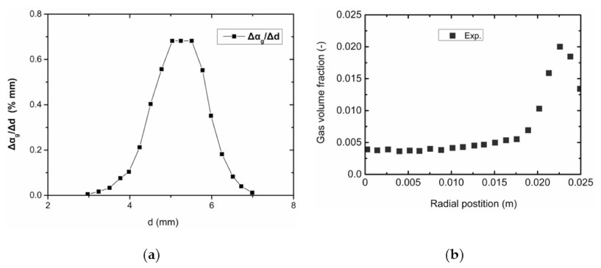
4.1. Experimental Verification Case 1 (Unimodal Distribution)

The experimental data were obtained from the literature [51]. The experiment was conducted on the MTLOOP device. The experimental data of the gas volume fraction were captured by a metal grid sensor equipped with an electrode, which has been widely used in the study of the flow pattern of gas–liquid bubble flow and of the distribution of gas volume fraction in vertical pipes.

In the experimental device for the gas-liquid two-phase flow, the diameter of the pipe in the experimental section was D = 0.0512 m and the height was L = 3.5 m. The test section was located at L/D = 59.6, that is, the distance from the entrance section was L1 = 3.05 m, as shown in Figure 4. The experimental data are shown in Figure 8.

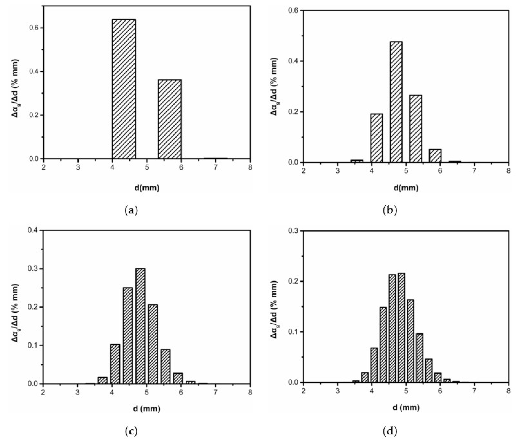
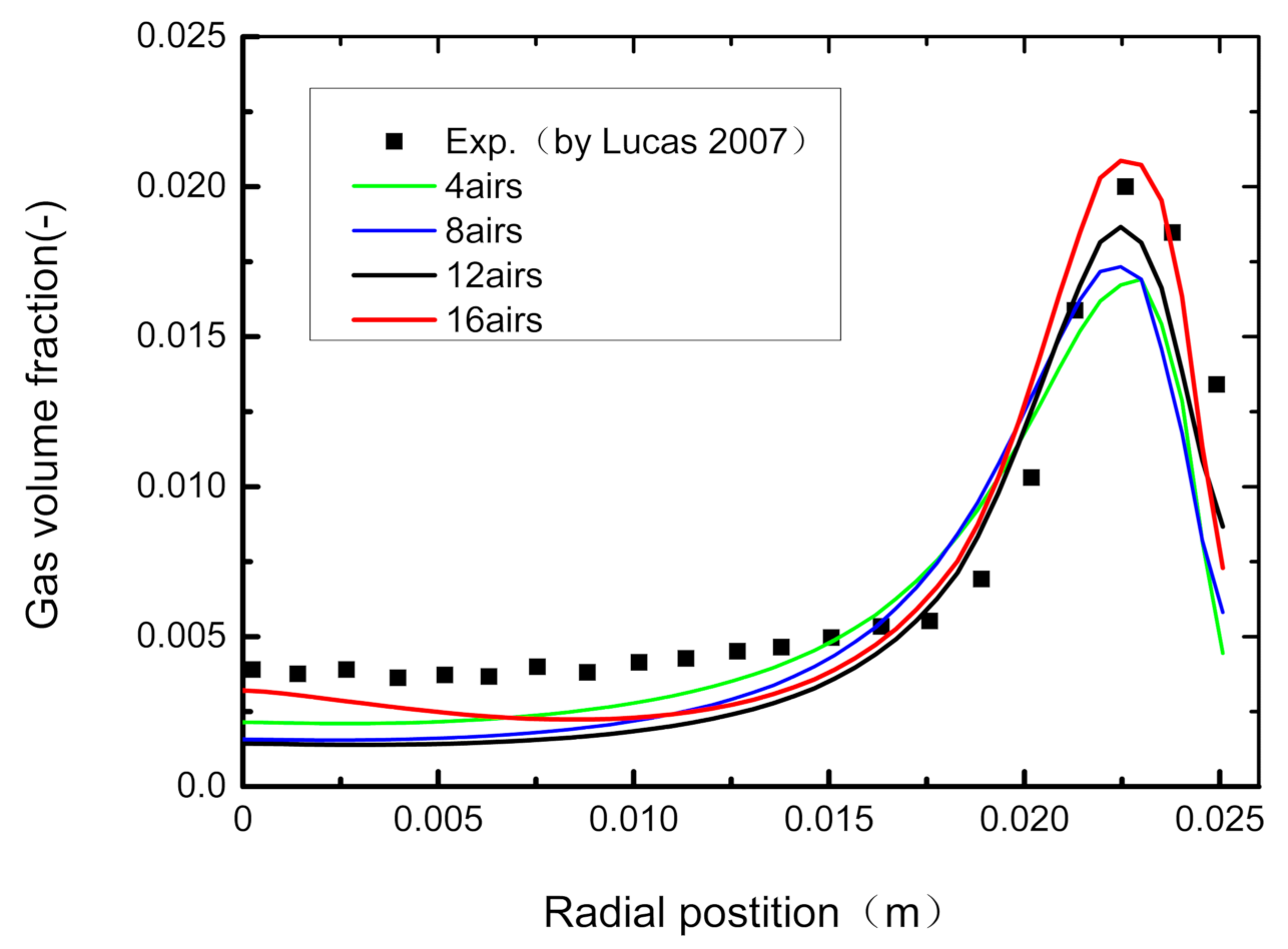
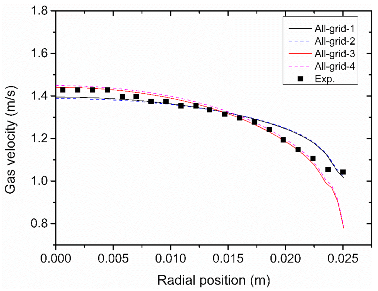
4.1.1. Influence of Group Number of the Dispersed Phase on the Calculation Results

In order to calculate the distribution of gas volume fraction of the bubble flow in pipes using the multi-fluid model, it is necessary to determine the bubble diameter distribution. The commonly used distribution function is the normal distribution. Some scholars believe that the bubble distribution in the gas-liquid two-phase flow in a pipe is more inclined to be lognormal distribution [53]. In this section, the bubble diameter distribution is reconstructed by using the lognormal distribution function according to the average bubble diameter and the gas volume fraction provided in the experiment, as well as the gas volume fraction along the radius of the tested pipe section.

To obtain accurate details of the flow field of the polydisperse bubble flow, the more groups of the dispersed phase, the closer it is to the real flow field. But the number of groups is restricted by the actual test conditions in the laboratory. Therefore, it is necessary to determine an appropriate grouping scheme, where bubbles with both small and large diameters should exist, and the gas volume fraction of each diameter shall conform to the correct probability distribution function.

The distribution of bubbles along the radius of the pipe can be roughly divided into three regions. When the bubble diameter dB is greater than 5.8 mm, the lift force changes direction and points to the pipe center, pushing the bubble toward the center; when 0.4 < dB < 5 mm, bubbles will move toward the pipe wall forming a peak of gas volume fraction on the wall; when 5 < dB < 5.8 mm, the bubble movement is affected by turbulence and bubble response, forming an intermediate transition region. According to the test data (see Figure 8a), the bubble diameters vary from 3 mm to 7 mm, so the grouping scheme of four was used. In this paper, bubbles with different diameters were divided into 4 groups, 8 groups, 12 groups, and 16 groups, hereinafter referred to as 4 airs, 8 airs, 12 airs, and 16 airs. The multi-fluid model is used to calculate the distribution of gas volume fraction along the pipe radius in each scheme. The calculation results were compared with experimental data (see Figure 8b for black rectangular blocks) to analyze the influence of group numbers on the calculated values. Although the gas volume fraction of each group varies with the bubble diameter distribution, the average diameter of the bubbles in each group is 4.8 mm, the total gas volume fraction is 0.01, and the bubble injection speed is 0.96 m/s. The bubble diameter distributions are shown in Figure 9a–d, and the calculated results are shown in Figure 10.

When the bubbles are grouped into four, and the bubble diameters are divided at the same interval from 3 mm to 7 mm, there is a small component with the bubble diameter of dB > 5.8 mm in the dispersed phase, as shown in Figure 9a. Although the calculated values of the gas volume fraction are consistent with the experimental values (see Figure 8b for black rectangular blocks) in the wall area (0.02 < r < 0.025 m), they are still lower than the experimental values in the central area (0 < r < 0.015 m). The reason is that in this scheme, the proportion of large bubbles of dB > 5.8 mm is lower, and the proportion of large bubbles with different diameters in the total gas volume fraction is small, as the green solid line shown in Figure 10.

When the bubbles are grouped into eight, the proportion of bubbles of dB > 5.8 mm increases, so the calculated value is closer to the experimental value in the central area (0 < r < 0.015 m), as the blue solid line shown in Figure 10. It is worth noting that the calculated value in the wall area is quite different from the experimental value due to the neglecting of the small diameter bubbles in the grouping scheme. Therefore, the number of bubble groups is an important factor affecting the experimental results. To obtain a more accurate calculation result along the pipe radius, the equal interval grouping schemes of 12 airs and 16 airs are simulated. With the increasing of groups, the calculated values gradually approach the experimental value at the pipe wall, and the deviation becomes smaller in the central area, as the 12 airs (black solid line) and 16 airs (red solid line) shown in Figure 10.

It is obvious that the results of the 16 airs (red solid line in Figure 10) are closer to the experimental values than others both in the wall area and the central area. As the number of groups decreases from 16 airs to 4 airs, the distribution of gas volume fraction also decreases due to the weakening of the multi-dispersion characteristic of the gas–liquid two-phase flow field in this experimental case. Therefore, 16airs of bubble diameters are proposed in this paper as the scheme of grouping.

In fact, according to the analysis of the test data, as shown in Figure 8a, if dividing the bubbles with the interval of ∆dB = 0.25 mm in the range from 3 mm to 7 mm [51], the number of bubble groups is 16. This indicates that the bubble diameter interval has a significant impact on the measuring accuracy of the gas volume fraction during the experiment. At the same time, the accuracy of the multi-fluid model in calculating the gas volume fraction of the polydisperse gas–liquid two-phase flow is verified.

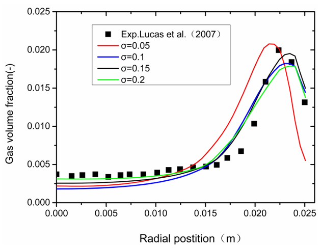
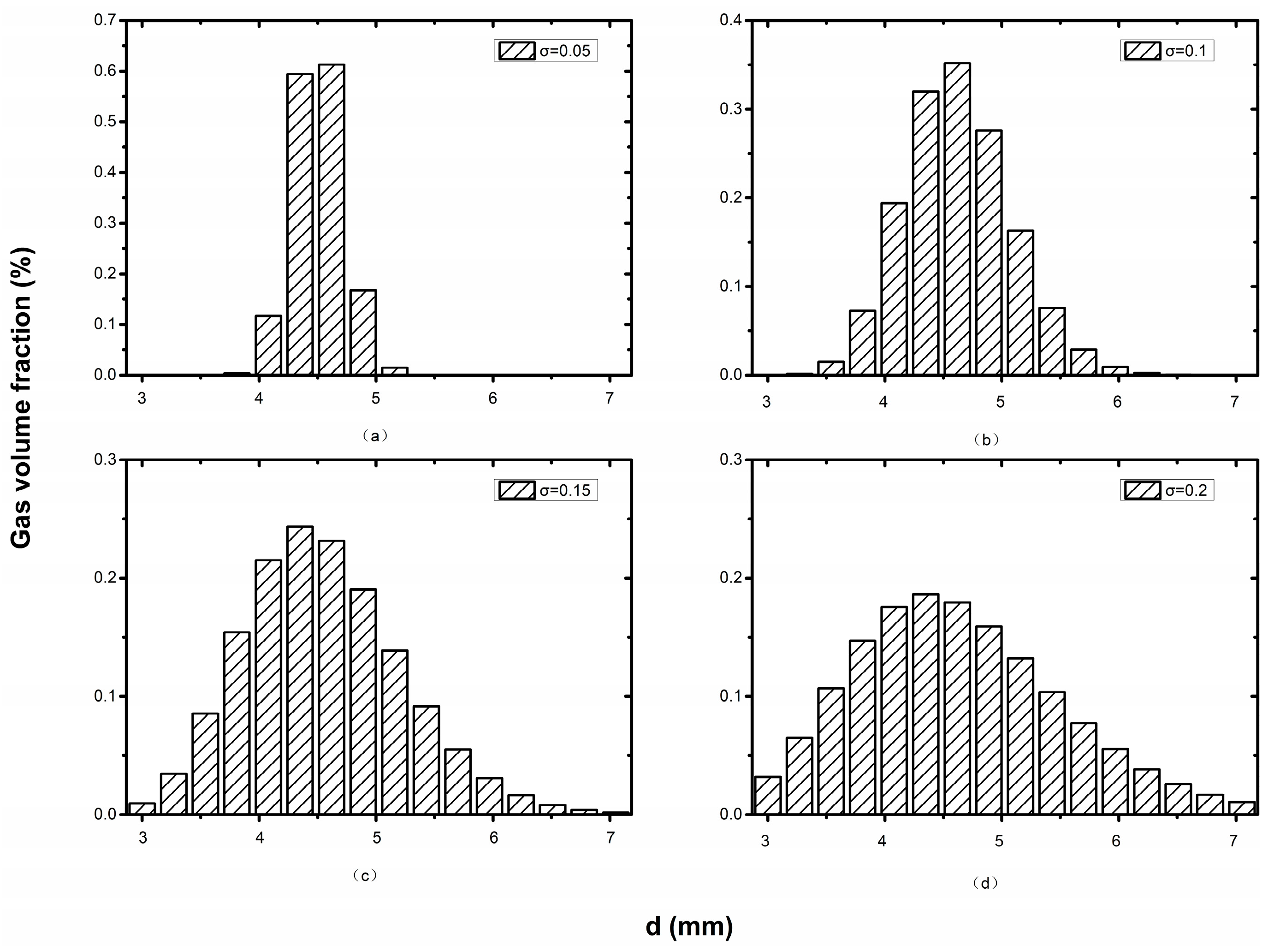
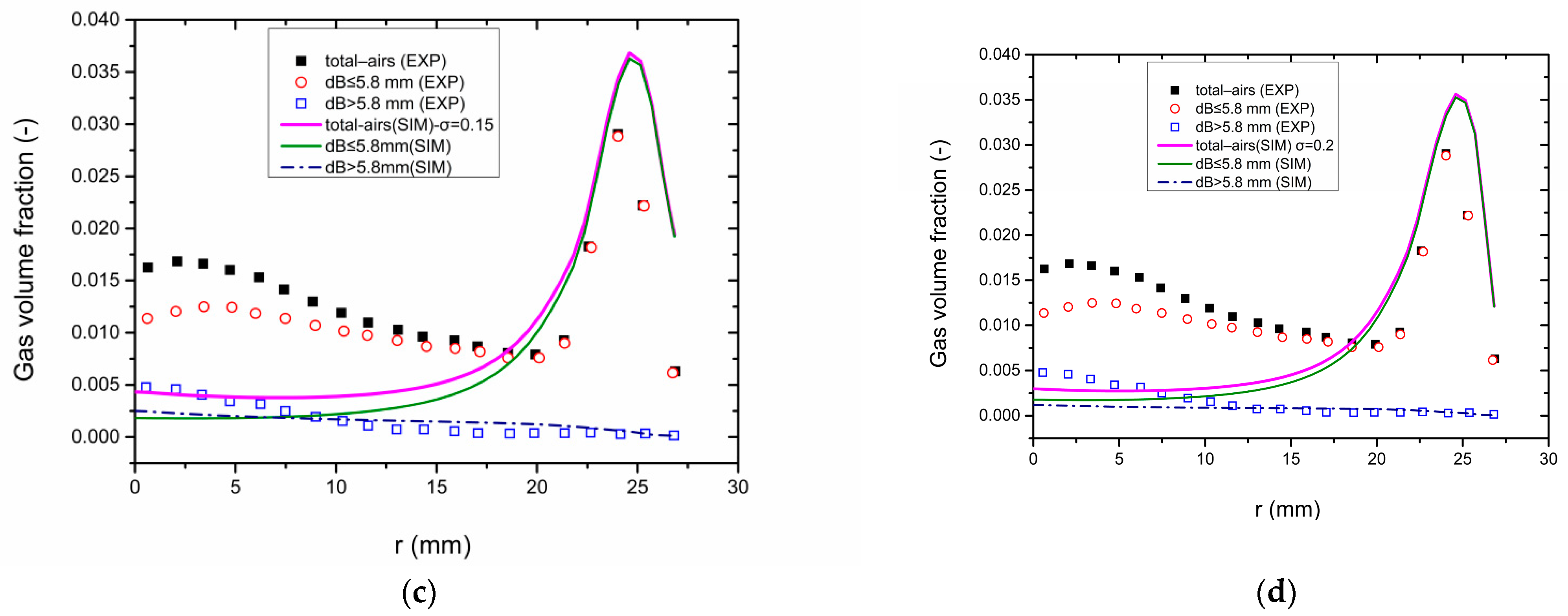
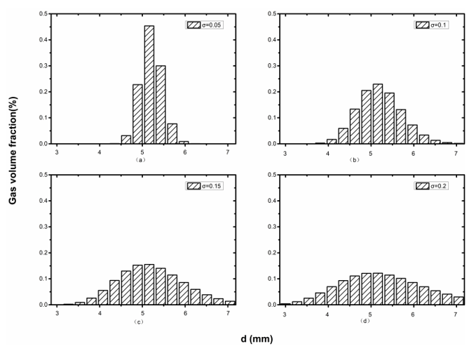
4.1.2. Influence of Parameter σ on the Calculation Results

The average diameter and total gas volume fraction can be calculated from the test data (Figure 8a) by a lognormal distribution. The histogram of bubble diameter distribution with different standard deviations is shown in Figure 11.

The standard deviation of Figure 11a is 0.05. It can be seen that the bubbles with a diameter of 5.1 mm have the largest proportion, 0.42%; while those smaller than 4.5 mm or larger than 6 mm have a small proportion. By comparing the calculated results (the red solid line in Figure 12) with the experimental data (the black rectangular blocks in Figure 8b), it can be seen that the calculated gas volume fractions at the wall area are higher than the experimental value, while those at the central area are lower. The reason is that when σ = 0.05, the proportion of bubbles smaller than 5.8 mm is lower than the experimental value, which leads to a high proportion of bubbles smaller than 5.8 mm in the flow field.

The standard deviation of Figure 11b is 0.1. Although bubbles with a diameter of 5.1 mm accounted for the highest proportion, which is 0.24%, the proportion of bubbles larger than 5.8 mm is increased. Therefore, the gas volume fraction calculated by the multi-fluid model is consistent with the experimental value in the central area, as the blue solid line shown in Figure 12, but it is still lower in the wall area.

The standard deviation of Figure 11c is 0.15. The bubble diameter distribution range is further expanded, that is, the proportions of bubbles smaller than 4.5 mm and larger than 6 mm are greatly increased, and the polydisperse phase characteristics of the bubble flow are significant, leading to the higher calculated gas volume fraction higher in the central area and lower in the wall area when compared with the experimental value, as the black solid line shown in Figure 12.

The standard deviation of Figure 11d is 0.2. The bubble diameter distribution range completely covers the range of 3 mm to 7 mm, and there is little difference between bubbles of different diameters. The polydisperse phase characteristics are more significant, leading to the calculated gas volume fraction higher in the central area and slightly lower in the wall area when compared with the experimental value, as the green solid line shown in Figure 12. The comparison shows that with the increasing of the standard deviation, the multi-dispersion characteristics of the bubble flow gradually manifest, which has a significant impact on the distribution of gas volume fraction calculated by the multi-fluid model, leading to its increasing in the central area from lower to higher than the experimental value.

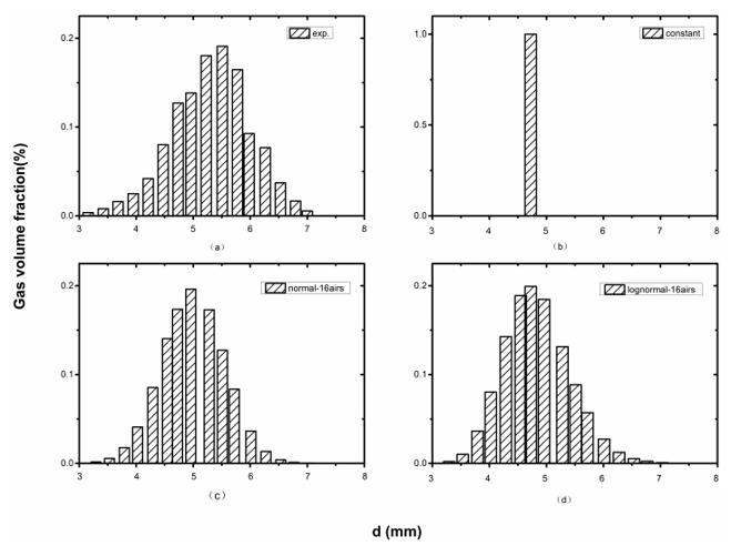
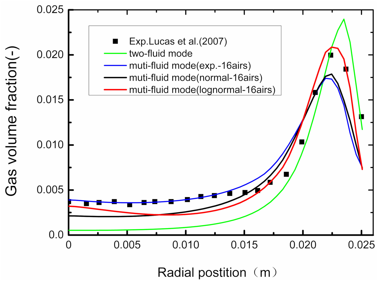
4.1.3. Influence of Different Distribution Functions on the Calculation Results

The bubbles are divided into 16 groups with an interval of 0.25 mm from 3 mm to 7 mm. The distribution of gas volume fraction of bubbles with different diameters, which is calculated according to the histogram of bubble diameter distribution (Figure 8a), is shown in Figure 13a. The average bubble diameter is 4.8 mm, as shown in Figure 13b. The histogram of the distribution of the gas volume fraction fitted with the normal distribution function with σ = 0.55 is shown in Figure 13c. The histogram fitted with the lognormal distribution function with σ = 0.11 is shown in Figure 13d.

Figure 13a shows the histogram of bubble diameter distribution obtained from the experiment when $\overline{\mathrm{d}}$ = 4.8 mm and α_G = 1%. The distribution of gas volume fraction along the pipe radius calculated by the multi-fluid model is the blue solid line in Figure 14. Although the calculated gas volume fraction in the wall area is lower than the experimental value, the calculated value in the central area agrees with the experimental value. This indicates that the distribution of bubble diameter affects the distribution of gas volume fraction along the radius in the multi-phase bubble flow.

It is assumed that the bubble flow measured in this experiment is monodisperse. According to the properties of monodisperse bubble flow, the diameter of each bubble in the flow field is treated as the same, d = 4.8 mm and α_G = 1%. The histogram of bubble diameter distribution is reconstructed with the uniform distribution function, as shown in Figure 13b, and the E-E two-fluid model is used to calculate the distribution of gas volume fraction. When using the average bubble diameter to represent the bubble diameter distribution of the entire flow field, the distribution of gas volume fraction along the pipe radius calculated by the two-fluid model is the green solid line shown in Figure 14. There is a peak value near the pipe wall, slightly higher than the experimental value [51], as the black rectangular blocks that are shown in Figure 8b. However, the calculated values are significantly lower than the experimental values in the central area. This is caused by the treating of the flow field as the single dispersed bubble flow, the using of average diameter as the diameter of bubbles in the polydisperse system, and the neglecting of the multi-dispersion characteristics of bubbles with different diameters.

The bubble diameter distribution in the flow field is reconstructed by the normal distribution function, as shown in Figure 13c. The distribution of gas volume fraction along the pipe radius is calculated by the multi-fluid model, as the black solid line shown in Figure 14. The black solid line and the blue solid line are similar, slightly lower than the experimental value at the wall area, and consistent in the central area. This indicates that the proportion of bubbles smaller than 5.8 mm is low.

The distribution of bubble diameters in the flow field is reconstructed by the lognormal distribution function, as shown in Figure 13d. The distribution of gas volume fraction along the pipe radius is calculated by using the multi-fluid model, as the red solid line shown in Figure 14. The calculated value is consistent with the experimental value (black rectangular blocks in Figure 14) both in the wall area and the central area. It is shown that the bubble diameter distribution function is more consistent with the lognormal distribution if the average bubble diameter and the gas volume fraction are the same in the polydisperse bubble flow.

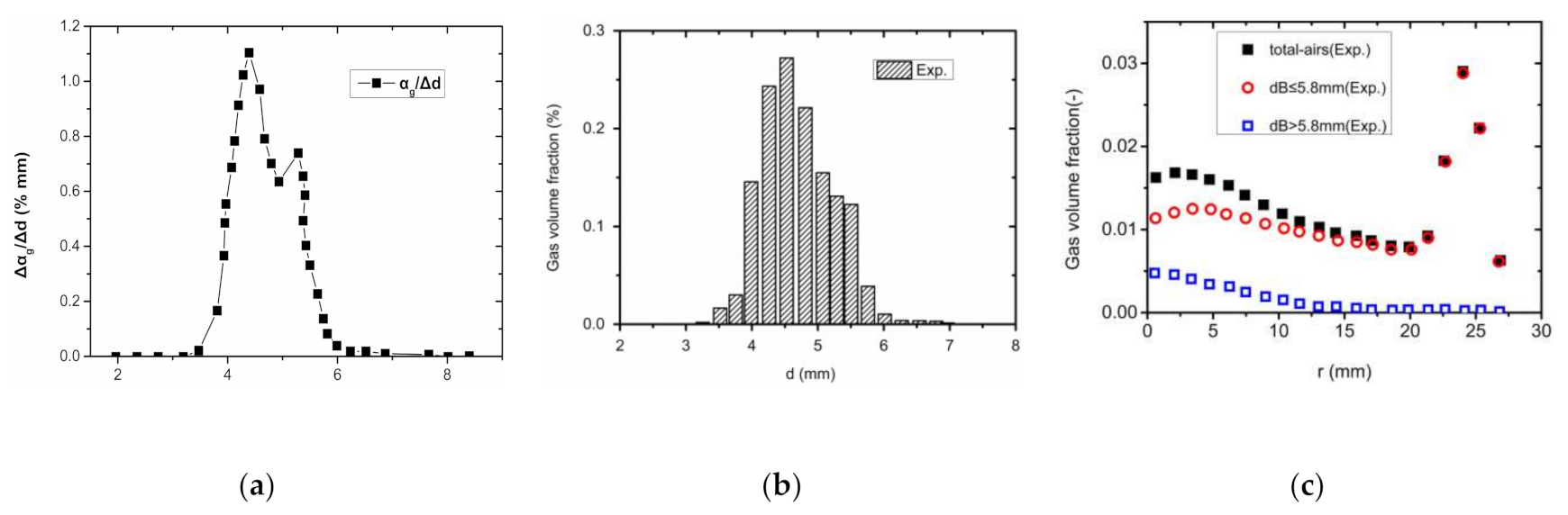
4.2. Experimental Verification Case 2 (Bimodal Distribution)

To further verify the accuracy and adaptability of the multi-fluid model in calculating the gas volume fraction in the polydisperse gas-liquid two-phase flow, a second example [52] is introduced. Compared with case 1, the apparent velocity of bubbles in case 2 was increased to U_G = 0.0151 m/s. The diameter of the pipe used was D = 54.8 mm, the length of the pipe was L = 6 m, the test section was located at L/D = 59.7, that is, L = 3.27 m, the gas injection rate was 1.51 m/s, the total gas volume fraction of bubbles in the pipe was α_G = 0.01, and the liquid flow velocity was U_L = 1.017 m/s. In case 2, the proportion of large bubbles increases significantly with the increase in the bubble apparent velocity, and the bubble diameter distribution presents a bimodal characteristic, as shown in Figure 15a. Figure 15b is a histogram of bubble diameter distribution calculated according to Figure 15a. The flow field is mainly occupied by bubbles with diameters of 4.5 mm and 5.6 mm. The test results show that there is one peak value at the pipe center and another one on the pipe wall. The distribution of gas volume fraction has a bimodal characteristic along the radius. Bubbles with dB ≤ 5.8 mm are converged at the wall area, while bubbles with dB > 5.8 mm are converged at the central area, as shown in Figure 15c.

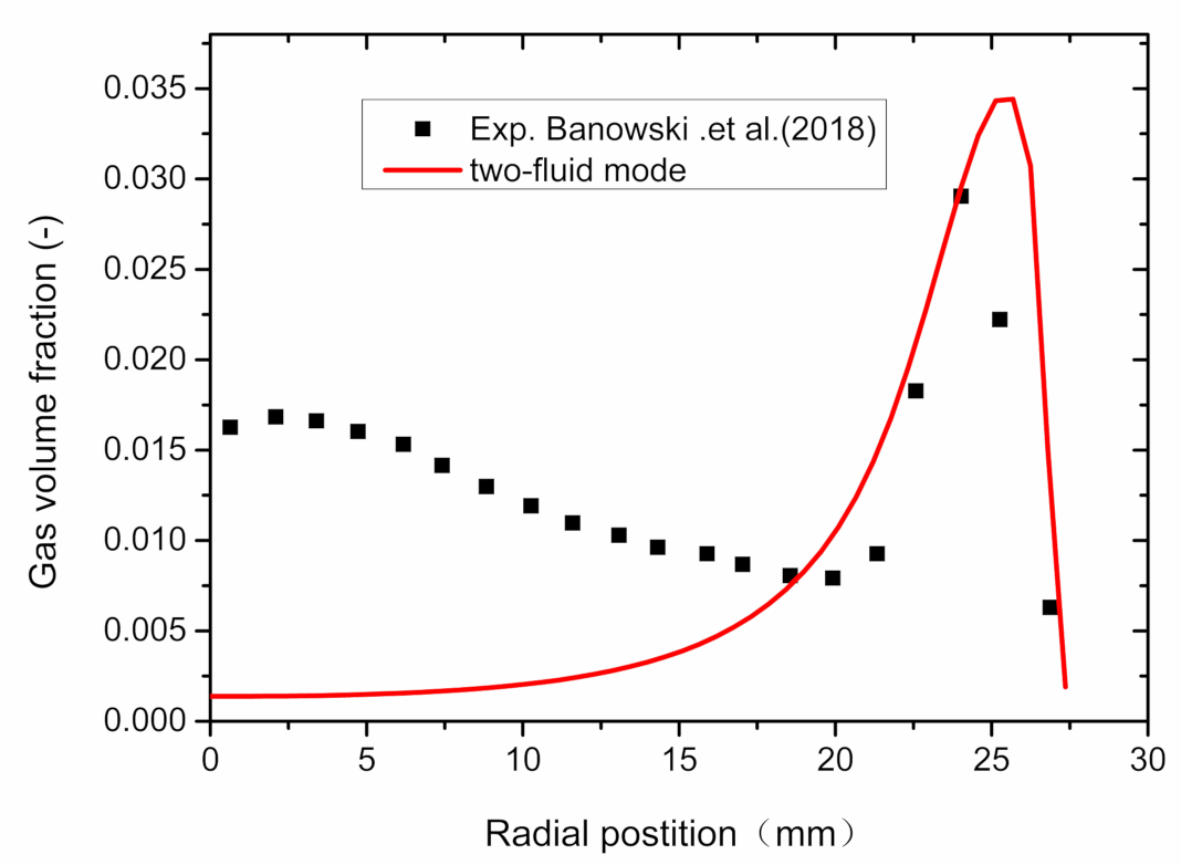
4.2.1. Calculation Results of E-E Two-Fluid Model

To compare the advantages and disadvantages of the multi-fluid model and the two-fluid model in simulating the polydisperse phase flow field, the average bubble diameter can be calculated as 4.8 mm according to the test results in Figure 15b, and the calculation results using the two-fluid model are shown in Figure 16. Most of the bubbles are converged near the wall leading to a peak value slightly higher than the experimental value, while the gas volume fraction in the center is close to zero, which is far away from the experimental value. The results show that the two-fluid model cannot be used to accurately predict the distribution of the gas volume fraction along the radius in the polydisperse bubble flow.

The reason is that there is only one single average bubble diameter when using the two-fluid model., which in this case is 4.8 mm. However, the calculated results show that bubbles smaller than 5.8 mm are converged in the wall area presenting an obvious unimodal distribution, as the red solid line shown in Figure 16; while those larger than 5.8 mm have not been calculated, resulting in a large deviation with the experimental value in the central area. Erasing the characteristics of the polydisperse flow field has limited the use of the two-fluid model in calculating the bubble flow with the polydisperse phase, which can also be seen in Table 2.

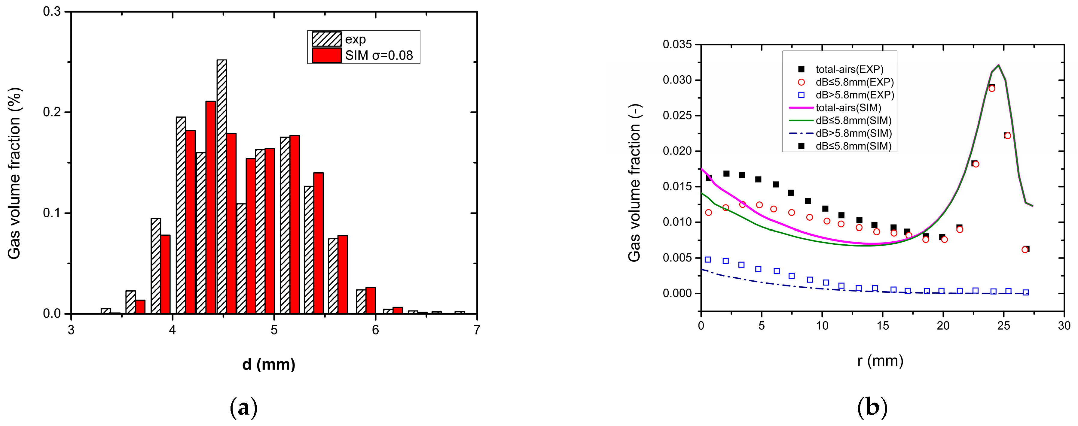
4.2.2. Calculation Results of Multi-Fluid Model with Unimodal and Bimodal Lognormal Distribution of Bubbles Diameters

The bubble diameter distribution is reconstructed into 16 groups with different diameters and fitted with the unimodal lognormal distribution. The unimodal distribution functions with different standard deviations (σ = 0.05, 0.1, 0.15, and 0.2) are fitted, as shown in Figure 17. The corresponding calculation results are shown in Figure 18a–d. The proportion of large bubble phase in the central area fitted by the unimodal lognormal distribution is far lower than the experimental value, as the blue dotted line shown in Figure 18a. The results show that the gas volume fraction of the bubbles larger than 5.8 mm is almost zero, while the bubbles smaller than 5.8 mm are concentrated. The calculated value of the total gas volume fraction in the flow field (purple solid line) and that of bubbles less than 5.8 mm (green solid line) coincide together, forming a peak on the pipe wall, and this calculation result corresponds to the histogram of bubble diameter distribution in Figure 17a. The results show that the gas volume fraction at the wall area is basically consistent with the experimental data, but there is an obvious deviation in the central area ((r = 0 m to r = 0.018 m). This indicates that the distribution of bubbles with different diameters fitted by the unimodal lognormal distribution function does not fit the actual distribution pattern in this case.

The bubble distribution of case 2 cannot be described by using the unimodal lognormal distribution, which is also proved by the corresponding results of other different standard deviations in Figure 17b–d and Figure 18b–d.

According to the experimental data (Figure 15b), the bimodal lognormal distribution function is used to reconstruct the bubble diameter distribution, as shown in Figure 19. In accordance with the distribution (the red rectangle bar in Figure 19a), the multi-fluid model is used to calculate the distribution of gas volume fraction along the pipe radius. The calculation results are shown in Figure 19b.

The results show that the calculated values of bubbles with different diameters along the radius are in agreement with the experimental values. Case 2 has a higher gas volume fraction than case 1, and the bubble diameter distribution is consistent with the bimodal lognormal distribution.

5. Conclusions

The two-fluid model and the multi-fluid model were used to simulate the upward bubble flows. The simulation results were compared with the experimental data as reported in the published literature. Based on the verification, it is concluded that:

(1) The E-E multi-fluid model can accurately predict the distribution of gas volume fraction along the pipe radius in both the polydisperse bubble flow and the monodisperse flow. For small superficial gas velocity, it shows a monodisperse flow pattern. Both the two-fluid model and the multi-fluid model can be used to obtain the unimodal distribution of the gas volume fraction along the pipe radius, while the calculated results of the multi-fluid model are more consistent with the experimental data.

(2) When the superficial gas velocity increases to U_G = 0.0151 m/s and the flow velocity is U_L = 1.0167 m/s, more large bubbles (d_B > 5.8 mm) will appear. The bubble diameter distribution is bimodal, and the distribution of the gas volume fraction is also bimodal along the pipe radius. In this case, the multi-fluid model can accurately predict the distribution trend, while there will be a large error if using the two-fluid model.

(3) The distribution function of bubble diameters in the polydisperse bubble flow field is studied and it is verified that the diameter distribution of bubble flow in a pipe conforms to the lognormal distribution, and the parameters of different distribution functions have a significant influence on the calculation results.

References

1. Delhaye, J.M. Basic Equations for Two-Phase Flow Modeling. In Two-Phase Flow, and Heat Transfer in the Power and Process Industries; Hemisphere: New York, NY, USA, 1981. [Google Scholar]
2. Bankoff, S.G. Handbook of Multiphase Systems. Am. Sci. 1983, 71. Available online: https://www.jstor.org/stable/i27851891 (accessed on 5 September 2021).
3. Krepper, E.; Lucas, D.; Prasser, H. On the modelling of bubbly flow in vertical pipes. Nucl. Eng. Des. 2005, 235, 597–611. [Google Scholar] [CrossRef]
4. Colombo, M.; Fairweather, M. Accuracy of Eulerian–Eulerian, two-fluid CFD boiling models of subcooled boiling flows. Int. J. Heat Mass Transfer 2016, 103, 28–44. [Google Scholar] [CrossRef]
5. Panicker, N.; Passalacqua, A.; Fox, R.O. On the hyperbolicity of the twofluid model for gas–liquid bubbly flows. Appl. Math. Model. 2018, 57, 432–447. [Google Scholar] [CrossRef] [Green Version]
6. Legendre, D.; Magnaudet, J. A note on the lift force on a spherical bubble or drop in a low-Reynolds-number shear flow. Phys. Fluids 1997, 9, 3572. [Google Scholar] [CrossRef] [Green Version]
7. Legendre, D.; Magnaudet, J. The lift-force on a spherical bubble in a viscous linear shear flow. J. Fluid Mech. 1998, 368, 81. [Google Scholar] [CrossRef]
8. Hibiki, T.; Ishii, M. Lift force in bubbly flow systems. Chem. Eng. Sci. 2007, 62, 6457–6474. [Google Scholar] [CrossRef]
9. Rzehak, R.; Krepper, E.; Lifante, C. Comparative study of wall-force models for the simulation of bubbly flows. Nucl. Eng. Des. 2012, 253, 41–49. [Google Scholar] [CrossRef]
10. Lopez de Bertodano, M.; Lahey, R.T.; Jones, O.C. Phase distribution in bubbly two-phase flow in vertical ducts. Int. J. Multiph. Flow 1994, 20, 805–818. [Google Scholar] [CrossRef]
11. Kataoka, I.; Serizawa, A.; Besnard, D.C. Prediction of turbulence suppression and turbulence modeling in bubbly two-phase flow. Nucl. Eng. Des. 1993, 141, 145–158. [Google Scholar] [CrossRef]
12. Sato, Y.; Sekoguchi, K. Liquid velocity distribution in two-phase bubbly flow. Int. J. Multiph. Flow 1975, 2, 79–95. [Google Scholar] [CrossRef]
13. Tomiyama, A.; Matsuoka, T.; Fukuda, T.; Sakaguchi, T. A Simple Numerical Method for Solving an Incompressible Two-Fluid Model in a General Curvilinear Coordinate System, Advances in Multiphase Flow; Elsevier: Amsterdam, The Netherlands, 1995; Volume 241. [Google Scholar]
14. Tomiyama, A.; Shimada, N. A Numerical Method for Bubbly Flow Simulation based on a Multi-Fluid Model. ASME J. Press. Vessel Technol. 2001, 123, 510. [Google Scholar] [CrossRef]
15. Tomiyama, A. Modeling and hybrid simulation of bubbly flow. Multiph. Sci. Technol. 2005, 17, 445–482. [Google Scholar] [CrossRef]
16. Laın, S.; Bröder, D.; Sommerfeld, M.; Göz, M.F. Modelling hydrodynamics and turbulence in a bubble column using the Euler-Lagrange procedure. Int. J. Multiph. Flow 2002, 28, 1381–1407. [Google Scholar] [CrossRef]
17. McGraw, R. Description of aerosol dynamics by the quadrature method of moments. Aerosol. Sci. Tech. 1997, 27, 255–265. [Google Scholar] [CrossRef]
18. Dorao, C.A.; Jakobsen, H.A. A least squares method for the solution of population balance problems. Comput. Chem. Eng. 2006, 30, 535–547. [Google Scholar] [CrossRef]
19. Petitti, M.; Vanni, M.; Marchisio, D.L.; Buffo, A.; Podenzani, F. Simulation of coalescence, break-up and mass transfer in a gas–liquid stirred tank with CQMOM. Chem. Eng. J. 2013, 228, 1182–1194. [Google Scholar] [CrossRef]
20. Lo, S. Application of the MUSIG model to bubbly flows AEAT-1096. AEA Technol. 1996, 230, 8216–8246. [Google Scholar]
21. Krepper, E.; Lucas, D.; Frank, T.; Prasser, H.; Zwart, P. The inhomogeneous MUSIG model for the simulation of polydispersed flows. Nucl. Eng. Des. 2008, 238, 1690–1702. [Google Scholar] [CrossRef]
22. Lucas, D.; Rzehak, R.; Krepper, E.; Ziegenhein, T.; Liao, Y.; Kriebitzsch, S.; Apanasevich, P. A strategy for the qualification of multi-fluid approaches for nuclear reactor safety. Nucl. Eng. Des. 2016, 299, 2–11. [Google Scholar] [CrossRef]
23. Xiao, Q.; Wang, J.; Yang, N.; Li, J. Simulation of the multiphase flow in bubble columns with stability-constrained multi-fluid CFD models. Chem. Eng. J. 2017, 329, 88–99. [Google Scholar] [CrossRef]
24. Li, D.; Li, Z.; Gao, Z. Compressibility induced bubble size variation in bubble column reactors: Simulations by the CFD-PBE. Chin. J. Chem. Eng. 2018, 26, 13–17. [Google Scholar] [CrossRef]
25. Li, D.; Buffo, A.; Podgórska, W.; Marchisio, D.L.; Gao, Z. Investigation of droplet breakup in liquid–liquid dispersions by CFD–PBM simulations: The influence of the surfactant type. Chin. J. Chem. Eng. 2017, 25, 1369–1380. [Google Scholar] [CrossRef]
26. Zhang, X.B.; Zheng, R.Q.; Luo, Z.H. CFD-PBM Simulation of Bubble Columns: Effect of Parameters in the Class Method for Solving PBEs. Chem. Eng. Sci. 2020, 226, 115853. [Google Scholar] [CrossRef]
27. An, M.; Guan, X.; Yang, N. Modeling the Effects of Solid Particles in CFD-PBM Simulation of Slurry Bubble Columns. Chem. Eng. Sci. 2020, 223, 115743. [Google Scholar] [CrossRef]
28. Li, D.; Marchisio, D.; Hasse, C.; Lucas, D. Comparison of Eulerian QBMM and classical Eulerian–Eulerian method for the simulation of polydisperse bubbly flows. AIChE J. 2019, 65, e16732. [Google Scholar] [CrossRef]
29. Li, D.; Marchisio, D.; Hasse, C.; Lucas, D. twoWayGPBEFoam: An open-source Eulerian QBMM solver for monokinetic bubbly flows. Comput. Phys. Commun. 2019, 250, 107036. [Google Scholar] [CrossRef]
30. Ishii, M. Thermo-fluid dynamic theory of two-phase flow. NASA Sti/Recon Tech. Rep. A 1976, 75, 29657. [Google Scholar]
31. Drew, D.A. Continuum Modeling of Two-Phase Flows. In Theory of Dispersed Multiphase Flow; Academic Press: Cambridge, MA, USA, 1983; pp. 173–190. [Google Scholar]
32. Jackson, R. Locally averaged equations of motion for a mixture of identical spherical particles and a Newtonian fluid. Chem. Eng. Sci. 1997, 52, 2457–2469. [Google Scholar] [CrossRef]
33. Tomiyama, A.; Kataoka, I.; Zun, I.; Sakaguchi, T. Drag coe8cients of single bubbles under normal and micro gravity conditions. JSME Int. J. Ser. B 1998, 41, 472–479. [Google Scholar] [CrossRef]
34. Tomiyama, A.; Tamai, H.; Zun, I.; Hosokawa, S. Transverse migration of single bubbles in simple shear flows. Chem. Eng. Sci. 2002, 57, 1849–1858. [Google Scholar] [CrossRef]
35. Hosokawa, S.; Tomiyama, A.; Misaki, S.; Hamada, T. Lateral migration of single bubbles due to the presence of wall. In Proceedings of the ASME 2002 Joint US-European Fluids Engineering Division Conference, Montreal, QC, Canada, 14–18 June 2002; American Society of Mechanical Engineers: Montreal, QC, Canada, 2002. [Google Scholar]
36. Biesheuvel, A.; Gorissen, W.C.M. Void fraction disturbances in a uniform bubbly fluid. Int. J. Multiph. Flow 1990, 16, 211–231. [Google Scholar] [CrossRef] [Green Version]
37. Li, D.; Christian, H. Simulation of bubbly flows with special numerical treatments of the semi-conservative and fully conservative two-fluid model. Chem. Eng. Sci. 2017, 174, 25–39. [Google Scholar] [CrossRef]
38. Rusche, H. Computational Fluid Dynamics of Dispersed Two-Phase Flows at High Phase Fractions. Ph.D. Thesis, University of London, London, UK, 2003. [Google Scholar]
39. Sharma, S.L.; Hibiki, T.; Ishii, M.; Schlegel, J.P.; Buchanan, J.R., Jr.; Hogan, K.J.; Guilbert, P.W. An interfacial shear term evaluation study for adiabatic dispersed air–water two-phase flow with the twofluid model using CFD. Nucl. Eng. Des. 2017, 312, 389–398. [Google Scholar] [CrossRef]
40. Bhusare, V.H.; Dhiman, M.K.; Kalaga, D.V.; Roy, S.; Joshi, J.B. CFD simulations of a bubble column with and without internals by using OpenFOAM. Chem. Eng. J. 2017, 317, 157–174. [Google Scholar] [CrossRef]
41. Lahey, R.T., Jr. The simulation of multidimensional multiphase flows. Nucl. Eng. Des. 2005, 235, 1043–1060. [Google Scholar] [CrossRef]
42. Song, Q.; Luo, R.; Yang, X.Y.; Wang, Z. Phase distributions for upward laminar dilute bubbly flows with non-uniform bubble sizes in a vertical pipe. Int. J. Multiph. Flow 2001, 27, 379–390. [Google Scholar] [CrossRef]
43. Kashinsky, O.N.; Timkin, L. Slip velocity measurements in an upward bubbly flow by combined LDA and electrodiffusional techniques. Exp. Fluids 1999, 26, 305–314. [Google Scholar] [CrossRef]
44. Mohseni, K.; Shkoller, S.; Kosović, B.; Marsden, J.E. Numerical simulations of the lagrangian averaged navier-stokes (lans-α) equations for forced homogeneous isotropic turbulence. American institute of aeronautics & astronautics. Phys. Fluids 2003, 15, 524. [Google Scholar] [CrossRef]
45. Lahey, R.T.; Drew, D.A. The analysis of two-phase flow and heat transfer using a multidimensional, four field, two-fluid model. Nucl. Eng. Des. 2001, 204, 29–44. [Google Scholar] [CrossRef]
46. Ma, T.; Santarelli, C.; Ziegenhein, T.; Lucas, D.; Fröhlich, J. Direct numerical simulation–based Reynolds-averaged closure for bubble-induced turbulence. Phys. Rev. Fluids 2017, 2, 034301. [Google Scholar] [CrossRef]
47. Issa, R.I.; Gosman, A.D.; Watkins, A.P. The computation of compressible and incompressible recirculating flows by a non-iterative implicit scheme. J. Comput. Phys. 1986, 62, 66–82. [Google Scholar] [CrossRef]
48. Ishii, M.; Mishima, K. Two-fluid model and hydrodynamic constitutive relations. Nucl. Eng. Des. 1984, 82, 107–126. [Google Scholar] [CrossRef]
49. Ahmadi-Befrui, B.; Gosman, A.D.; Issa, R.I.; Watkins, A.P. EPISO—An implicit non-iterative solution procedure for the calculation of flows in reciprocating engine chambers. Comput. Methods Appl. Mech. Eng. 1990, 79, 249–279. [Google Scholar] [CrossRef]
50. Tomiyama, A. Struggle with computational bubble dynamics. Multiph. Sci. Technol. 1998, 10, 369–405. [Google Scholar]
51. Lucas, D.; Krepper, E.; Prasser, H.-M. Use of models for lift, wall and turbulent dispersion forces acting on bubbles for poly-disperse flows. Chem. Eng. Sci. 2007, 62, 4146–4157. [Google Scholar] [CrossRef]
52. Banowski, M.; Hampel, U.; Krepper, E.; Beyer, M.; Lucas, D. Experimental investigation of two-phase pipe flow with ultrafast X-ray tomography and comparison with state-of-the-art CFD simulations. Nucl. Eng. Des. 2017, 336, 90–104. [Google Scholar] [CrossRef]
53. Prasser, H.-M.; Beyer, M.; Böttger, A.; Carl, H.; Lucas, D.; Schaffrath, A.; Schütz, P.; Weiß, F.-P.; Zschau, J. Influence of the pipe diameter on the structure of the gas-liquid interface in a vertical two-phase pipe flow. Nucl. Technol. 2005, 152, 3–22. [Google Scholar] [CrossRef]
Figure 1. Bubble column geometry studied by (a) The computational domain of Test 1 Lucas et al. [51] and (b) The computational domain of Test 2 Banowski et al. [52].
Energies 14 05776 g001
Figure 2. Grids of the all computational domain. (a) All-grid-1, (b) All-grid-2, (c) All-grid-3, (d) All-grid-4.
Energies 14 05776 g002
Figure 3. Calculation results of different partitioning schemes.
Energies 14 05776 g003
Figure 4. Schematic diagram of the computational domain. (a) Whole flow field of the experiment section. (b) The 5° sector in the computation domain. (c) Computational domain used in this paper.
Energies 14 05776 g004
Figure 5. Wedge grid. (a) Axial mesh; (b) Section mesh; (c) Wedge 3D mesh.
Energies 14 05776 g005
Figure 6. Simulation results by All-grid-3 and Wedge-grid.
Energies 14 05776 g006
Figure 7. Gas phase velocity calculated by different drag forces.
Energies 14 05776 g007
Figure 8. Experimental data [51]. (a) Histogram of bubble diameter distribution (left). (b) Distribution of gas volume fraction along the pipe radius (right).
Energies 14 05776 g008
Figure 9. Bubble diameter distributions in different grouping schemes. (a) 4 airs (top left). (b) 8 airs (top right). (c) 12 airs (bottom left). (d) 16 airs (bottom right).
Energies 14 05776 g009
Figure 10. Distributions of gas volume fraction along the pipe radius in different groups.
Energies 14 05776 g010
Figure 11. Histogram of bubble diameter distribution with different standard deviations.(a) σ = 0.05; (b) σ = 0.1; (c) σ = 0.15; (d) σ = 0.2.
Energies 14 05776 g011
Figure 12. Distribution of gas volume fractions corresponding to different standard deviations.
Energies 14 05776 g012
Figure 13. Histogram of the distribution of the gas volume fraction with different diameters. (a) Experimental data [51] (top, left). (b) Uniform distribution function (top, right). (c) Normal distribution, σ = 0.55 (bottom, left). (d) Lognormal distribution, σ = 0.11 (bottom, right).
Energies 14 05776 g013
Figure 14. Distribution of calculated gas volume fraction of bubbles along the pipe radius under different distribution functions.
Energies 14 05776 g014
Figure 15. Distribution of gas volume fraction of bubbles with different diameters (Exp. Dat [52]) (a) Distribution of bubble diameters (left). (b) Histogram of bubble diameter distribution (middle). (c) Distribution of gas volume fraction along the radius (right).
Energies 14 05776 g015
Figure 16. Calculation results of the two-fluid model.
Energies 14 05776 g016
Figure 17. Unimodal distribution function with different standard deviations. (a) histogram of bubble diameter distribution (σ = 0.05), (b) histogram of bubble diameter distribution (σ = 0.1), (c) histogram of bubble diameter distribution (σ = 0.15), (d) histogram of bubble diameter distribution (σ = 0.2).
Energies 14 05776 g017
Figure 18. Calculation results of the multi–fluid model with unimodal distribution function with different standard deviations. (a) σ = 0.05; (b) σ = 0.1; (c) σ = 0.15; (d) σ = 0.2.
Energies 14 05776 g018aEnergies 14 05776 g018b
Figure 19. Calculation results of bimodal distribution by the multi-fluid model. (a) Histogram of bubble diameter distribution, (b) Distribution of gas volume fraction along the pipe radius.
Energies 14 05776 g019