
A Unique Electrical Model for the Steady-State Analysis of a Multi-Energy System


Abstract
:1. Introduction
2. The Equivalent Electrical Analogy Models
2.1. Gas Compressor Station
2.2. Compressor’s Electric Driver Consumption
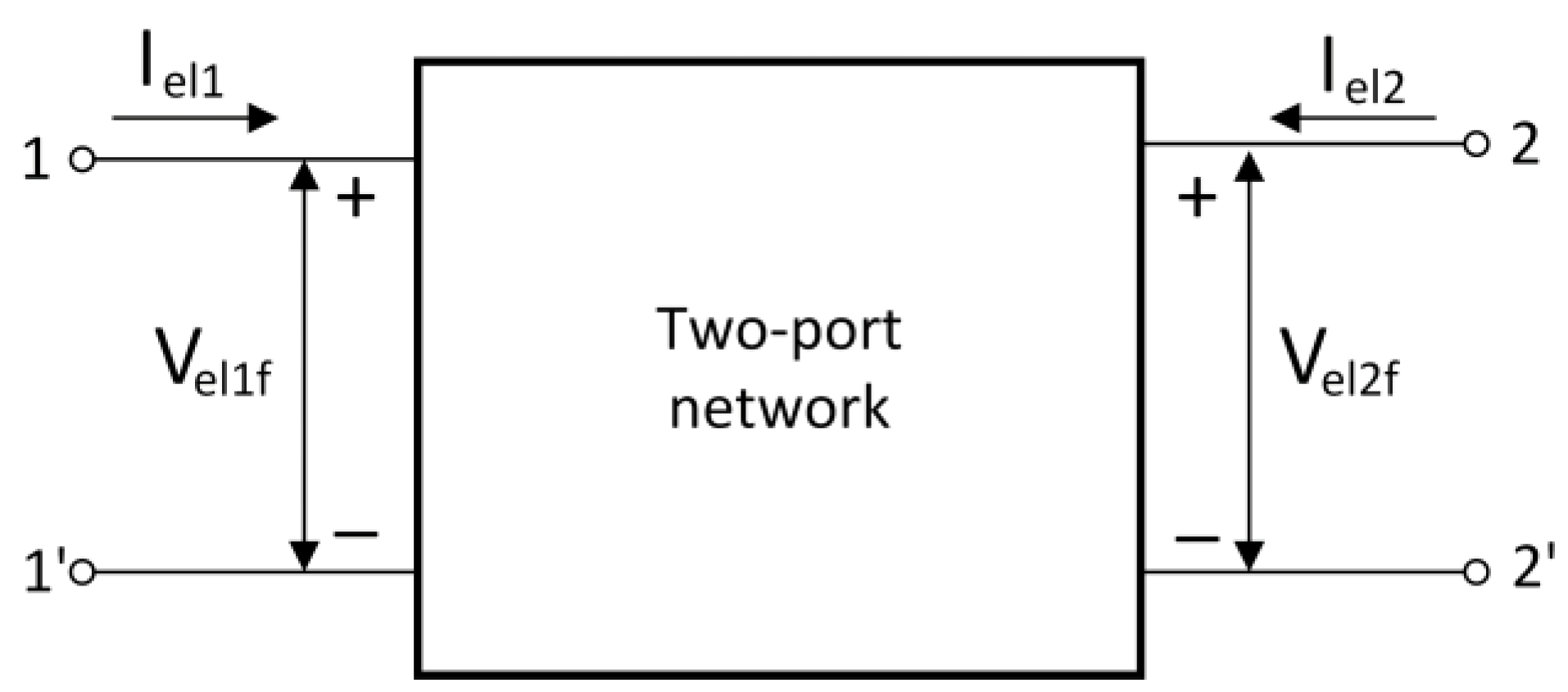
- Vel-ext1—compressor’s voltage at the suction side;
- Pel-ext1—compressor’s active power at the suction side;
- Pel-ext2—compressor’s active power at the discharge side.
2.3. Gas Pressure Reducing and Metering Station
2.4. Gas Pipeline
2.5. Gas Load, Gas Input, Underground Gas Storage
2.6. Power-to-Gas
2.7. Gas-Fired Power Plant
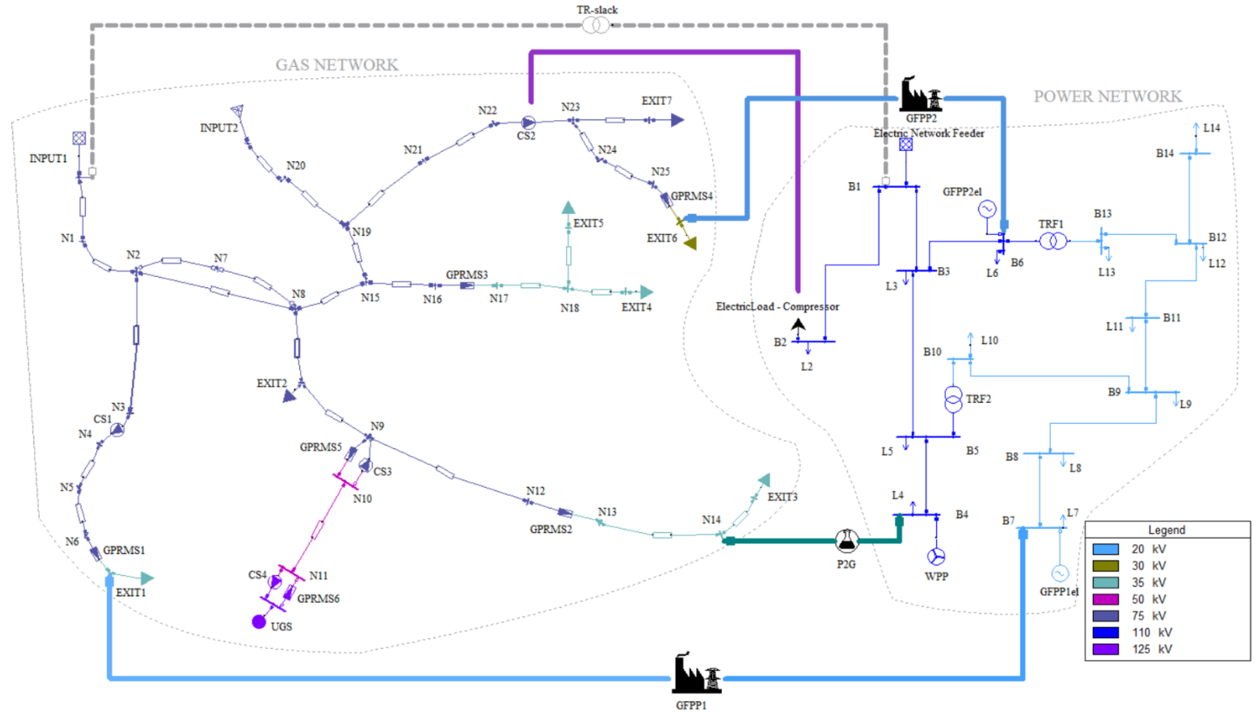
3. Case Studies
3.1. Case Study 1
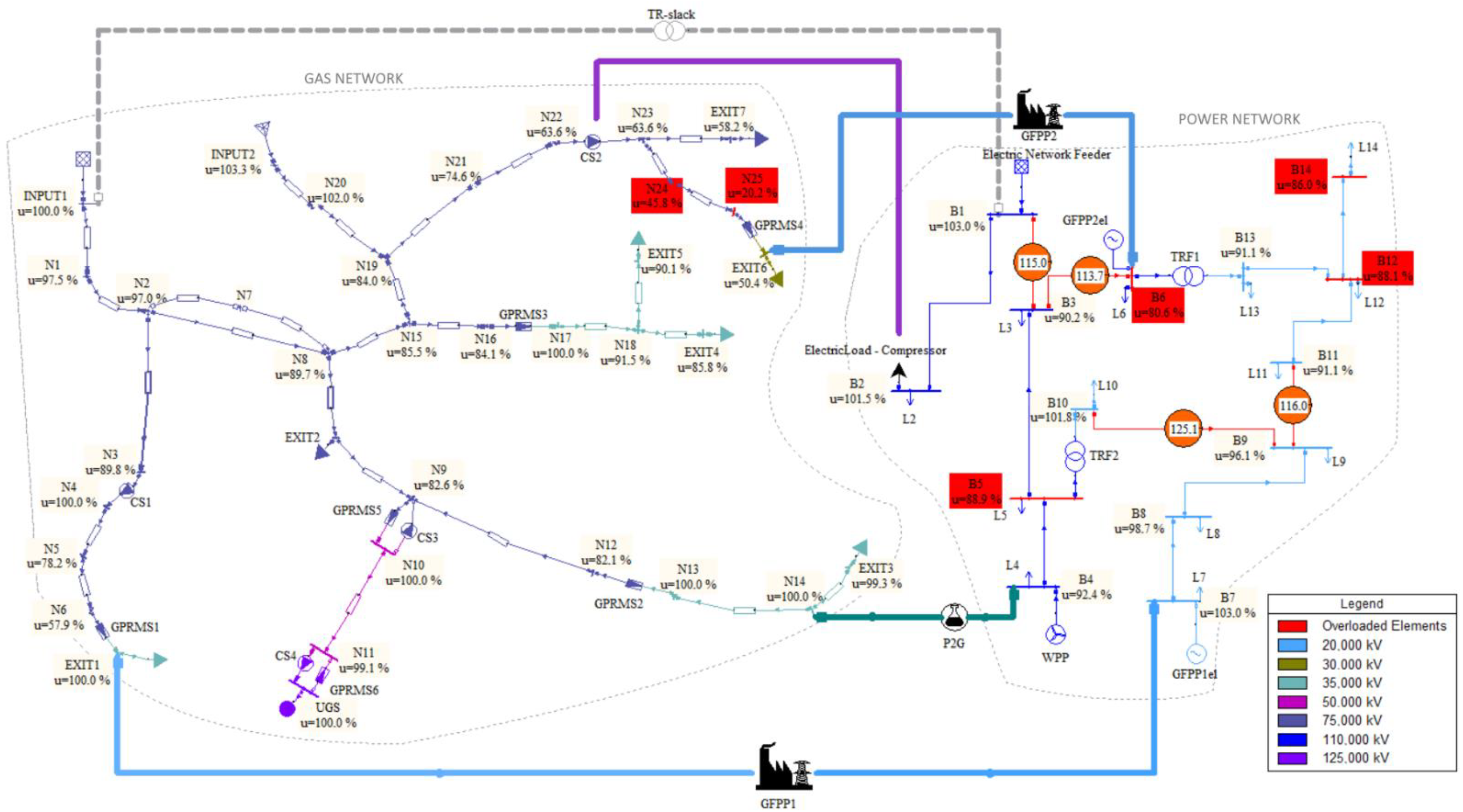
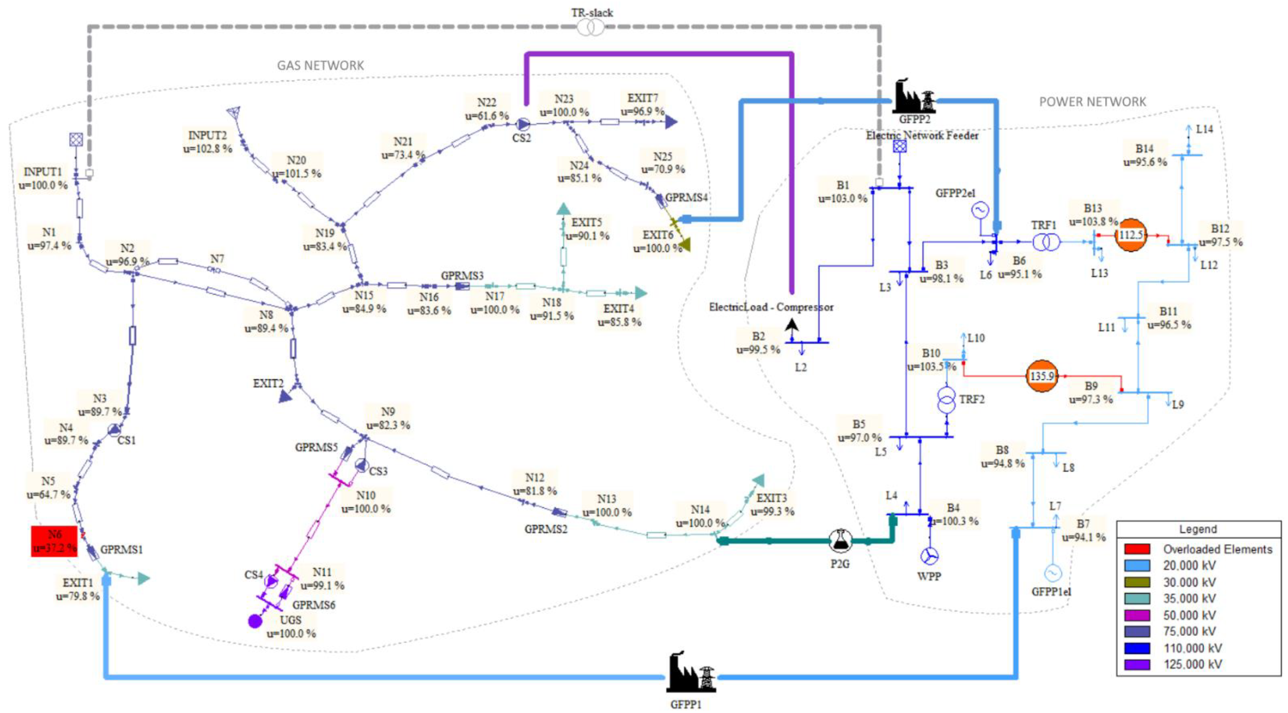
3.2. Case Study 2
- When GFPP1 and GFPP2 were in operation, the most influenced gas nodes were N6 and N25, respectively, (gas pressures were decreased for 0.01 p.u. and 0.088 p.u., respectively). At the same time, the volumetric gas flows at nodes EXIT1 and EXIT6 were increased by 1.1% and 16.4%, respectively, both compared with situations when GFPP1 and GFPP2 were out of operation. The decreased gas pressures of N6 and N25 were still higher than the nominal gas pressures of nodes EXIT1 and EXIT6; therefore, the influences of GFPP1 and GFPP2 on the gas network could be neglected.
- When the P2G was in operation, the most influenced gas node was N12 (gas pressure was decreased by 0.014 p.u.). Interestingly, the volumetric gas flow produced by P2G (0.026 m3/s) was a little higher than the volumetric gas flow at node N14 demanded by EXIT3 (0.022 m3/s). This meant that the losses in the natural gas network could be reduced since natural gas did not need to flow anymore from node N9 to node N14 (130 km). Its flow reached velocities below the minimum allowed (less than 1.5 m/s). Thus, it can be concluded that P2G had a positive influence on the gas network.
4. Conclusions
Author Contributions
Funding
Conflicts of Interest
Abbreviations
| Variables | |
| Ael | voltage angle (rad) |
| D | pipeline diameter (m) |
| E | gas potential energy (Pa) |
| G | gas specific gravity (dimensionless) |
| H | pipeline height (m) |
| HV | heating value (kWh/Nm3) |
| Iel | electric current (A) |
| JT | Joule–Thomson coefficient (°F/100 psi) |
| k0 | gas mass flow consumption by the compressor’s driver (%) |
| k11, k12, k21, k22, k1v2-k6v2 | constant parts of the segmented compressibility factor equation |
| kp | active power setting (W) |
| kpr | constant related to reduced gas pressures in the compressibility factor segmented expression |
| kq | reactive power setting (var) |
| kTr | constant related to reduced gas temperatures in the compressibility factor segmented expression |
| kv | bus voltage setting (%) |
| kVAb | base power (kVA) |
| kVb | base pressure (bar) |
| L | pipeline length (m) |
| mass flow rate (kg/s) | |
| Mw | molecular weight (g/mol) |
| p | absolute gas pressure (Pa) |
| Pel | active power (W) |
| Q | volumetric flow rate (m3/s) |
| Qel | reactive power (var) |
| rc | compression ratio (dimensionless) |
| R | resistance (Ω) |
| Ru | universal gas constant (8.314462618 m3⋅Pa⋅K−1⋅mol−1) |
| T | absolute gas temperature (K) |
| Vel | electric voltage (V) |
| z | gas compressibility factor (dimensionless) |
| Subscripts | |
| 1 | first port, inlet/suction side |
| 2 | second port, outlet/discharge side |
| avg | average |
| const | the constant part of the equation |
| GFPP | gas-fired power plant |
| P2G | power-to-gas |
| p | pipeline |
| r | reduced |
| st | standard conditions |
| Greek Symbols | |
| η | efficiency factor (%) |
| ε | surface roughness (mm) |
| Acronyms | |
| AGA | American Gas Association |
| CS | Compressor Station |
| DLL | Dynamic Link Library |
| ENTSO-E | European Network of Transmission System Operators for Electricity |
| ENTSOG | European Network of Transmission System Operators for Gas |
| GFPP | Gas-Fired Power Plant |
| GPRMS | Gas Pressure Reducing and Metering Station |
| HHV | High Heating Value |
| LHV | Low Heating Value |
| MES | Multi-Energy System |
| P2G | Power-to-Gas |
| PV, PQ | Types in the load flow formulation |
| RES | Renewable Energy Sources |
| SPP | Solar Power Plants |
| TR | Transformer |
| TYNDP | Ten-Year Network Development Plan |
| UDM | User-Defined Models |
| UGS | Underground Gas Storage |
| WPP | Wind Power Plant |
References
- European Commission. A Clean Planet for All a European Strategic Long-Term Vision for a Prosperous, Modern, Competitive and Climate Neutral Economy; European Commission: Luxembourg, 2018. [Google Scholar]
- United Nations. Paris Agreement; United Nations: Geneva, Switzerland, 2015. [Google Scholar]
- European Commission. European Green Deal; European Commission: Luxembourg, 2019. [Google Scholar]
- ENTSOG and ENTSO-E. Ten-Year Network Development Plan 2020; ENTSOG and ENTSO-E: Brussels, Belgium, 2019. [Google Scholar]
- European Commission. An EU Strategy for Energy System Integration; European Commission: Luxembourg, 2020. [Google Scholar]
- European Commission. A Hydrogen Strategy for a Climate-Neutral Europe; European Commission: Luxembourg, 2020. [Google Scholar]
- Mazza, A.; Bompard, E.; Chicco, G. Applications of Power to Gas Technologies in Emerging Electrical Systems. Renew. Sustain. Energy Rev. 2018, 92, 794–806. [Google Scholar] [CrossRef]
- Lewandowska-Bernat, A.; Desideri, U. Opportunities of Power-to-Gas Technology in Different Energy Systems Architectures. Appl. Energy 2018, 228, 57–67. [Google Scholar] [CrossRef]
- He, L.; Lu, Z.; Zhang, J.; Geng, L.; Zhao, H.; Li, X. Low-Carbon Economic Dispatch for Electricity and Natural Gas Systems Considering Carbon Capture Systems and Power-to-Gas. Appl. Energy 2018, 224, 357–370. [Google Scholar] [CrossRef]
- Enerdata EnerOutlook. 2019. Available online: https://eneroutlook.enerdata.net/ (accessed on 13 October 2019).
- Mancarella, P. MES (Multi-Energy Systems): An Overview of Concepts and Evaluation Models. Energy 2014, 65, 1–17. [Google Scholar] [CrossRef]
- Guelpa, E.; Bischi, A.; Verda, V.; Chertkov, M.; Lund, H. Towards Future Infrastructures for Sustainable Multi-Energy Systems: A Review. Energy 2019, 184, 2–21. [Google Scholar] [CrossRef]
- Kleinschmidt, V.; Hamacher, T.; Perić, V.; Hesamzadeh, M.R. Unlocking Flexibility in Multi-Energy Systems: A Literature Review. In Proceedings of the 2020 17th International Conference on the European Energy Market (EEM), Stockholm, Sweden, 16–18 September 2020; ISBN 9781728169194. [Google Scholar]
- Son, Y.-G.; Oh, B.-C.; Acquah, M.A.; Fan, R.; Kim, D.-M.; Kim, S.-Y. Multi Energy System with an Associated Energy Hub: A Review. IEEE Access 2021, 1. [Google Scholar] [CrossRef]
- Li, T.; Eremia, M.; Shahidehpour, M. Interdependency of Natural Gas Network and Power System Security. IEEE Trans. Power Syst. 2008, 23, 1817–1824. [Google Scholar] [CrossRef]
- Urbina, M.; Li, Z. Modeling and Analyzing the Impact of Interdependency between Natural Gas and Electricity Infrastructures. In Proceedings of the 2008 IEEE Power and Energy Society General Meeting—Conversion and Delivery of Electrical Energy in the 21st Century, Pittsburgh, PA, USA, 20–24 July 2008; pp. 1–6. [Google Scholar]
- Devlin, J.; Li, K.; Higgins, P.; Foley, A. The Importance of Gas Infrastructure in Power Systems with High Wind Power Penetrations. Appl. Energy 2016, 167, 294–304. [Google Scholar] [CrossRef] [Green Version]
- Qiao, Z.; Guo, Q.; Sun, H.; Pan, Z.; Liu, Y.; Xiong, W. An Interval Gas Flow Analysis in Natural Gas and Electricity Coupled Networks Considering the Uncertainty of Wind Power. Appl. Energy 2017, 201, 343–353. [Google Scholar] [CrossRef]
- Devlin, J.; Li, K.; Higgins, P.; Foley, A. A Multi Vector Energy Analysis for Interconnected Power and Gas Systems. Appl. Energy 2017, 192, 315–328. [Google Scholar] [CrossRef] [Green Version]
- Correa-Posada, C.M.; Sánchez-Martín, P.; Lumbreras, S. Security-Constrained Model for Integrated Power and Natural-Gas System. J. Mod. Power Syst. Clean Energy 2017, 5, 326–336. [Google Scholar] [CrossRef] [Green Version]
- Zeng, Q.; Zhang, B.; Fang, J.; Chen, Z. A Bi-Level Programming for Multistage Co-Expansion Planning of the Integrated Gas and Electricity System. Appl. Energy 2017, 200, 192–203. [Google Scholar] [CrossRef]
- Qadrdan, M.; Ameli, H.; Strbac, G.; Jenkins, N. Efficacy of Options to Address Balancing Challenges: Integrated Gas and Electricity Perspectives. Appl. Energy 2017, 190, 181–190. [Google Scholar] [CrossRef] [Green Version]
- Cui, H.; Li, F.; Hu, Q.; Bai, L.; Fang, X. Day-Ahead Coordinated Operation of Utility-Scale Electricity and Natural Gas Networks Considering Demand Response Based Virtual Power Plants. Appl. Energy 2016, 176, 183–195. [Google Scholar] [CrossRef] [Green Version]
- Erdener, B.C.; Pambour, K.A.; Lavin, R.B.; Dengiz, B. An Integrated Simulation Model for Analysing Electricity and Gas Systems. Int. J. Electr. Power Energy Syst. 2014, 61, 410–420. [Google Scholar] [CrossRef]
- Pambour, K.; Cakir Erdener, B.; Bolado-Lavin, R.; Dijkema, G. Development of a Simulation Framework for Analyzing Security of Supply in Integrated Gas and Electric Power Systems. Appl. Sci. 2017, 7, 47. [Google Scholar] [CrossRef] [Green Version]
- Pambour, K.A.; Cakir Erdener, B.; Bolado-Lavin, R.; Dijkema, G.P.J. SAInt—A Novel Quasi-Dynamic Model for Assessing Security of Supply in Coupled Gas and Electricity Transmission Networks. Appl. Energy 2017, 203, 829–857. [Google Scholar] [CrossRef]
- Drauz, S.R.; Spalthoff, C.; Würtenberg, M.; Kneikse, T.M.; Braun, M. A Modular Approach for Co-Simulations of Integrated Multi-Energy Systems: Coupling Multi-Energy Grids in Existing Environments of Grid Planning & Operation Tools. In Proceedings of the 2018 Workshop on Modeling and Simulation of Cyber-Physical Energy Systems (MSCPES), Porto, Portugal, 10 April 2018; pp. 1–6. [Google Scholar] [CrossRef]
- Liu, X.; Mancarella, P. Modelling, Assessment and Sankey Diagrams of Integrated Electricity-Heat-Gas Networks in Multi-Vector District Energy Systems. Appl. Energy 2016, 167, 336–352. [Google Scholar] [CrossRef]
- Shabanpour-Haghighi, A.; Seifi, A.R. An Integrated Steady-State Operation Assessment of Electrical, Natural Gas, and District Heating Networks. IEEE Trans. Power Syst. 2016, 31, 3636–3647. [Google Scholar] [CrossRef]
- Zeng, Q.; Fang, J.; Li, J.; Chen, Z. Steady-State Analysis of the Integrated Natural Gas and Electric Power System with Bi-Directional Energy Conversion. Appl. Energy 2016, 184, 1483–1492. [Google Scholar] [CrossRef]
- Awange, J.L.; Paláncz, B. Geospatial Algebraic Computations; Springer International Publishing: New York, NY, USA, 2016; ISBN 9783319254630. [Google Scholar]
- Vidović, D.; Sutlović, E.; Majstrović, M. Steady State Analysis and Modeling of the Gas Compressor Station Using the Electrical Analogy. Energy 2019, 166, 307–317. [Google Scholar] [CrossRef]
- Taherinejad, M.; Hosseinalipour, S.M.; Madoliat, R. Steady Flow Analysis and Modeling of the Gas Distribution Network Using the Electrical Analogy. IJE Trans. B 2014, 27, 1269–1276. [Google Scholar]
- Two-Port Networks. Available online: http://fourier.eng.hmc.edu/e84/lectures/ch2/node4.html (accessed on 7 May 2020).
- Network Theory—Two-Port Networks. Available online: https://www.tutorialspoint.com/network_theory/network_theory_twoport_networks.htm (accessed on 7 May 2020).
- Bakshi, U.A.; Bakshi, A.V. Electrical Network Analysis and Synthesis, 1st ed.; Technical Publications: Maharashtra, India, 2008; ISBN 9788184314618. [Google Scholar]
- Powell, L. Power System Load Flow Analysis; McGraw-Hill Education: New York, NY, USA, 2004; ISBN 0071447792. [Google Scholar]
- Bretas, A.S.; Bretas, N.G.; Braunstein, S.H.; Rossoni, A.; Trevizan, R.D. Multiple Gross Errors Detection, Identification and Correction in Three-Phase Distribution Systems WLS State Estimation: A per-Phase Measurement Error Approach. Electr. Power Syst. Res. 2017, 151, 174–185. [Google Scholar] [CrossRef]
- Rodríguez Paz, M.C.; Ferraz, R.G.; Bretas, A.S.; Leborgne, R.C. System Unbalance and Fault Impedance Effect on Faulted Distribution Networks. Comput. Math. Appl. 2010, 60, 1105–1114. [Google Scholar] [CrossRef] [Green Version]
- Liwacom Informationstechnik GmbH; SIMONE Research Group. Equations and Methods. In SIMONE Software User Manual; Liwacom: Essen, Germany, 2016. [Google Scholar]
- Vidović, D.; Sutlović, E.; Majstrović, M. The Electrical Analogy Model of the Gas Pressure Reducing and Metering Station. Energy 2020, 198, 117342. [Google Scholar] [CrossRef]
- NEPLAN AG. User Defined Models for Load Flow Calculations. In NEPLAN Software User Manual; NEPLAN AG: Küsnacht, Switzerland, 2017; pp. 1–9. [Google Scholar]


| Gas | Formula | Mole Fraction | Molecular Weight (g/mol) | Molecular Weight of Gas Component (g/mol) |
|---|---|---|---|---|
| Methane | CH4 | 95.2% | 16.043 | 15.34 |
| Ethane | C2H6 | 2.29% | 30.07 | 0.69 |
| Propane | C3H8 | 0.63% | 44.096 | 0.28 |
| i-butane | C4H10 | 0.09% | 58.124 | 0.05 |
| Nitrogen | N2 | 1.06% | 28.014 | 0.30 |
| Carbon-dioxide | CO2 | 0.31% | 44.01 | 0.14 |
| Molecular weight of the gas mixture | 16.79 | |||
| UGS | CS1 | CS2 | Scenario |
|---|---|---|---|
| Injection | In operation | In operation | S1 |
| Bypass | In operation | S2 | |
| In operation | Bypass | S3 | |
| Withdrawal | In operation | In operation | S4 |
| Bypass | In operation | S5 | |
| In operation | Bypass | S6 |
| Node 1 | Node 2 | Diameter (mm) | Roughness (mm) | Length (km) | Node 1 Height (m) | Node 2 Height (m) |
|---|---|---|---|---|---|---|
| N18 | EXIT4 | 200 | 0.018 | 10 | 100 | 120 |
| INPUT1 | N1 | 600 | 0.012 | 10 | 0 | 10 |
| N1 | N2 | 600 | 0.012 | 2 | 10 | 10 |
| N17 | N18 | 200 | 0.018 | 5 | 4 | 100 |
| N2 | N8 | 600 | 0.012 | 70 | 10 | 10 |
| N13 | N14 | 150 | 0.012 | 30 | 80 | 80 |
| N18 | EXIT5 | 200 | 0.018 | 5 | 100 | 80 |
| N14 | EXIT3 | 150 | 0.012 | 5 | 80 | 150 |
| N20 | N19 | 200 | 0.03 | 50 | 25 | 50 |
| N8 | EXIT2 | 400 | 0.012 | 50 | 10 | 15 |
| INPUT2 | N20 | 200 | 0.012 | 4 | 0 | 25 |
| N21 | N22 | 400 | 0.012 | 20 | 70 | 100 |
| EXIT2 | N9 | 400 | 0.012 | 50 | 15 | 0 |
| N9 | N12 | 150 | 0.012 | 100 | 0 | 80 |
| N23 | EXIT7 | 350 | 0.012 | 10 | 100 | 100 |
| N10 | N11 | 400 | 0.012 | 10 | 0 | 0 |
| N2 | N7 | 350 | 0.015 | 15 | 10 | −10 |
| N7 | N8 | 350 | 0.015 | 20 | −10 | 10 |
| N15 | N19 | 400 | 0.018 | 4 | 30 | 50 |
| N2 | N3 | 500 | 0.012 | 80 | 10 | 20 |
| N23 | N24 | 250 | 0.03 | 20 | 100 | 65 |
| N15 | N16 | 200 | 0.012 | 4.5 | 30 | 4 |
| N8 | N15 | 400 | 0.012 | 10 | 10 | 30 |
| N5 | N6 | 350 | 0.015 | 25 | 100 | 100 |
| N24 | N25 | 250 | 0.01 | 20 | 65 | 0 |
| N4 | N5 | 350 | 0.024 | 32 | 20 | 100 |
| N19 | N21 | 400 | 0.012 | 20 | 50 | 70 |
| Element | Parameter | UGS Injection | UGS Withdrawal | Unit |
|---|---|---|---|---|
| CS1 | Discharge pressure | 75 | 75 | bar |
| CS1 | Discharge temperature | 15 | 15 | °C |
| CS2 | Discharge pressure | 75 | 75 | bar |
| CS2 | Discharge temperature | 20 | 20 | °C |
| CS3 | Compression ratio | Off | 1.5 | - |
| CS3 | Discharge temperature | 10 | 10 | °C |
| CS4 | Discharge pressure | 125 | Off | bar |
| CS4 | Discharge temperature | 10 | 10 | °C |
| EXIT1 | Gas demand | 200 | 200 | 1000 Nm3/h |
| EXIT2 | Gas demand | 35 | 35 | 1000 Nm3/h |
| EXIT3 | Gas demand | 3 | 3 | 1000 Nm3/h |
| EXIT4 | Gas demand | 20 | 20 | 1000 Nm3/h |
| EXIT5 | Gas demand | 15 | 15 | 1000 Nm3/h |
| EXIT6 | Gas demand | 77 | 77 | 1000 Nm3/h |
| EXIT7 | Gas demand | 155 | 155 | 1000 Nm3/h |
| GPRMS1 | Discharge pressure | 35 | 35 | bar |
| GPRMS1 | Discharge temperature | 10 | 10 | °C |
| GPRMS2 | Discharge pressure | 35 | 35 | bar |
| GPRMS2 | Discharge temperature | 10 | 10 | °C |
| GPRMS3 | Discharge pressure | 35 | 35 | bar |
| GPRMS3 | Discharge temperature | 10 | 10 | °C |
| GPRMS4 | Discharge pressure | 30 | 30 | bar |
| GPRMS4 | Discharge temperature | 18 | 18 | °C |
| GPRMS5 | Discharge pressure | 30 | Off | bar |
| GPRMS5 | Discharge temperature | 10 | 10 | °C |
| GPRMS6 | Suction pressure | Off | 125 | bar |
| GPRMS6 | Discharge temperature | 10 | 10 | °C |
| INPUT1 | Pressure set | 75 | 75 | Bar |
| INPUT1 | Gas temperature | 10 | 10 | °C |
| INPUT2 | Gas supply | 35 | −15 | 1000 Nm3/h |
| INPUT2 | Gas temperature | 10 | 10 | °C |
| UGS | Gas demand | 80 | −150 | 1000 Nm3/h |
| Node | S1-N | S1-S | S2-N | S2-S | S3-N | S3-S | S4-N | S4-S | S5-N | S5-S | S6-N | S6-S |
|---|---|---|---|---|---|---|---|---|---|---|---|---|
| EXIT1 | 35.000 | 35.000 | 28.126 | 27.200 | 35.000 | 35.000 | 35.000 | 35.000 | 31.300 | 30.556 | 35.000 | 35.000 |
| EXIT2 | 66.286 | 65.602 | 66.236 | 65.604 | 66.218 | 65.629 | 75.728 | 75.697 | 75.699 | 75.698 | 75.678 | 75.714 |
| EXIT3 | 34.259 | 34.125 | 34.259 | 34.125 | 34.259 | 34.125 | 34.259 | 34.125 | 34.259 | 34.125 | 34.259 | 34.125 |
| EXIT4 | 30.044 | 29.795 | 30.044 | 29.795 | 30.044 | 29.795 | 30.044 | 29.795 | 30.044 | 29.795 | 30.044 | 29.795 |
| EXIT5 | 31.544 | 31.386 | 31.544 | 31.386 | 31.544 | 31.386 | 31.544 | 31.386 | 31.544 | 31.386 | 31.544 | 31.386 |
| EXIT6 | 30.000 | 30.000 | 30.000 | 30.000 | 19.630 | 20.213 | 30.000 | 30.000 | 30.000 | 30.000 | 23.542 | 24.539 |
| EXIT7 | 72.652 | 72.564 | 72.652 | 72.564 | 48.660 | 47.934 | 72.652 | 72.564 | 72.652 | 72.564 | 50.264 | 49.747 |
| INPUT1 | 75.000 | 74.995 | 75.000 | 74.995 | 75.000 | 74.995 | 75.000 | 74.996 | 75.000 | 74.996 | 75.000 | 74.996 |
| INPUT2 | 79.935 | 79.818 | 79.895 | 79.820 | 79.808 | 79.867 | 64.693 | 64.140 | 64.658 | 64.142 | 64.519 | 64.200 |
| N1 | 73.173 | 73.095 | 73.137 | 73.097 | 73.157 | 73.101 | 74.145 | 74.098 | 74.120 | 74.099 | 74.134 | 74.102 |
| N10 | 30.000 | 30.000 | 30.000 | 30.000 | 30.000 | 30.000 | 53.764 | 53.868 | 53.746 | 53.868 | 53.733 | 53.878 |
| N11 | 29.163 | 29.053 | 29.163 | 29.053 | 29.163 | 29.053 | 55.271 | 55.445 | 55.253 | 55.446 | 55.241 | 55.455 |
| N12 | 63.256 | 62.108 | 63.204 | 62.110 | 63.185 | 62.136 | 79.478 | 79.484 | 79.451 | 79.485 | 79.432 | 79.500 |
| N13 | 35.000 | 35.000 | 35.000 | 35.000 | 35.000 | 35.000 | 35.000 | 35.000 | 35.000 | 35.000 | 35.000 | 35.000 |
| N14 | 34.524 | 34.410 | 34.524 | 34.410 | 34.524 | 34.410 | 34.524 | 34.410 | 34.524 | 34.410 | 34.524 | 34.410 |
| N15 | 67.042 | 66.579 | 66.994 | 66.581 | 66.912 | 66.629 | 68.701 | 68.369 | 68.669 | 68.370 | 68.569 | 68.414 |
| N16 | 66.118 | 65.589 | 66.069 | 65.591 | 65.985 | 65.641 | 67.811 | 67.418 | 67.778 | 67.419 | 67.676 | 67.464 |
| N17 | 35.000 | 35.000 | 35.000 | 35.000 | 35.000 | 35.000 | 35.000 | 35.000 | 35.000 | 35.000 | 35.000 | 35.000 |
| N18 | 32.026 | 31.914 | 32.026 | 31.914 | 32.026 | 31.914 | 32.026 | 31.914 | 32.026 | 31.914 | 32.026 | 31.914 |
| N19 | 66.041 | 65.538 | 65.991 | 65.540 | 65.885 | 65.598 | 67.220 | 66.841 | 67.187 | 66.842 | 67.055 | 66.897 |
| N2 | 72.814 | 72.721 | 72.770 | 72.723 | 72.794 | 72.729 | 73.985 | 73.930 | 73.956 | 73.931 | 73.971 | 73.934 |
| N20 | 78.992 | 78.833 | 78.951 | 78.834 | 78.864 | 78.882 | 64.740 | 64.209 | 64.706 | 64.211 | 64.568 | 64.268 |
| N21 | 59.797 | 58.963 | 59.742 | 58.965 | 59.478 | 59.087 | 61.108 | 60.427 | 61.071 | 60.429 | 60.779 | 60.539 |
| N22 | 52.696 | 51.417 | 52.633 | 51.420 | 52.163 | 51.625 | 54.193 | 53.114 | 54.151 | 53.115 | 53.652 | 53.299 |
| N23 | 75.000 | 75.000 | 75.000 | 75.000 | 52.163 | 51.623 | 75.000 | 75.000 | 75.000 | 75.000 | 53.652 | 53.297 |
| N24 | 67.012 | 66.875 | 67.012 | 66.875 | 38.193 | 38.234 | 67.012 | 66.875 | 67.012 | 66.875 | 40.247 | 40.549 |
| N25 | 59.969 | 59.454 | 59.969 | 59.454 | 19.630 | 20.214 | 59.969 | 59.454 | 59.969 | 59.454 | 23.542 | 24.540 |
| N3 | 67.669 | 67.259 | 67.317 | 67.274 | 67.648 | 67.267 | 68.937 | 68.578 | 68.606 | 68.590 | 68.922 | 68.583 |
| N4 | 75.000 | 75.000 | 67.317 | 67.272 | 75.000 | 75.000 | 75.000 | 75.000 | 68.606 | 68.587 | 75.000 | 75.000 |
| N5 | 58.981 | 58.715 | 48.612 | 48.521 | 58.981 | 58.715 | 58.981 | 58.715 | 50.423 | 50.376 | 58.981 | 58.715 |
| N6 | 44.199 | 43.392 | 28.126 | 27.201 | 44.199 | 43.390 | 44.199 | 43.392 | 31.300 | 30.557 | 44.199 | 43.390 |
| N7 | 71.692 | 71.528 | 71.647 | 71.530 | 71.653 | 71.543 | 0.000 | 0.000 | 0.000 | 0.000 | 0.000 | 0.000 |
| N8 | 69.945 | 69.615 | 69.899 | 69.617 | 69.881 | 69.640 | 72.792 | 72.608 | 72.762 | 72.609 | 72.741 | 72.626 |
| N9 | 64.485 | 63.540 | 64.434 | 63.543 | 64.414 | 63.568 | 80.645 | 80.801 | 80.618 | 80.802 | 80.599 | 80.817 |
| UGS | 125.000 | 125.000 | 125.000 | 125.000 | 125.000 | 125.000 | 125.000 | 125.000 | 125.000 | 125.000 | 125.000 | 125.000 |
| Node | S1-N | S1-S | S2-N | S2-S | S3-N | S3-S | S4-N | S4-S | S5-N | S5-S | S6-N | S6-S |
|---|---|---|---|---|---|---|---|---|---|---|---|---|
| EXIT1 | 1.448 | 1.448 | 1.832 | 1.898 | 1.448 | 1.448 | 1.448 | 1.448 | 1.633 | 1.658 | 1.448 | 1.448 |
| EXIT2 | 0.296 | 0.306 | 0.297 | 0.306 | 0.297 | 0.305 | 0.451 | 0.449 | 0.452 | 0.449 | 0.452 | 0.449 |
| EXIT3 | 0.022 | 0.022 | 0.022 | 0.022 | 0.022 | 0.022 | 0.022 | 0.022 | 0.022 | 0.022 | 0.022 | 0.022 |
| EXIT4 | 0.171 | 0.172 | 0.171 | 0.172 | 0.171 | 0.172 | 0.171 | 0.172 | 0.171 | 0.172 | 0.171 | 0.172 |
| EXIT5 | 0.121 | 0.122 | 0.121 | 0.122 | 0.121 | 0.122 | 0.121 | 0.122 | 0.121 | 0.122 | 0.121 | 0.122 |
| EXIT6 | 0.682 | 0.682 | 0.682 | 0.682 | 1.067 | 1.029 | 0.682 | 0.682 | 0.682 | 0.682 | 0.881 | 0.844 |
| EXIT7 | 0.499 | 0.500 | 0.499 | 0.500 | 0.782 | 0.795 | 0.499 | 0.500 | 0.499 | 0.500 | 0.754 | 0.763 |
| INPUT1 | 1.707 | 1.716 | 1.725 | 1.715 | 1.715 | 1.713 | 1.148 | 1.154 | 1.166 | 1.153 | 1.157 | 1.151 |
| INPUT2 | 0.101 | 0.101 | 0.101 | 0.101 | 0.101 | 0.101 | 0.055 | 0.056 | 0.055 | 0.056 | 0.055 | 0.056 |
| N1 | 1.756 | 1.767 | 1.775 | 1.766 | 1.764 | 1.763 | 1.164 | 1.170 | 1.182 | 1.169 | 1.172 | 1.167 |
| N10 | 0.684 | 0.697 | 0.684 | 0.697 | 0.684 | 0.697 | 0.677 | 0.676 | 0.678 | 0.676 | 0.678 | 0.676 |
| N11 | 0.705 | 0.722 | 0.705 | 0.722 | 0.705 | 0.722 | 0.657 | 0.655 | 0.657 | 0.655 | 0.657 | 0.654 |
| N12 | 0.011 | 0.012 | 0.011 | 0.012 | 0.011 | 0.012 | 0.009 | 0.009 | 0.009 | 0.009 | 0.009 | 0.009 |
| N13 | 0.022 | 0.022 | 0.022 | 0.022 | 0.022 | 0.022 | 0.022 | 0.022 | 0.022 | 0.022 | 0.022 | 0.022 |
| N14 | 0.022 | 0.022 | 0.022 | 0.022 | 0.022 | 0.022 | 0.022 | 0.022 | 0.022 | 0.022 | 0.022 | 0.022 |
| N15 (N16) | 0.123 | 0.124 | 0.123 | 0.124 | 0.124 | 0.124 | 0.120 | 0.121 | 0.120 | 0.121 | 0.120 | 0.121 |
| N15 (N19) | 0.694 | 0.703 | 0.695 | 0.703 | 0.705 | 0.699 | 0.847 | 0.855 | 0.847 | 0.855 | 0.858 | 0.851 |
| N15 (N8) | 0.818 | 0.828 | 0.818 | 0.828 | 0.829 | 0.823 | 0.967 | 0.975 | 0.967 | 0.975 | 0.978 | 0.971 |
| N16 | 0.125 | 0.126 | 0.125 | 0.126 | 0.126 | 0.126 | 0.122 | 0.123 | 0.122 | 0.123 | 0.122 | 0.122 |
| N17 | 0.253 | 0.253 | 0.253 | 0.253 | 0.253 | 0.253 | 0.253 | 0.253 | 0.253 | 0.253 | 0.253 | 0.253 |
| N18 (EXIT4) | 0.159 | 0.160 | 0.159 | 0.160 | 0.159 | 0.160 | 0.159 | 0.160 | 0.159 | 0.160 | 0.159 | 0.160 |
| N18 (EXIT5) | 0.120 | 0.120 | 0.120 | 0.120 | 0.120 | 0.120 | 0.120 | 0.120 | 0.120 | 0.120 | 0.120 | 0.120 |
| N18 (N17) | 0.279 | 0.280 | 0.279 | 0.280 | 0.279 | 0.280 | 0.279 | 0.280 | 0.279 | 0.280 | 0.279 | 0.280 |
| N19 (N15) | 0.706 | 0.716 | 0.707 | 0.716 | 0.717 | 0.712 | 0.868 | 0.877 | 0.869 | 0.877 | 0.880 | 0.873 |
| N19 (N20) | 0.125 | 0.127 | 0.126 | 0.127 | 0.126 | 0.126 | 0.053 | 0.053 | 0.053 | 0.053 | 0.053 | 0.053 |
| N19 (N21) | 0.832 | 0.842 | 0.832 | 0.842 | 0.843 | 0.838 | 0.815 | 0.824 | 0.816 | 0.824 | 0.827 | 0.820 |
| N2 (N1) | 1.766 | 1.777 | 1.785 | 1.776 | 1.774 | 1.774 | 1.166 | 1.173 | 1.185 | 1.172 | 1.175 | 1.170 |
| N2 (N3) | 0.642 | 0.644 | 0.661 | 0.643 | 0.642 | 0.644 | 0.630 | 0.632 | 0.649 | 0.631 | 0.631 | 0.632 |
| N2 (N7) | 0.290 | 0.292 | 0.291 | 0.292 | 0.293 | 0.291 | 0.000 | 0.000 | 0.000 | 0.000 | 0.000 | 0.000 |
| N2 (N8) | 0.833 | 0.842 | 0.834 | 0.842 | 0.839 | 0.839 | 0.536 | 0.541 | 0.536 | 0.541 | 0.544 | 0.538 |
| N20 | 0.102 | 0.103 | 0.102 | 0.103 | 0.103 | 0.103 | 0.055 | 0.056 | 0.055 | 0.056 | 0.055 | 0.055 |
| N21 | 0.930 | 0.949 | 0.931 | 0.949 | 0.946 | 0.943 | 0.908 | 0.923 | 0.908 | 0.923 | 0.924 | 0.917 |
| N22 | 1.071 | 1.106 | 1.073 | 1.106 | 1.096 | 1.096 | 1.039 | 1.066 | 1.039 | 1.066 | 1.062 | 1.058 |
| N23 (EXIT7) | 0.509 | 0.509 | 0.509 | 0.509 | 0.724 | 0.758 | 0.509 | 0.492 | 0.509 | 0.492 | 0.702 | 0.707 |
| N23 (N24) | 0.253 | 0.253 | 0.253 | 0.253 | 0.372 | 0.377 | 0.253 | 0.253 | 0.253 | 0.253 | 0.360 | 0.364 |
| N24 | 0.272 | 0.272 | 0.272 | 0.272 | 0.524 | 0.506 | 0.272 | 0.272 | 0.272 | 0.272 | 0.495 | 0.475 |
| N25 | 0.308 | 0.311 | 0.308 | 0.311 | 1.067 | 1.001 | 0.308 | 0.311 | 0.308 | 0.311 | 0.881 | 0.816 |
| N3 | 0.698 | 0.703 | 0.721 | 0.702 | 0.698 | 0.703 | 0.683 | 0.688 | 0.706 | 0.687 | 0.683 | 0.688 |
| N4 | 0.639 | 0.639 | 0.721 | 0.715 | 0.639 | 0.639 | 0.639 | 0.639 | 0.706 | 0.699 | 0.639 | 0.639 |
| N5 | 0.814 | 0.818 | 1.010 | 1.012 | 0.814 | 0.819 | 0.814 | 0.818 | 0.970 | 0.954 | 0.814 | 0.819 |
| N6 | 1.122 | 1.145 | 1.832 | 1.898 | 1.122 | 1.145 | 1.122 | 1.145 | 1.633 | 1.626 | 1.122 | 1.145 |
| N7 | 0.296 | 0.297 | 0.296 | 0.297 | 0.298 | 0.296 | 0.000 | 0.000 | 0.000 | 0.000 | 0.000 | 0.000 |
| N8 (EXIT2) | 0.397 | 0.404 | 0.397 | 0.404 | 0.397 | 0.404 | 0.360 | 0.359 | 0.360 | 0.359 | 0.360 | 0.358 |
| N8 (N15) | 0.779 | 0.787 | 0.780 | 0.787 | 0.789 | 0.783 | 0.906 | 0.911 | 0.906 | 0.911 | 0.915 | 0.908 |
| N8 (N2) | 0.872 | 0.884 | 0.873 | 0.884 | 0.879 | 0.882 | 0.546 | 0.552 | 0.546 | 0.552 | 0.555 | 0.549 |
| N8 (N7) | 0.304 | 0.307 | 0.304 | 0.307 | 0.307 | 0.306 | 0.000 | 0.000 | 0.000 | 0.000 | 0.000 | 0.000 |
| N9 (EXIT2) | 0.306 | 0.317 | 0.306 | 0.317 | 0.306 | 0.317 | 0.420 | 0.417 | 0.420 | 0.417 | 0.420 | 0.417 |
| N9 (N12) | 0.011 | 0.011 | 0.011 | 0.011 | 0.011 | 0.011 | 0.009 | 0.009 | 0.009 | 0.009 | 0.009 | 0.009 |
| UGS | 0.139 | 0.139 | 0.139 | 0.139 | 0.139 | 0.139 | 0.261 | 0.261 | 0.261 | 0.261 | 0.261 | 0.261 |
| Node 1 | Node 2 | Resistance (Ω) | Reactance (Ω) | Susceptance (μS) | Conductivity (μS) | Rated Current (A) | Length (km) |
|---|---|---|---|---|---|---|---|
| B1 | B2 | 0.164 | 0.338 | 3.456 | 0 | 450 | 50 |
| B1 | B3 | 0.164 | 0.338 | 3.456 | 0 | 450 | 50 |
| B3 | B6 | 0.164 | 0.338 | 3.456 | 0 | 450 | 50 |
| B4 | B5 | 0.164 | 0.338 | 3.456 | 0 | 450 | 50 |
| B5 | B3 | 0.164 | 0.338 | 3.456 | 0 | 450 | 50 |
| B8 | B7 | 0.3 | 0.41 | 2.011 | 0 | 290 | 5 |
| B8 | B9 | 0.3 | 0.41 | 2.011 | 0 | 290 | 5 |
| B9 | B10 | 0.3 | 0.41 | 2.011 | 0 | 290 | 5 |
| B9 | B11 | 0.3 | 0.41 | 2.011 | 0 | 290 | 5 |
| B12 | B11 | 0.3 | 0.41 | 2.011 | 0 | 290 | 5 |
| B12 | B14 | 0.3 | 0.41 | 2.011 | 0 | 290 | 5 |
| B13 | B12 | 0.3 | 0.41 | 2.011 | 0 | 290 | 5 |
| Name | Active Power (MW) | Reactive Power (Mvar) |
|---|---|---|
| L2 | 20 | 2 |
| L3 | 10 | 2 |
| L4 | 16 | 3 |
| L5 | 15 | 2 |
| L6 | 60 | 5 |
| L7 | 1.5 | 0.2 |
| L8 | 3 | 1 |
| L9 | 6 | 1 |
| L10 | 12 | 2.5 |
| L11 | 3 | 1 |
| L12 | 6 | 2 |
| L13 | 15 | 3 |
| L14 | 3.5 | 1 |
| Name | Vector Group | Rated Power (MW) | Rated Primary Voltage (kV) | Rated Secondary Voltage (kV) | Short-Circuit Voltage (%) | Copper Losses (%) | Open-Circuit Current (%) | Iron Core Losses (kW) |
|---|---|---|---|---|---|---|---|---|
| TRF1 | YNd5 | 40 | 110 | 20 | 17.59 | 0.25 | 0.51 | 20.2 |
| TRF2 | YNd5 | 40 | 110 | 20 | 17.59 | 0.25 | 0.51 | 20.2 |
| TR-slack | YNd5 | 80 | 110 | 75 | 17.59 | 0 | 0 | 0 |
Publisher’s Note: MDPI stays neutral with regard to jurisdictional claims in published maps and institutional affiliations. |
© 2021 by the authors. Licensee MDPI, Basel, Switzerland. This article is an open access article distributed under the terms and conditions of the Creative Commons Attribution (CC BY) license (https://creativecommons.org/licenses/by/4.0/).
Share and Cite
Vidović, D.; Sutlović, E.; Majstrović, M. A Unique Electrical Model for the Steady-State Analysis of a Multi-Energy System. Energies 2021, 14, 5753. https://doi.org/10.3390/en14185753
Vidović D, Sutlović E, Majstrović M. A Unique Electrical Model for the Steady-State Analysis of a Multi-Energy System. Energies. 2021; 14(18):5753. https://doi.org/10.3390/en14185753
Chicago/Turabian StyleVidović, Danko, Elis Sutlović, and Matislav Majstrović. 2021. "A Unique Electrical Model for the Steady-State Analysis of a Multi-Energy System" Energies 14, no. 18: 5753. https://doi.org/10.3390/en14185753
APA StyleVidović, D., Sutlović, E., & Majstrović, M. (2021). A Unique Electrical Model for the Steady-State Analysis of a Multi-Energy System. Energies, 14(18), 5753. https://doi.org/10.3390/en14185753