The Ability of a Soil Temperature Gradient-Based Methodology to Detect Leaks from Pipelines in Buried District Heating Channels

Abstract

We carried out several numerical experiments to analyze how different boundary conditions affect the ability to detect small pipeline leaks. Our method is based on determining the soil temperature gradient above a buried district heating channel. The equivalent thermal conductivity of a wet insulation (λ_eq) value of 0.5 W/(m·K) was used to mimic a small water leakage. To evaluate the heat loss through the channel cross section, the heat conduction model was used for the pipe insulation, the concrete, and the soil, while the convection model was considered within the channel. The following effects were used to simulate different operating conditions: heat convection at the soil surface, leakage only from the supply or return pipe, soil height above the channel, soil thermal conductivity, and pipe diameter. With the exception of leakage only from the return pipe and low soil thermal conductivity 0.4 W/(m·K), the results showed a doubling of the soil temperature gradient when compared with the no-leakage case. This fact undoubtedly confirms the potential of the method, which is particularly suitable for leak detection in old pipelines that have priority for renovation. A key added value of this research is that the soil temperature gradient-based leak detection technique was found useful in most foreseeable DH operating situations.

1. Introduction

The purpose of this article is to examine the possibility of detecting small water leaks from district heating (DH) pipes in buried concrete channels under various operating conditions. The research relates to the district heating system of Ljubljana, where about 130 km of such pipelines, most of which are over 50 years old, are installed. In the period from 2005 to 2009 heat loss in the network pipeline was 16.1% of the total heat input. This value is similar to 17% as reported in [1]. We deal with the insulation condition, which is still considered a key parameter in methodologies for evaluating heat losses in DH networks, e.g., [2]. Minimizing losses in the DH network is also an important activity to meet the requirements of the fourth-generation district heating (4GDH) concept [3]. Within this concept, leakage detection and elimination has been highlighted as an important measure [4]. In view of the above, it is necessary to highlight the renovation of old pipelines where leakage is not unusual. Successful detection of small leaks and their remediation certainly helps to achieve the target value about 4% of heat losses in the network pipeline of modern district heating systems, achieved above all by the reduction of supply and return temperature [5]. According to the 4GDH concept, a reduction in heat demand and heat density leads to higher relative heat losses in the heating network [6,7]. These can be reduced by reducing the supply temperature, for which well-maintained piping is a necessity. In this context, upgrading the system by considering the fifth-generation district heating and cooling (5GDHC) concept would be very advantageous [8]. Regardless of the concept, this renovation is associated with high investment costs [9] but is important not only to minimize heat loss but also to reduce additional pressure drops in the network.

A number of studies using the numerical simulation of the temperature field have been carried out to identify pipeline heat loss in a buried channel with dry [10,11,12] or wet pipeline insulation [13,14]. In this study, we used a numerical procedure that was presented in detail and validated by an experiment in our previous work [15], a leak detection methodology based on the determination of the soil temperature gradient above the channel was found to be successful. The research motivation of the present study was to verify the robustness of the method. Ten simulation cases were performed to determine how different boundary conditions influence the soil temperature gradient in the case of a pipeline leak. This was carried out with λ_eq = 0.5 W/(m·K) to imitate the thermal conductivity of the wet insulation [15]. The variation of the operating parameters, including the heat transfer coefficient at ground level, leakage only from the supply pipe, soil height above the channel, soil thermal conductivity, and the diameter of the pipeline, showed a doubling of the soil temperature gradient in the case of wet insulation. A smaller gradient increase was found in two cases: (1) a 40% gradient increase due to return pipe leak only and (2) an 80% gradient increase due to low soil thermal conductivity, λ_s = 0.4 W/(m·K).

The key contribution of this work was to confirm that the detection of small water leaks from pipes in buried district heating channels is possible for most foreseeable DH operating situations. Leak detection requires suitable experimental implementation to control the heat loss through the soil [16,17]. For this purpose, only temperature sensors are required (for example, the use of a digital pyrometer) [18]. The presented methodology can also serve as a supplement to infrared thermography, one of the most promising leakage detection techniques for district heating networks [19].

The article is written as follows. In Section 2, the importance of detecting and dealing with small leaks in DH networks is discussed in more detail. The organization of numerical simulations is given in Section 3. Firstly, governing equations, computational domain with discretization, material properties, boundary conditions, and numerical solutions for computations are presented. Secondly, grounds for the selection of simulation cases are stated. Results are collected and discussed in Section 4 including the reliability of leakage detection. The conclusions are summarized in Section 5.

2. Significance of Small Leakage Detection in DH Networks

Based on our measurements [20], the equivalent thermal conductivity of the insulation along the pipe was determined to be within 0.8 and 1 W/(m·K) at a leak volume flow rate of 500 kg/h. Based on our previous experience [15], λ_eq = 0.5 W/(m·K) was used in the numerical experiments presented in this paper to imitate a leakage below 500 kg/h, which undoubtedly can be defined as a small leak. The selected λ_eq value can be considered appropriate to obtain a leakage detection limit that is as low as possible. Since we consider pipelines that are mostly older than 50 years, such leaks are an inevitable fact. However, the eligibility for renovation is always in question as it is associated with relatively high costs. As discussed in [21], there are four parameters that are not in favor of the current investment in larger district heating systems: (1) reduced heat demand due to building renovation, leading to the relative increase in the pipeline heat loss, (2) high cost of DH transmission and the distribution network, (3) different business strategies between facility operators and energy distributors, and (4) the use of fossil fuels for heat generation. Let us present the problems of the second parameter in more detail: (a) the calculation of the additional heat loss due to leakage, including the loss due to water runoff into the surroundings, and (b) the determination of the distributed heat to obtain a rough estimate of the renovation cost.

(a) The average nominal diameter (DN) of the channel pipe in our case was determined to be 200 mm [10]. For our basic numerical computation [15] (DN 200, soil thermal conductivity λ_s = 0.8 W/(m·K), soil height H_s = 0.9 m), the linear heat loss per meter of pipe was calculated to be 125.9 W/m (60.8 W/m for dry insulation and an additional 65.1 W/m due to leakage). Additionally, it was estimated that 1.5% of the total heat input (1231 GWh in 2009) was lost due to water runoff into the surroundings [10]. Distributed over 130 km of pipeline in channels, the runoff corresponds to 0.142 MWh/m of heat loss in one year. Recalculated as the linear heat loss, this is 16.2 W/m. The sum of all contributions, 142.1 W/m, represents a 2.34-fold increase of the heat loss compared to that for dry insulation. Furthermore, these heat radiation effects (emissivity ε = 0.93 for the cardboard cover roof of the pipe insulation) can cause a roughly 20% increase of the soil temperature gradient [15]. The insulation is no longer functional in any case and thus needs to be replaced. However, since small leaks are difficult to trace, DH companies usually solve the problem by gradually replacing old pipelines, as is the case in Ljubljana [22].

(b) Following the procedure in [21], the distributed heat flux Q is calculated by the equation Q = ρ_wv_wAc_p,wΔθ_w, where ρ_w and v_w are the density and average velocity of water, respectively, A is the internal cross section of the pipe, c_p,w is the specific heat of water, and Δθ_w is the difference between supply and return temperature. For the case of a DN 200 pipe (for the average water velocity of 0.9 m/s [23]), the distributed heat flux was calculated to be 4.75 MW. The pipes in the concrete channels are usually replaced with pre-insulated pipes. The price of a single pipe system can be considered 640 EUR per meter [24]. Although this price means a high investment return time, there are additional advantages: (i) installing piping of the higher insulation class (22% reduction of the distribution heat loss [25]), (ii) a reduction of the chemical water treatment costs, and (iii) a reduction of water pumping costs. The leak elimination helps to achieve the required pressure at the DH end points.

3. Numerical Simulations

3.1. Governing Equations

The modeling of heat transfer in a heating network numerically represents a 3D problem (see e.g., [26]). Since in our case we considered a part of a straight channel segment, few meters long in the vicinity of a leak, we assumed that flow and temperature of water in the pipeline are constant. Due to this, we simplified the problem and treated it as a 2D example.

Two-dimensional transient-steady-state-combined (TSC) simulations [15] represent a basis for the numerical model used to evaluate the heat transfer across the channel cross section. The natural convection in the channel and the heat transfer through the solids is governed by the following [27]:

• Continuity equation:

∂ρ/∂t + ∇·(ρu) = 0;

(1)

• Momentum equation:

∂(ρu)/∂t + ∇·(ρuu) = −∇p + ∇·[μ(∇u + ∇u^T − ⅔∇·uI)] + ρg;

(2)

• Energy equation:

∂(ρE)/∂t + ∇·[u(ρE + p)] = ∇·(λ∇T), E = c_pT − p/ρ + ½u²;

(3)

• Equation of state:

p = ρrT,

(4)

where u is a velocity vector, ρ is the density, p is the pressure, g is the acceleration due to gravity, μ is the dynamic viscosity, I is the identity matrix, T is the temperature, λ is the thermal conductivity, c_p is the specific heat, and r is the specific gas constant.

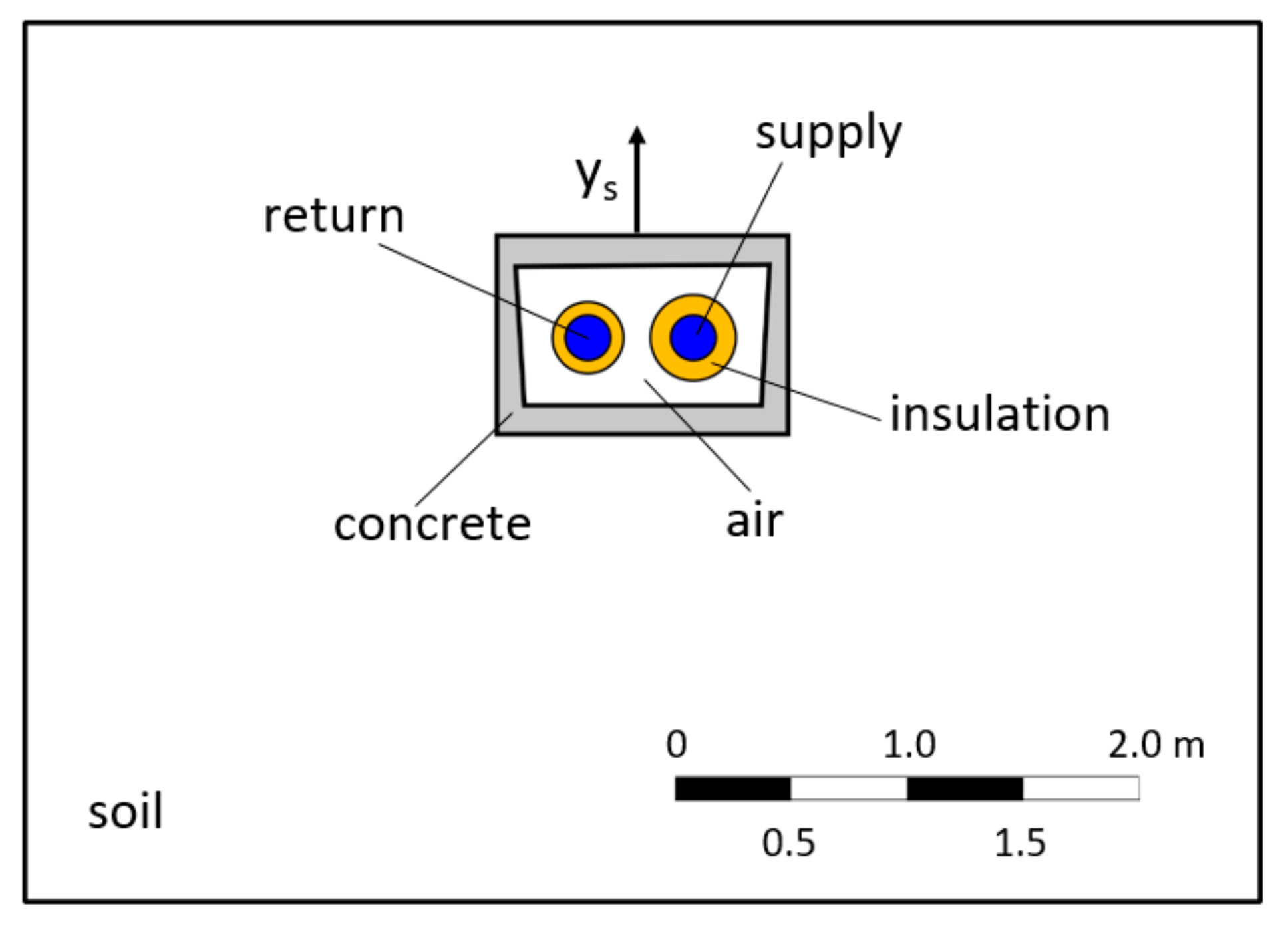
3.2. Computational Domain and Discretization

For the DH system in Ljubljana, the average nominal diameter (DN) of the pipeline in the channel was determined to be 200 mm [10]. Consequently, the configuration of the DN 200 channel was selected as the basic configuration.

Figure 1 shows a computational domain consisting of three solid subdomains (soil, concrete, insulation) and one fluid subdomain (air). The distance between the soil surface and the top of the concrete channel was 0.65 m or 0.9 m. The extension of the soil subdomain was 2 m to the left and right of the concrete channel sides. The same soil subdomain extension was used at the channel’s bottom side. The supply pipe was insulated with 100 mm of glass wool insulation, while the return pipe’s insulation thickness was 50 mm.

The whole computational domain was discretized with 93,793 quadrilateral cells. As in [16], a fine grid was used. In the insulation subdomain, the cell size was 5 mm, while for all other subdomains, the cell size was 50 mm. The mesh quality parameters of the computational grid were as follows:

• Minimum cell orthogonal quality—0.815;
• Maximum cell ortho skew—0.185;
• Maximum cell aspect ratio—2.671.

The values of the mesh quality parameters mean that the computational grid was good and would not be the cause of problems in the numerical solution.

3.3. Material Properties and Boundary Conditions

Air was used as the working fluid to enable convective heat transfer between the pipe insulation and the concrete wall of the channel. The physical properties of the materials used in the numerical simulation are:

• Air—density ρ from the equation of state for an ideal gas, specific heat c_p = 1006 J/(kg·K), thermal conductivity λ = 0.024 W/(m·K), dynamic viscosity μ = 1.789 × 10⁻⁵ kg/(m·s), specific gas constant r = 287.058 J/(kg·K);
• Steel—ρ = 8030 kg/m³, c_p = 502.5 J/(kg·K), λ = 16.27 W/(m·K);
• Concrete—ρ = 2000 kg/m³, c_p = 879 J/(kg·K), λ = 1.14 W/(m·K);
• Soil—ρ = 1800 kg/m³, c_p = 880 J/(kg·K), λ = 0.8 W/(m·K);
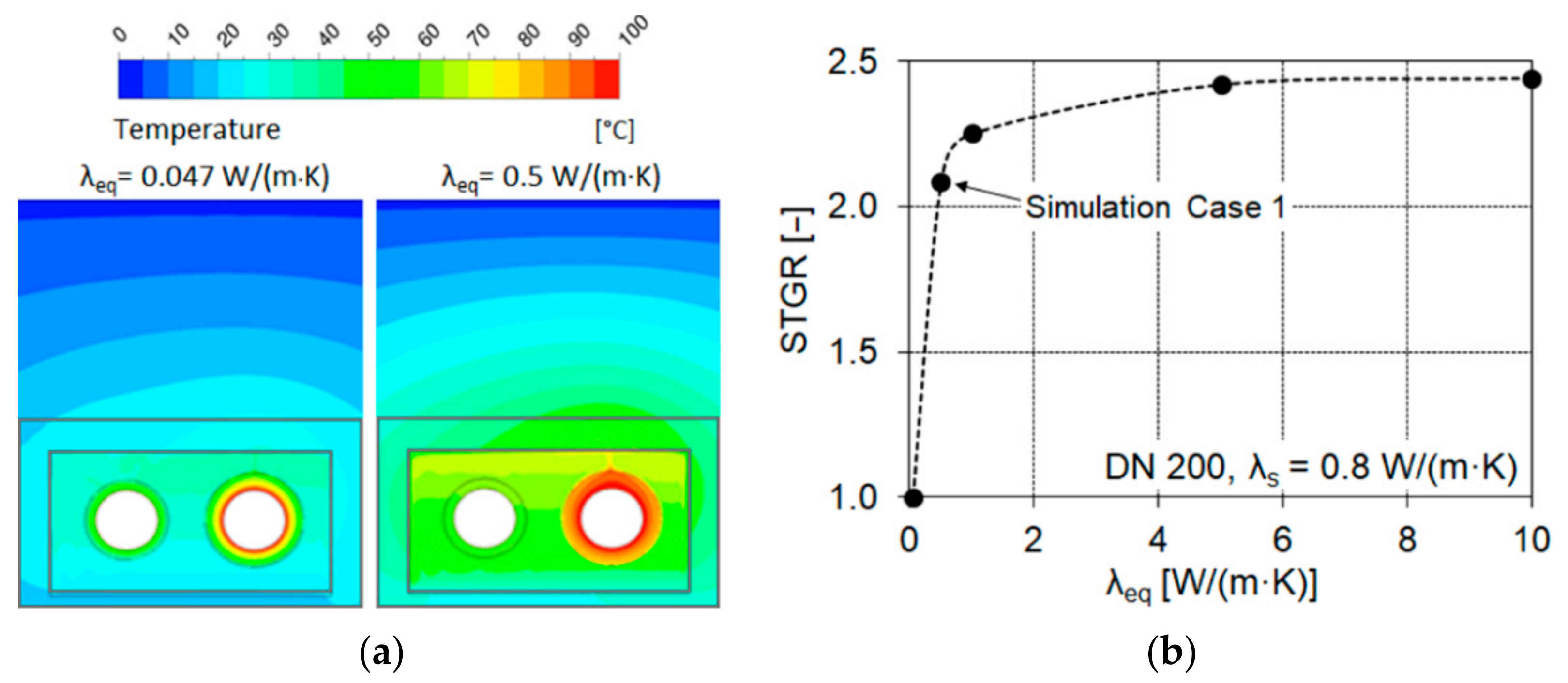
• Insulation—ρ = 20 kg/m³, c_p = 840 J/(kg·K), λ = 0.047 W/(m·K) for no-leak case and λ = 0.5 W/(m·K) for leak case.

The mean value of the heat losses simulated per day for the entire year of 2009 corresponded to heat losses on day 304, 31 October [10], which is why the boundary conditions for this day were used in all simulations of the present work. These included the following temperatures:

• 3.7 °C for the soil surface, assumed to be equal to the temperature of surrounding air [16]);
• 10 °C for the soil temperature at the bottom boundary, equal to the undisturbed ground temperature;
• 100 °C for water temperature in the supply pipeline;
• 60 °C for water temperature in the return pipeline.

Simulations also considered the symmetry on the left and right boundaries and the conjugate heat transfer through the solid domains: soil, concrete, and pipe insulation.

As an initial condition for the temperature field in the transient simulation, the result of the calculation of the steady heat conduction for the stated temperature boundary conditions and the resting air was used.

3.4. Computations

The numerical simulations were performed with the ANSYS Fluent 2D solver. The transient calculation was conducted by using a first-order implicit scheme. The assumption regarding the laminar flow regime was based on the fact that the Rayleigh number was between 5.9 × 10⁵ and 1.4 × 10⁶. The SIMPLE (Semi-Implicit Method for Pressure-Linked Equations) solver option for the coupling of velocity and pressure fields was used. Spatial discretization schemes were the following:

• Gradient operator—Green–Gauss-cell-based;
• Pressure—PRESTO (Pressure Staggering Option);
• Density, momentum and energy—second-order upwind.

The relaxation factors were as follows:

• 0.3 for pressure;
• 0.7 for momentum;
• 1.0 for density and energy.

The maximum residuals (convergence criteria) for the iterative procedure were limited to 10⁻¹² for energy equation and 10⁻⁴ for all other equations. The allowed maximum number of iterations within each time step was set to 20. Since the numerical model had already been experimentally checked [15], it was possible to analyze the robustness of the leakage detection method utilizing the numerical experiments.

3.5. Selection of Simulation Cases

Since the consideration of the convection numerical model within the channel already caused about a twofold increase in the soil temperature gradient, the radiation model was not considered in the simulations discussed in this paper. The soil temperature fields above the channel for the basic numerical computation, here called Simulation Case 1, are shown in Figure 2a. The reduced soil temperature equidistance indicates an increase of the temperature gradient in the leakage case (equivalent thermal conductivity of the insulation λ_eq = 0.5 W/(m·K)). The soil temperature gradient ratio (STGR)—a quotient between the leak and no-leak gradient—is shown in Figure 2b as a function of λ_eq. The smoothed line (Microsoft Excel) indicates a strong STGR reduction between λ_eq = 0.5 W/(m·K) and λ_eq = 1.0 W/(m·K). It can be concluded that the more than doubled soil temperature gradient at λ_eq = 0.5 W/(m·K) certainly confirms the choice of this λ_eq value to characterize the leak in all numerical experiments discussed in this work.

To cover most of the variables that occurred during the normal operation of the DH network, nine further simulation cases were carried out. The variables were heat convection at the soil surface, leakage only from the supply or return pipe, soil height above the channel, soil thermal conductivity, and pipe diameter. The different compared operating conditions are shown in

Table 1. Operating conditions for the simulation cases.

Simulation Case	1	2	3	4	5	6	7	8	9	10
Variable
h, W/(m2·K)	‒	11.3		‒	‒	‒	‒	‒	‒	‒
Supply leak only	‒	‒	Yes	‒	‒	‒	‒	‒	‒	‒
Return leak only	‒	‒	‒	Yes	‒	‒	‒	‒	‒	‒
Hs, m	0.9	0.9	0.9	0.9	0.65	0.9	0.65	0.65	0.9	0.9
λs, W/(m·K)	0.8	0.8	0.8	0.8	0.8	0.8	0.4	1.2	0.8	0.8
DN, mm	200	200	200	200	300	300	300	300	50	900

h, heat transfer coefficient at the soil surface; H_s. soil height; λ_s, soil thermal conductivity; DN, nominal pipe diameter.

. Each case included no-leak and leak computations.

4. Results and Discussion

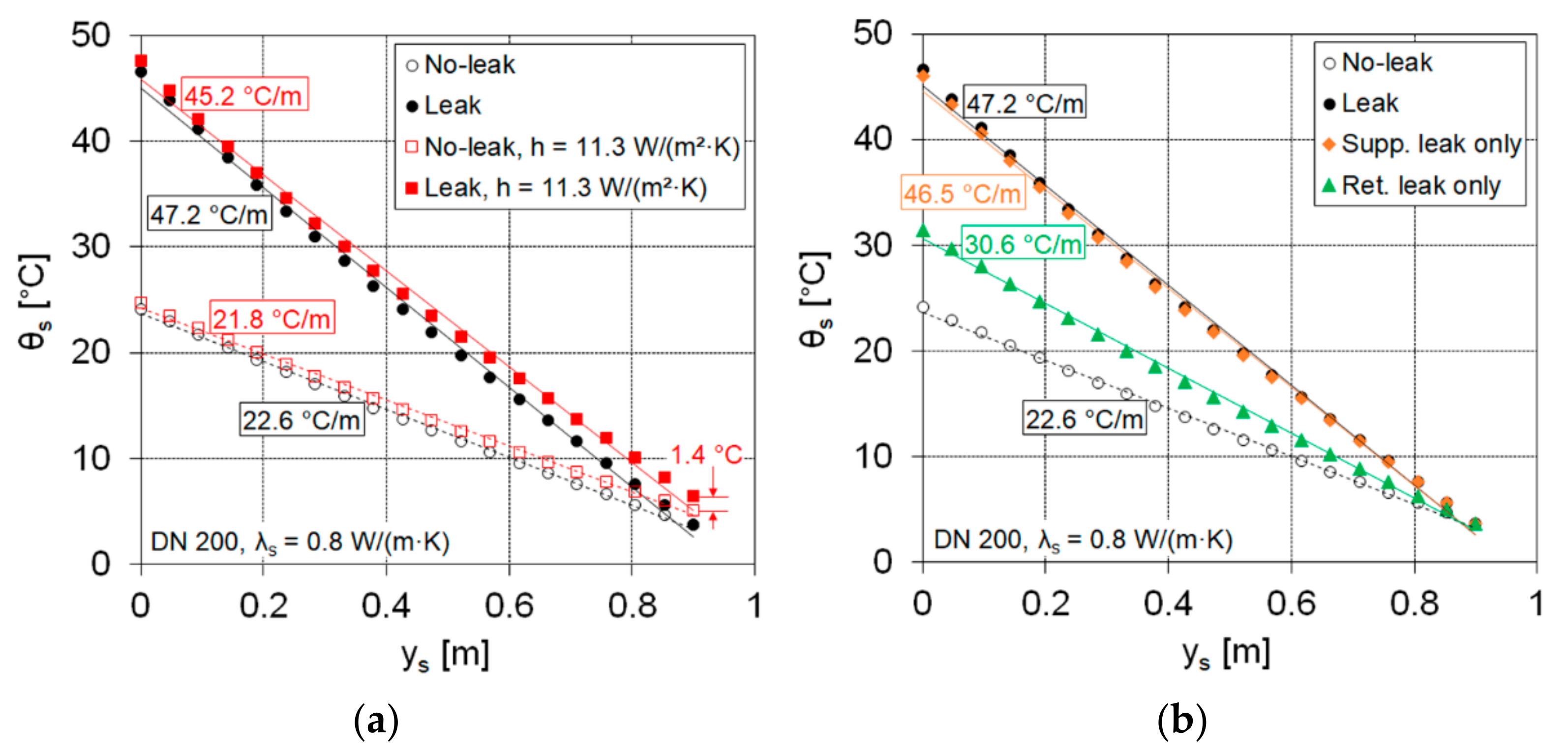
4.1. Heat Convection at the Soil Surface

In [28], a constant value of h = 14.6 W/(m²·K) was taken for the heat transfer coefficient at the soil surface, including convection and radiation. Furthermore, in [11,13,14], a similar value of 15 W/(m²·K) was used for the heat transfer coefficient between the ground and surrounding air. In our previous work [16], the average temperature difference between the air and soil surface was measured in the period of the last three months of 2009 with Δθ = 2 °C. The heat flux density through the soil above the DN 200 channel on the reference day (31 October 2009) was measured at q_s = 22.5 W/m² [10]. From the equation

q_s = hΔθ,

(5)

a heat transfer coefficient at the soil surface of h = 11.3 W/(m²·K), not much lower than the values specified in [11,13,14,28], was calculated. A comparison of the soil temperature profiles simulated for this case with the base case (no-leak and leak) is shown in Figure 3a. A soil temperature gradient was determined via the best linear fit of the temperature profile data. Practically no change of the soil temperature gradient was found if the heat transfer at the soil surface was taken into account. This fact confirms that the soil surface temperature is a sufficient boundary condition [16]. However, as for the base case, more than a twofold increase of the soil temperature gradient was obtained.

It should also be emphasized that the difference in soil surface temperature was only 1.4 °C (see Figure 3a) when comparing the no-leak and leak cases with h = 11.3 W/(m²·K). In this case, utilizing the infrared thermography, it would be very difficult to attribute such a small temperature difference to a leak due to the measurement uncertainty caused by the different ground type (grass, asphalt, concrete). Here, the discussed methodology can certainly be helpful. Heat transfer at the soil surface is also affected by the radiation, e.g., [29]. Since the soil surface temperature was a sufficient boundary condition, the ground radiation effect was disregarded. Consideration of this impact would also significantly increase the computation time.

4.2. Supply or Return Pipe Leak Only

Figure 3b shows the computations for supply or return pipe leaks only. These scenarios are compared with the “Leak” one, representing a leakage from both pipes simultaneously. In the case of a supply pipe leak only, the soil temperature gradient was found not to be much lower than for both a supply and return leak (46.5 °C/m for the supply leak only vs. 47.2 °C/m for the both-pipe leak). It can be argued that for successful leak detection, supply pipe leakage is sufficient. In practice, the supply pipe leak only is more likely than the return pipe leak only due to the higher pressure in the supply pipe. Regardless, the return-pipe-leak case could represent the lower limit of detection since the soil temperature gradient increased by 1.4 times only, from 22.6 °C/m (no-leak) to 30.6 °C/m (leak).

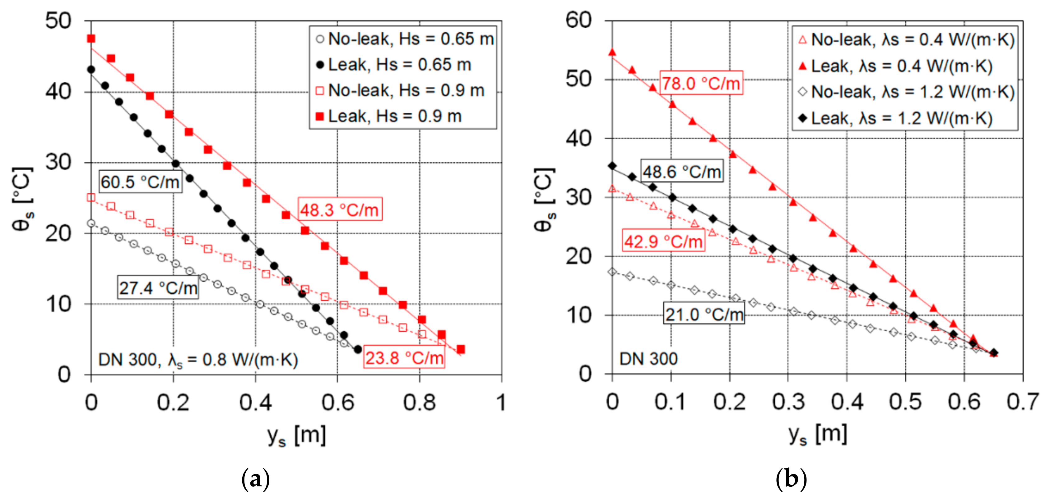
4.3. Soil Height above the Channel

The influence of the soil height was tested for the DN 300 channel. A comparison of the soil temperature profiles is shown in Figure 4a. It can be concluded that the soil height does not play a special role in the leak detection. The increase of the soil temperature gradient compared to the no-leak case was found to be similar for both soil heights, namely 2.2 times for H_s = 0.65 m and 2.0 times for H_s = 0.9 m.

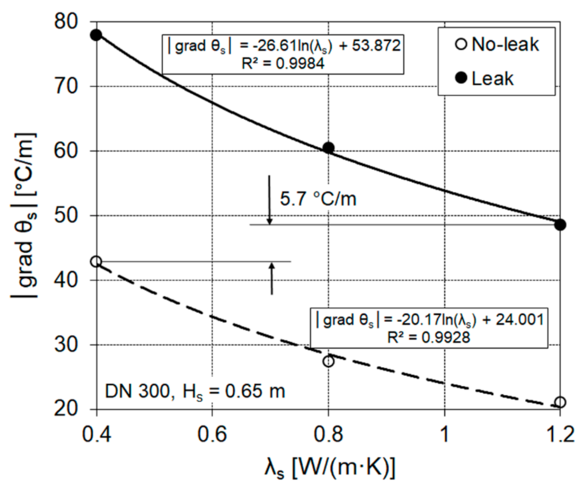
4.4. Soil Thermal Conductivity

For the period from 27 September to 5 November 2009, the mean value of the daily averaged soil thermal conductivity measurements (λ_s) was 0.826 ± 0.085 W/(m·K) [10]. These results are similar to those reported in [30], indicating a soil thermal conductivity in the range from 0.4 W/(m·K) to 1.7 W/(m·K) for sandy loam soil. This is certainly consistent with the fact that the city of Ljubljana is built on sand and gravel alluvium [31]. Based on our measurements, a value of λ_s rounded to 0.8 W/(m·K) was considered in the majority of numerical experiments (Simulation Cases 1‒6, 9, 10). The influence of the soil thermal conductivity was tested via Simulation Cases 7 and 8 (see Figure 4b). The selected λ_s values 0.4 W/(m·K) and 1.2 W/(m·K) correspond to minimal and maximal local value measurements [16]. A lower soil temperature gradient increase was determined for λ_s = 0.4 W/(m·K) than for λ_s = 1.2 W/(m·K), at 1.8 and 2.3 times, respectively. The leak detection problem can arise from the fact that the no-leak gradient at λ_s = 0.4 W/(m·K) is similar to the leak gradient at λ_s = 1.2 W/(m·K), 42.9 °C/m vs. 48.6 °C/m. The issue can be further clarified with the comparison between the no-leak and leak soil temperature gradient |grad θ_s| as a function of the soil thermal conductivity (see Figure 5). The difference of the added constants in the logarithmic trend curves, 29.871 °C/m, shows the average leak vs. no-leak soil temperature gradient difference to be practically independent on λ_s. This means that there is no problem with the leakage detection if λ_s is known; if not, a small difference in the soil temperature gradient between no-leak and leak cases (5.7 °C/m, marked in Figure 5) may lead to an incorrect decision regarding the leak detection. When λ_s, determined as proposed in [16], is 0.4 W/(m·K) or less, the possible leak should be checked by the channel monitoring as proposed in [15]. An additional possibility is to ascertain λ_s via the measured soil heat flux q_s and soil temperature, utilizing the equation

q_s = λ_s |grad θ_s|.

(6)

Although this method, applied in [10], can overestimate λ_s by up to 30%, it can be helpful.

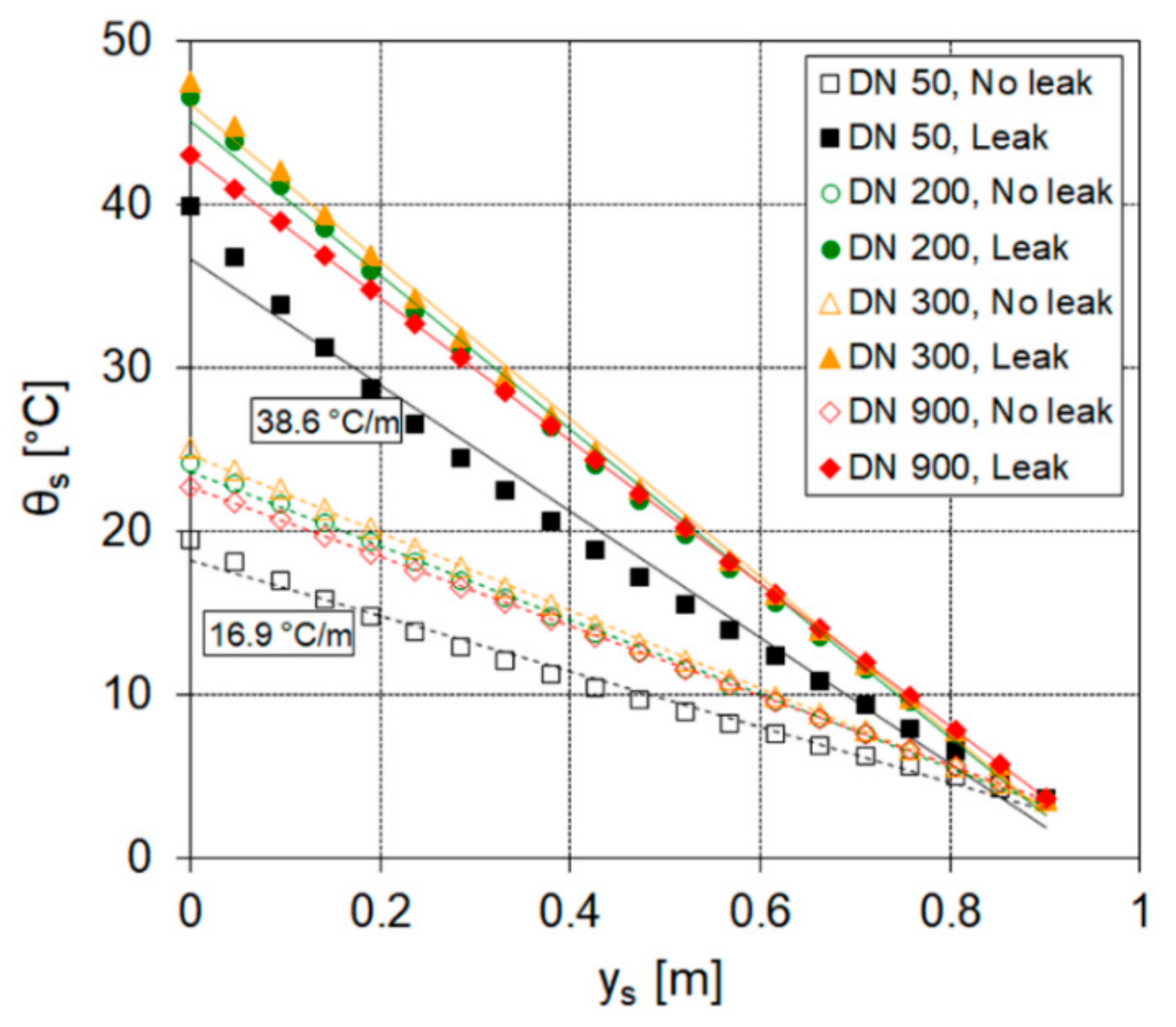
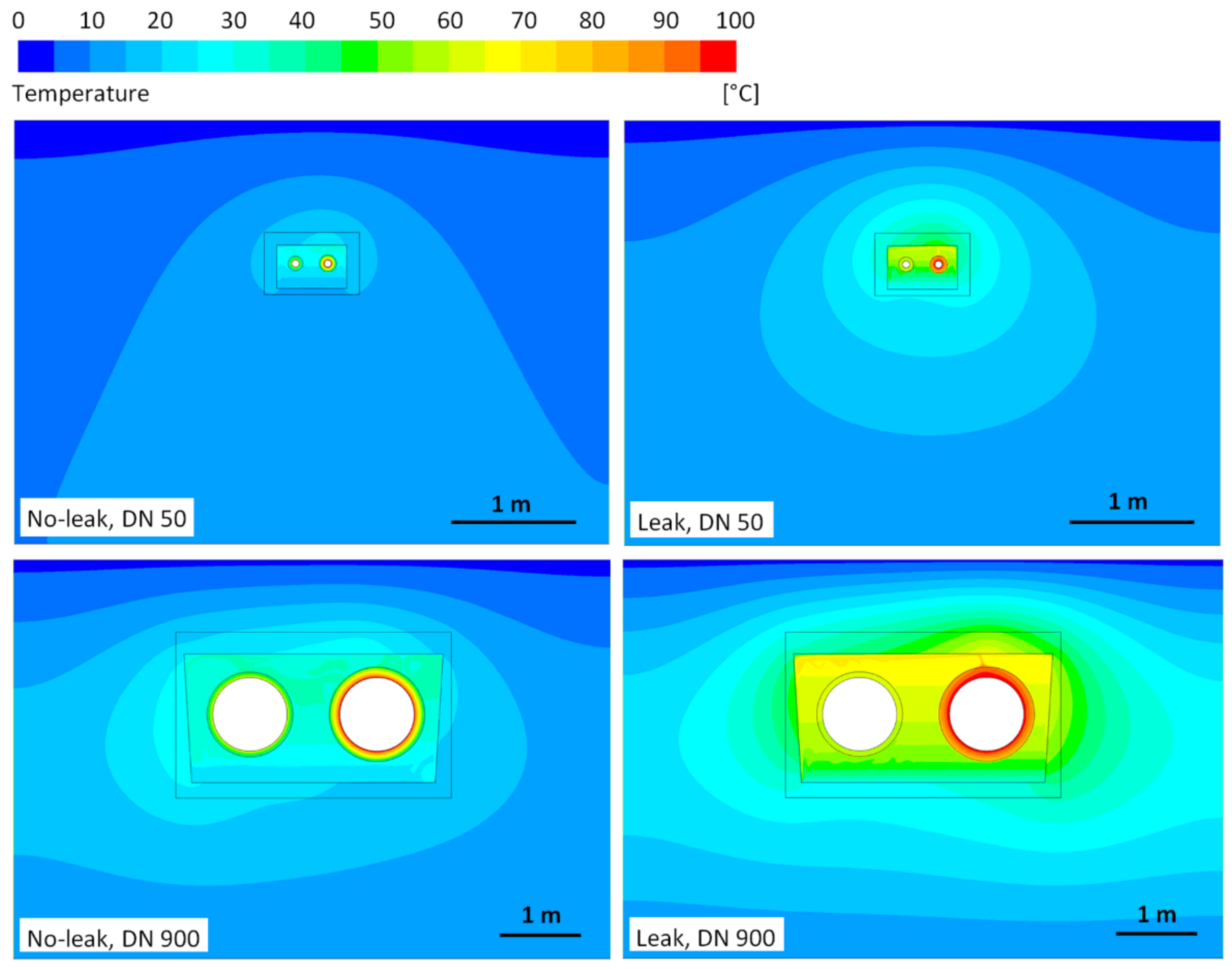
4.5. Channel Dimension

To determine how the channel dimension influences the soil temperature gradient, simulations were carried out for the nominal pipe diameters of 50 mm, 200 mm, 300 mm, and 900 mm (Figure 6). In all cases, the soil height above the channel was 0.9 m. Regardless of the pipe diameter, more than a doubling of the soil temperature gradient was found in the case of leakage. For DN 50, the best fit of the soil temperature data (R² = 0.999) is a quadratic function, but a linear fit with the soil temperature gradient of 38.6 °C/m is also acceptable (R² > 0.98).

Temperature fields related to DN 50 and DN 900 for the no-leak and leak cases are shown in Figure 7. According to the chosen calculation domain, the simulation areas were 4.7 m × 3.4 m for DN 50 and 7.39 × 4.96 m for DN 900.

Although the patterns of isotherms for DN 50 and DN 900 are different, the reduced soil temperature equidistance for the leak cases proves that the presented method can be successfully utilized.

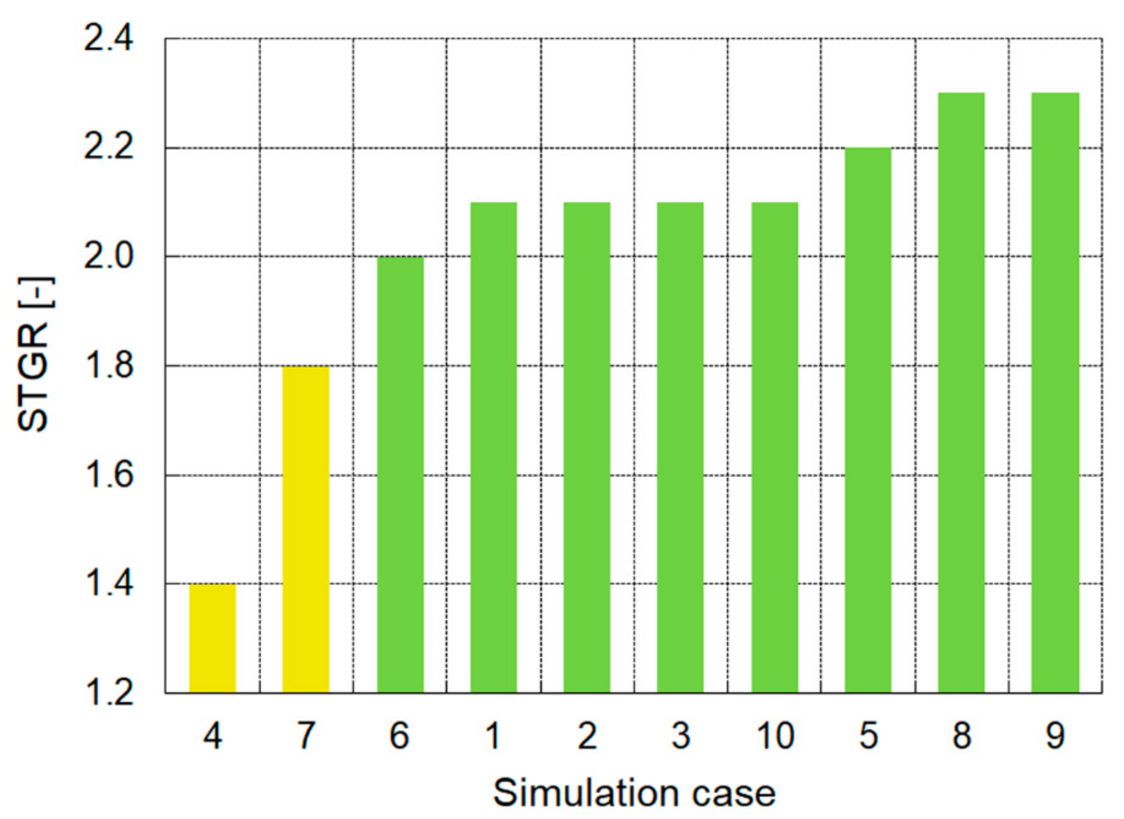
4.6. Reliability of Leakage Detection

The reliability of the leakage detection is shown in Figure 8, where the soil temperature gradient ratios (STGRs) for the considered simulation cases are compared.

Let us emphasize that in [11,13], a more than twofold increase in the soil temperature gradient above the channel was exhibited in the case of heat loss from the pipeline with the wet insulation due to the flooded concrete channel. Based on this fact, a doubling of the soil temperature gradient was taken as a lower limit for reliable leak detection.

STGR values, rounded to one decimal point, are displayed in ascending order (Figure 8). The minimum value (1.4) refers to Simulation Case 4 (return leak only). A somewhat higher STGR (1.8) was found for Simulation Case (low soil thermal conductivity (0.4 W/(m·K)). All other simulation examples met the desired condition of doubling the soil temperature gradient.

5. Conclusions

Different numerical experiments were carried out to analyze the influence of a variety of boundary conditions on the ability of a pipeline leak detection method based on the determination of the soil temperature gradient above a buried district heating channel. The methodology was checked by comparison of simulation and experimental field data [15]. Based on this previous study, the equivalent thermal conductivity of wet insulation (λ_eq) value of 0.5 W/(m·K) was used to mimic a small water leakage into the pipe insulation. The heat loss through the channel cross section was evaluated using the heat conduction model for the pipe insulation, concrete, and soil, while inside the channel the convection model was used. To imitate different operating conditions, the following effects or variables were used in the simulations: heat convection at the soil surface, leakage only from the supply or return pipe, soil height above the channel, soil thermal conductivity, and pipe diameter. The results showed that, with the exception of leakage only at the return and low soil thermal conductivity (0.4 W/(m·K), a doubling of the soil temperature gradient was achieved when compared to the no-leakage case. This fact undoubtedly confirms the potential of the method for detecting small water leaks from the pipelines in buried channels in most foreseeable DH operating situations. The equipment needed are temperature sensors with data recording and control system (e.g., as in [16,17]). In addition to a reduction of heat loss, it is also important to reduce the additional pressure drops in the network. Our proposed method is a useful tool, especially for pipeline renovation planning.

References

1. Volkova, A.; Latõšov, E.; Lepiksaar, K.; Siirde, A. Planning of district heating regions in Estonia. Int. J. Sustain. Energy Plan. Manag. 2020, 27, 5–16. [Google Scholar] [CrossRef]
2. Chicherin, S.; Mašatin, V.; Siirde, A.; Volkova, A. Method for assessing heat loss in a district heating network with a focus on the state of insulation and actual demand for useful energy. Energies 2020, 13, 4505. [Google Scholar] [CrossRef]
3. Lund, H.; Østergaard, P.A.; Chang, M.; Werner, S.; Svendsen, S.; Sorknæs, P.; Thorsen, J.E.; Hvelplund, F.; Mortensen, B.O.G.; Mathiesen, B.V.; et al. The status of 4th generation district heating: Research and results. Energy 2018, 164, 147–159. [Google Scholar] [CrossRef]
4. Li, H.; Nord, N. Transition to the 4th generation district heating—Possibilities, bottlenecks, and challenges. Energy Procedia 2018, 149, 483–498. [Google Scholar] [CrossRef]
5. Zajacs, A.; Borodiņecs, A. Assessment of development scenarios of district heating systems. Sustain. Cities Soc. 2019, 48, 101540. [Google Scholar] [CrossRef]
6. Schweiger, G.; Kuttin, F.; Posch, A. District heating systems: An analysis of strengths, weaknesses, opportunities, and threats of the 4GDH. Energies 2019, 12, 4748. [Google Scholar] [CrossRef] [Green Version]
7. Pakere, I.; Romagnoli, F.; Blumberga, D. Introduction of small-scale 4th generation district heating system. Methodology approach. Energy Procedia 2018, 149, 549–554. [Google Scholar] [CrossRef]
8. Buffa, S.; Cozzini, M.; D’Antoni, M.; Baratieri, M.; Fedrizzi, R. 5th generation district heating and cooling systems: A review of existing cases in Europe. Renew. Sustain. Energy Rev. 2019, 104, 504–522. [Google Scholar] [CrossRef]
9. Sarbu, I.; Mirza, M.; Crasmareanu, E. A review of modelling and optimisation techniques for district heating systems. Int. J. Energy Res. 2019, 43, 6572–6598. [Google Scholar] [CrossRef]
10. Žun, I.; Perpar, M.; Rek, Z.; Gregorc, J. Setting up of Heat Loss Physical Model for DH System in Ljubljana. Report EN10-R7; DH company: Ljubljana, Slovenia, 2010. (In Slovene) [Google Scholar]
11. Kuznetsov, G.V.; Polovnikov, V.Y. The conjugate problem of convective-conductive heat transfer for heat pipelines. J. Eng. Thermophys. 2011, 20, 217–224. [Google Scholar] [CrossRef]
12. Zwierzchowski, R.; Niemyjski, O. Simulation of heat losses of a distribution network with different technical structure and under different operating conditions for a district heating and cooling system. IOP Conf. Ser. Mater. Sci. Eng. 2019, 603, 032091. [Google Scholar] [CrossRef]
13. Polovnikov, V.Y.; Razumov, N.V. Application of a convective-conductive heat transfer model in the heat loss analysis of a heat pipeline under flooding conditions. EPJ Web Conf. 2016, 110, 1–5. [Google Scholar] [CrossRef] [Green Version]
14. Polovnikov, V.Y. Numerical Investigation of the Thermal Regime of Underground Channel Heat Pipelines Under Flooding Conditions with the Use of a Conductive-Convective Heat Transfer Model. J. Eng. Phys. Thermophys. 2018, 91, 471–476. [Google Scholar] [CrossRef]
15. Perpar, M.; Rek, Z. Soil temperature gradient as a useful tool for small water leakage detection from district heating pipes in buried channels. Energy 2020, 201, 117684. [Google Scholar] [CrossRef]
16. Perpar, M.; Rek, Z.; Bajric, S.; Zun, I. Soil thermal conductivity prediction for district heating pre-insulated pipeline in operation. Energy 2012, 44, 197–210. [Google Scholar] [CrossRef]
17. Song, S.; Kim, J.; Detection, L. Advanced Monitoring Technology for District Heating Pipelines Using Fiber Optic Cable. In Proceedings of the 15th International Symposium on District Heating and Cooling, Seoul, Korea, 4–7 September 2016; pp. 1–4. [Google Scholar]
18. Zhuravska, I.; Lernatovych, D.; Burenko, O. Detection the places of the heat energy leak on the underground thermal pipelines using the computer system. Adv. Sci. Technol. Eng. Syst. 2019, 4, 1–9. [Google Scholar] [CrossRef] [Green Version]
19. Zhou, S.; O’Neill, Z.; O’Neill, C. A review of leakage detection methods for district heating networks. Appl. Therm. Eng. 2018, 137, 567–574. [Google Scholar] [CrossRef]
20. Perpar, M.; Lojevec, N.; Gregorc, J.; Rek, Z.; Bajrić, S.; Žun, I. Heat loss evaluation in wet insulation of district heating pipeline in Ljubljana. In Proceedings of the International Conference on District Energy, Portorose, Slovenia, 23–25 March 2014. [Google Scholar]
21. Sandvall, A.F.; Ahlgren, E.O.; Ekvall, T. Cost-efficiency of urban heating strategies—Modelling scale effects of low-energy building heat supply. Energy Strateg. Rev. 2017, 18, 212–223. [Google Scholar] [CrossRef]
22. Matičič, P.; Trunkelj, S. Ensuring high reliability of Energetika Ljubljana district heating systems. In Proceedings of the International Conference on District Energy, Portorose, Slovenia, 19–21 March 2017. [Google Scholar]
23. Žun, I.; Perpar, M.; Polutnik, E.; Rek, Z.; Pečar, M.; Bajrić, S. Setting up of heat loss physical model for DH system in Ljubljana. Report EN06-R3; DH company: Ljubljana, Slovenia, 2006. (In Slovene) [Google Scholar]
24. Danish Energy Agency. Technology Catalogue for Transport of Energy & CO2. 2021. Available online: https://ens.dk/en/our-services/projections-and-models/technology-data/technology-data-energy-transport (accessed on 6 September 2021).
25. Best, I.; Orozaliev, J.; Vajen, K. Impact of Different Design Guidelines on the Total Distribution Costs of 4th Generation District Heating Networks. Energy Procedia 2018, 149, 151–160. [Google Scholar] [CrossRef]
26. Danielewicz, J.; Śniechowska, B.; Sayegh, M.A.; Fidorów, N.; Jouhara, H. Three-dimensional numerical model of heat losses from district heating network pre-insulated pipes buried in the ground. Energy 2016, 108, 172–184. [Google Scholar] [CrossRef] [Green Version]
27. ANSYS® Academic Research CFD, Release 17.2. Available online: https://www.ansys.com/ (accessed on 6 September 2021).
28. Bøhm, B. On transient heat losses from buried district heating pipes. Int. J. Energy Res. 2000, 24, 1311–1334. [Google Scholar] [CrossRef]
29. Bryś, K.; Bryś, T.; Ojrzyńska, H.; Sayegh, M.A.; Głogowski, A. Variability and role of long-wave radiation fluxes in the formation of net radiation and thermal features of grassy and bare soil active surfaces in Wrocław. Sci. Total Environ. 2020, 747, 141192. [Google Scholar] [CrossRef] [PubMed]
30. Ochsner, T.E.; Horton, R.; Ren, T. A New Perspective on Soil Thermal Properties. Soil Sci. Soc. Am. J. 2001, 65, 1641–1647. [Google Scholar] [CrossRef]
31. Soils of Slovenia with Soil Map 1:250,000. ISBN 9789279230639. Available online: http://soil.bf.uni-lj.si/projekti/pdf/atlas_final_2015_reduced.pdf (accessed on 6 September 2021).
Figure 1. Domain geometry, where ys stands for the soil depth.
Energies 14 05712 g001
Figure 2. (a) Computed soil temperature fields above the channel for Simulation Case 1 and (b) soil temperature gradient ratio for different equivalent thermal conductivities of the insulation.
Energies 14 05712 g002
Figure 3. (a) Influence of the convection heat transfer at the soil surface (Simulation Case 2) and (b) influence of the leakage from supply and return pipe only (Simulation Cases 3 and 4).
Energies 14 05712 g003
Figure 4. (a) Influence of the soil height above the channel (Hs = 0.65 m and Hs = 0.9 m refer to Simulation Cases 5 and 6, respectively) and (b) influence of the soil thermal conductivity (λs = 0.4 W/(m·K) and λs = 1.2 W/(m·K) refer to Simulation Cases 7 and 8, respectively).
Energies 14 05712 g004
Figure 5. Comparison of no-leak and leak soil temperature gradients as a function of the soil thermal conductivity.
Energies 14 05712 g005
Figure 6. Influence of the channel dimension. DN 50, DN 200, DN 300, and DN 900 refer to Simulation Cases 9, 1, 6, and 10, respectively.
Energies 14 05712 g006
Figure 7. Simulated temperature fields for channels with nominal pipe diameters DN 50 and DN 900; no-leak and leak cases.
Energies 14 05712 g007
Figure 8. Comparison of the soil temperature gradient ratios (STGRs) for the considered simulation cases.
Energies 14 05712 g008