
Functional Scalability and Replicability Analysis for Smart Grid Functions: The InteGrid Project Approach

 ,
,  , , , , ,
  , , , , ,
Abstract
:1. Introduction
1.1. European Context and Legacy for the Scalabilty and Replicability Analysis
1.2. Research Questions, Key Contributions, and Paper Structure
- How can different scopes such as technical, economic, and regulatory be combined within a unified SRA approach?
- Does clustering of tools for a single SRA bring any benefits compared to conducting an individual SRA of each tool?
- What are the results of the set of tools when facing a scaling process (e.g., increase in RES penetration; network; flexibility offers and device controllability)?
- What are the results of the set of tools when they are exposed to other networks, characteristics, or resources?
- Would other stakeholders be able to replicate the set of tools in their own context?
2. Methodology
2.1. Generic Smart Grid SRA Methodology
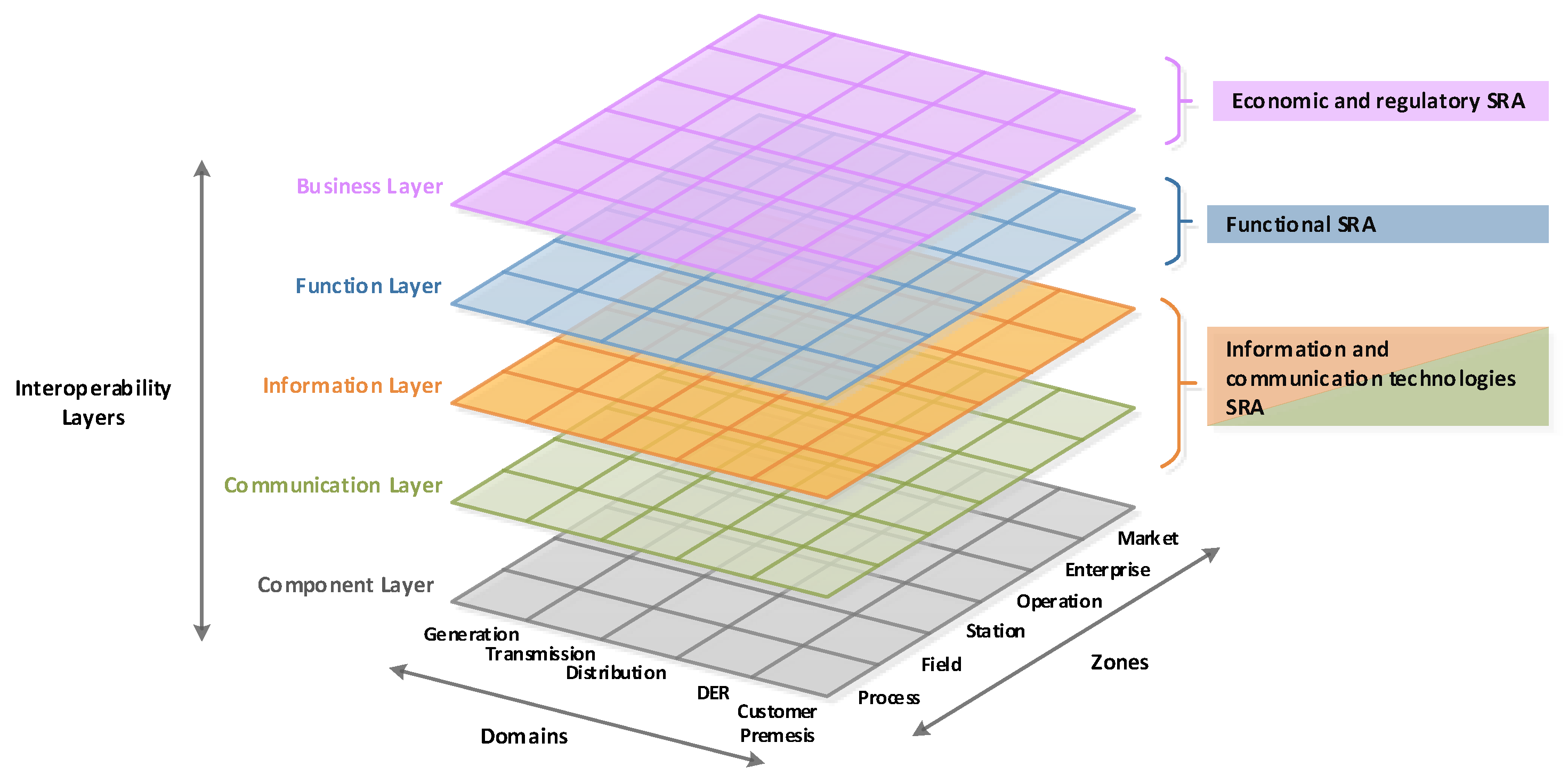
- Functional: validates the technical integration of the smart functions through their impact when integrated within the distribution network while considering the network technical capabilities.
- Information and communication technologies (ICT): provides a system architecture characterization based on the SGAM representation conducted via a qualitative analysis, which identifies the potential bottlenecks and a quantitative analysis which uses stress simulations to evaluate future performance;
- Economic: provides a cost benefit analysis based on the net present value and the initial rate of return of the implementation of the new functions and tools. The analysis gives an overview based on the economies of scale, macroeconomics, and key performance indicators (KPIs);
- Regulatory: investigates the regulatory drivers and barriers which may be imposed within various countries in order to highlight the compatibility of these regulations during the deployment of the smart grid functions.
2.2. Functional Clustering Process
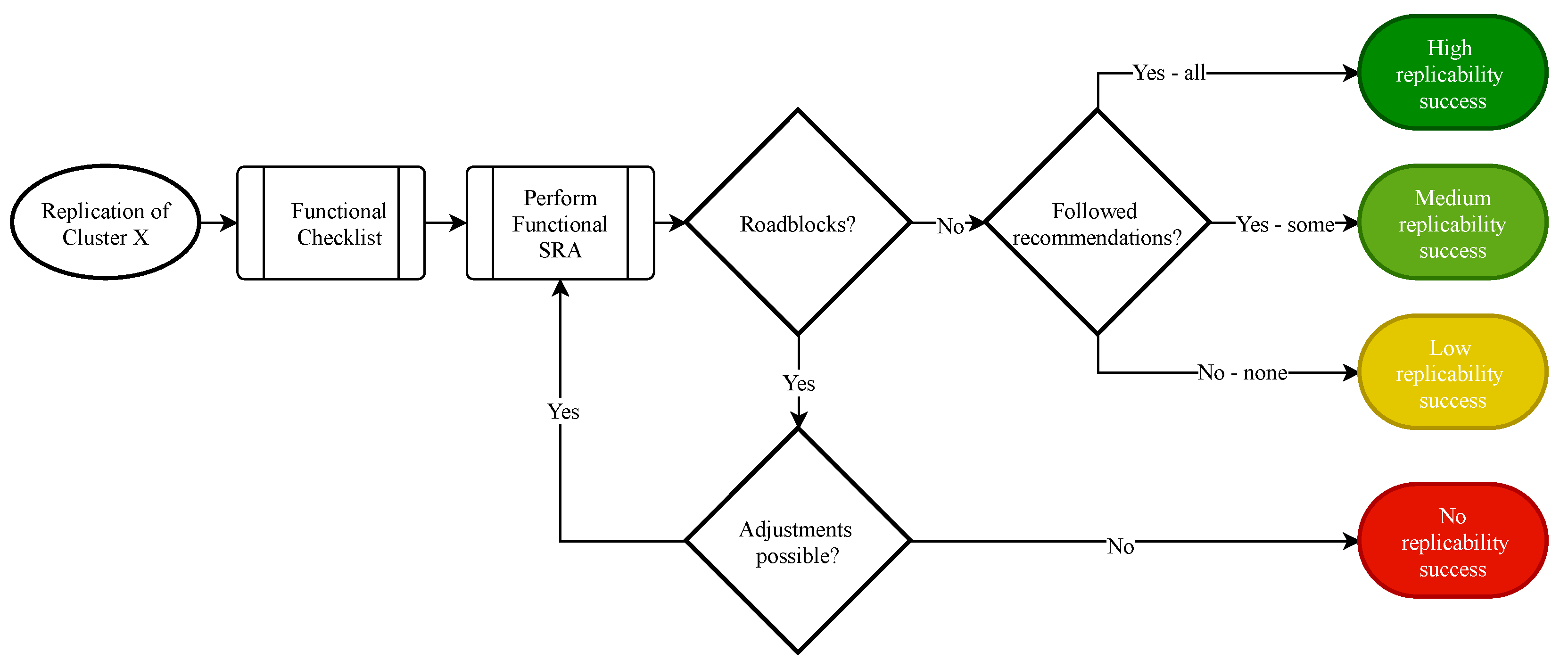
2.3. Functional-Oriented Methodology
3. Case Study: SRA for Portugal
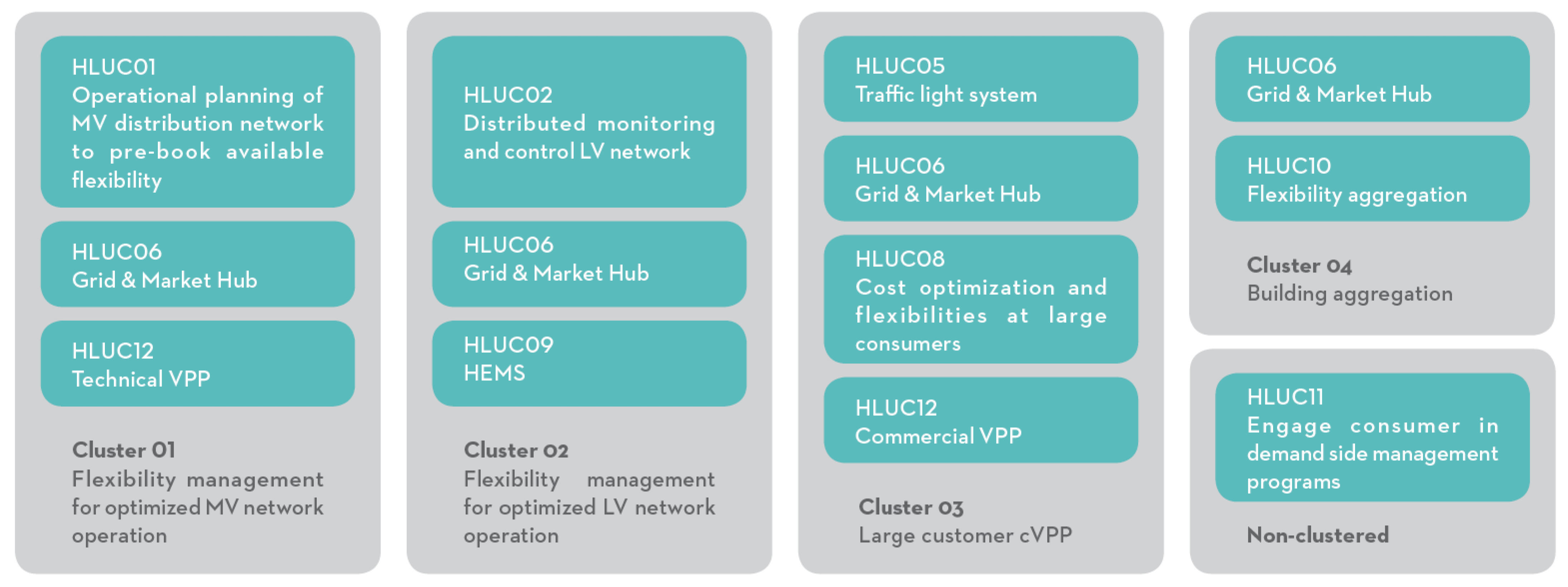
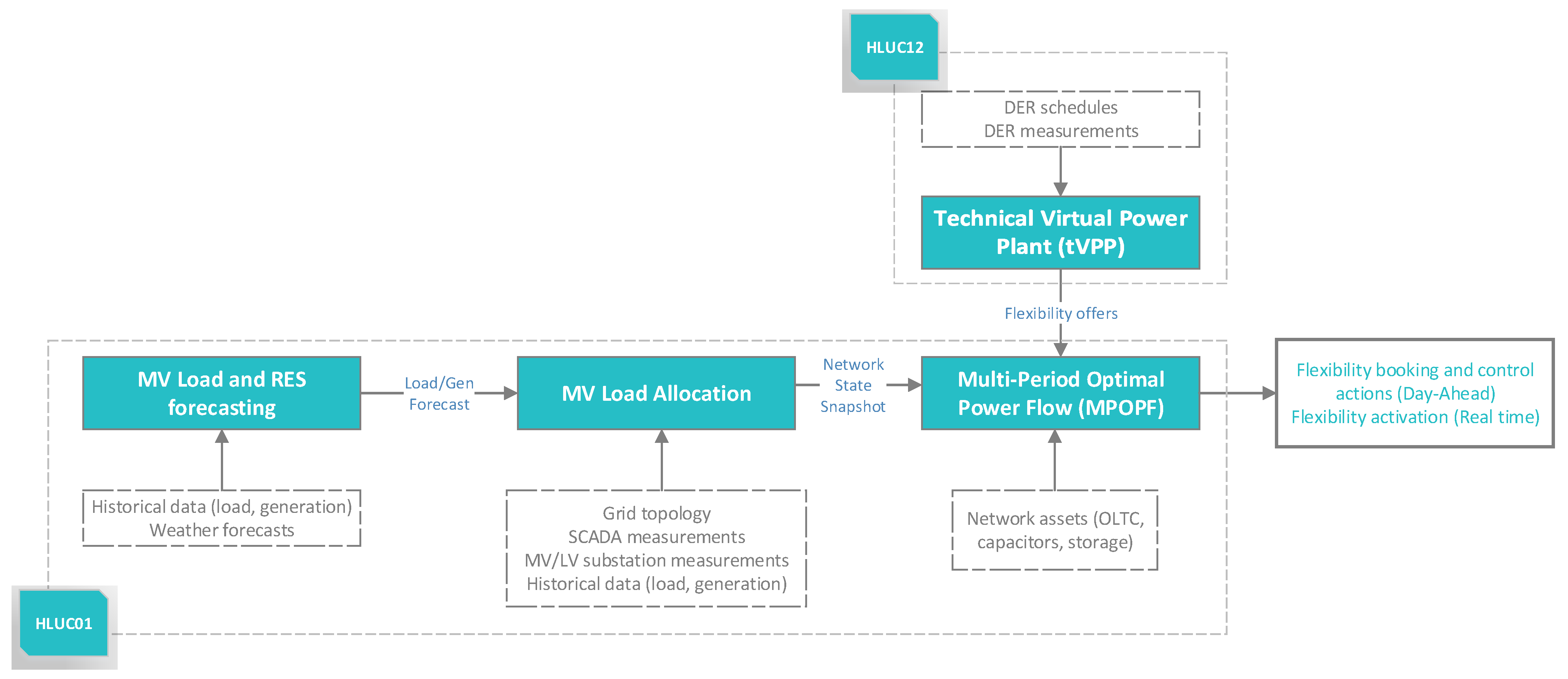
3.1. Cluster 01: Flexibility Management for Optimized MV Network Operation
3.1.1. Description of the Cluster
3.1.2. Objectives of the SRA and Scenarios
- Penetration of RES in the network: the amount of RES is increased to create constraint violations in the MV network and to evaluate the potential of the tools to allow higher levels of hosting capacity. The location and the size of the RES are carefully selected to create challenging situations. The goal is not to perform an exhaustive analysis of the hosting capacity but rather to assess how scaling-up the quantity of RES can be handled by the DSO when empowered with adequate operational tools to manage flexibility;
- Available flexibility of the tVPP: the amount of flexibility is increased compared to the current baseline (i.e., minimal amount of flexibility) to observe how flexibility can be used as an alternative to more traditional solutions such as OLTCs or capacitor banks;
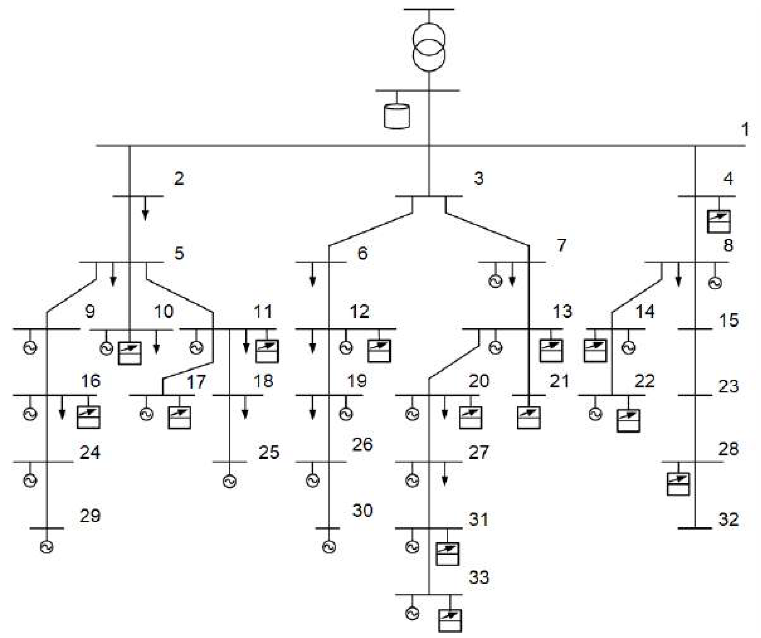
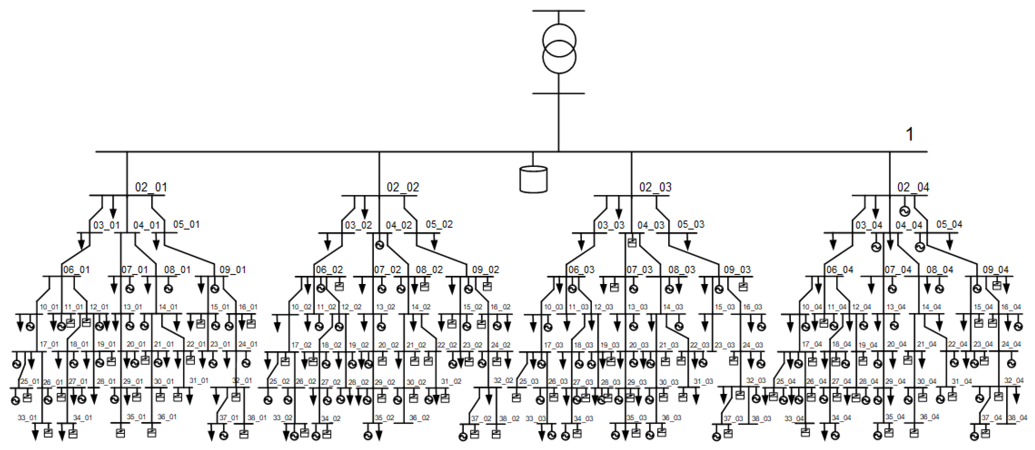
- Network size: the number of nodes is increased as it has a direct influence on the computational effort of the tools (in particular the MPOPF). The network size is relevant for the real-time operation where time constraints are more important than in predictive mode.
- OLTC and capacitor banks control: evaluation of the capability of OLTCs and capacitor banks—usually owned by DSOs—to solve voltage problems by enabling their control through the MPOPF;
- ESS control: integrate ESS to evaluate their impact;
- Reactive power control: as an alternative to local reactive power controls (droop control) used by generators;
- Rural and urban network types: assessment of the performance of the tools under different conditions through the Slovenian and Portuguese network;
- Historical data availability: evaluate the impact on the forecasting accuracy and the MOPF control actions when the length (time-period) of historical data changes;
- Metering primary substation: the grid points for which historical data are available are reduced to evaluate the impact on the MVLA accuracy and MPOPF control actions.
3.1.3. SRA Results
- Baseline—Portugal
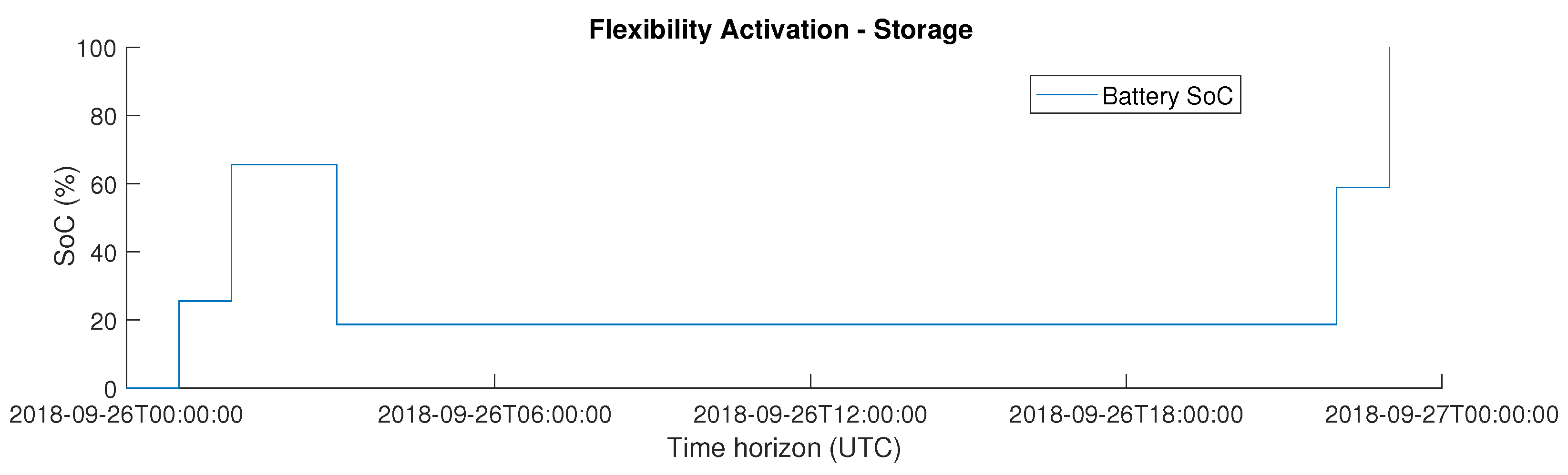
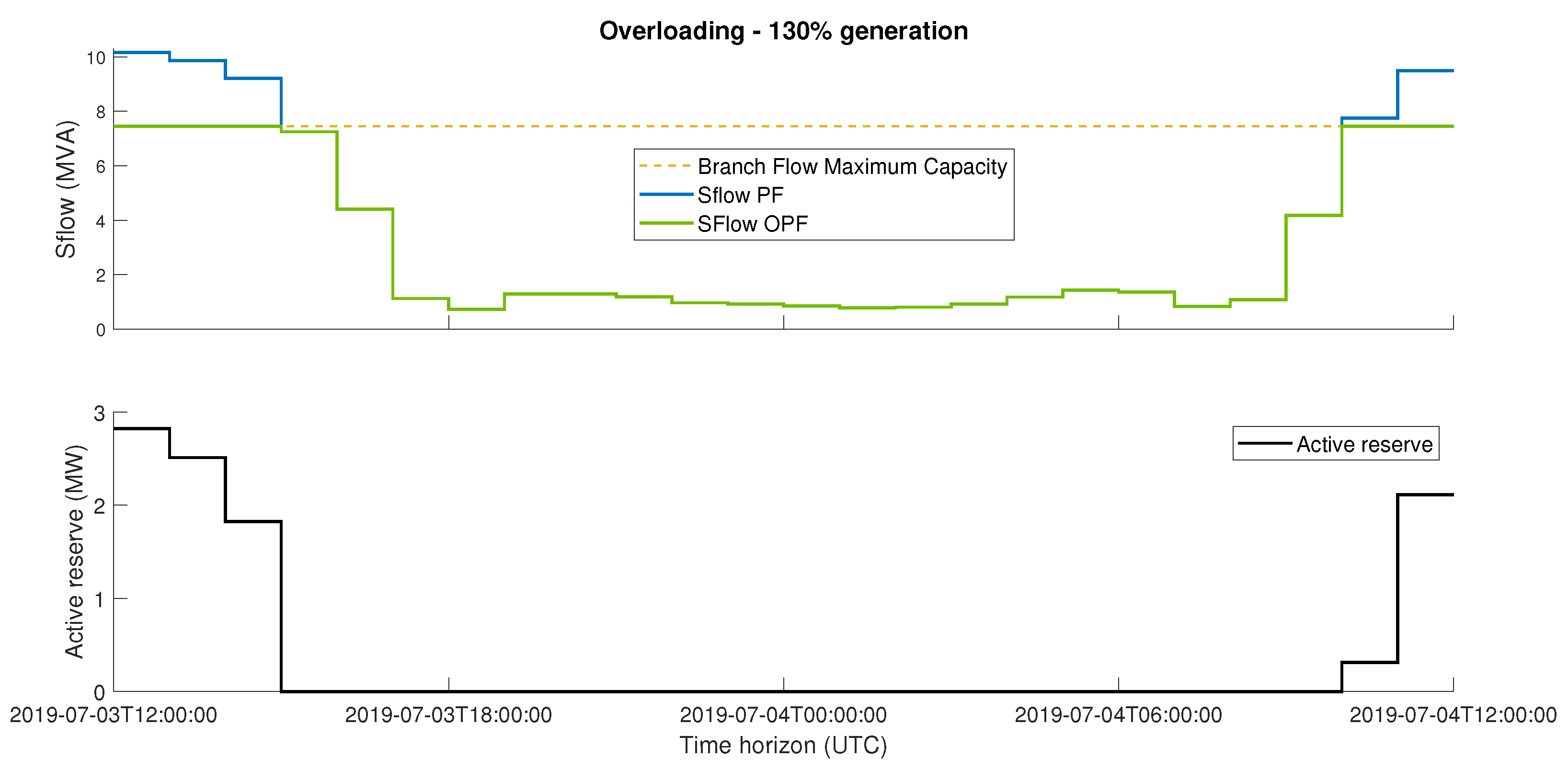
- Overloading Scenario—Portugal
- Baseline—Slovenia
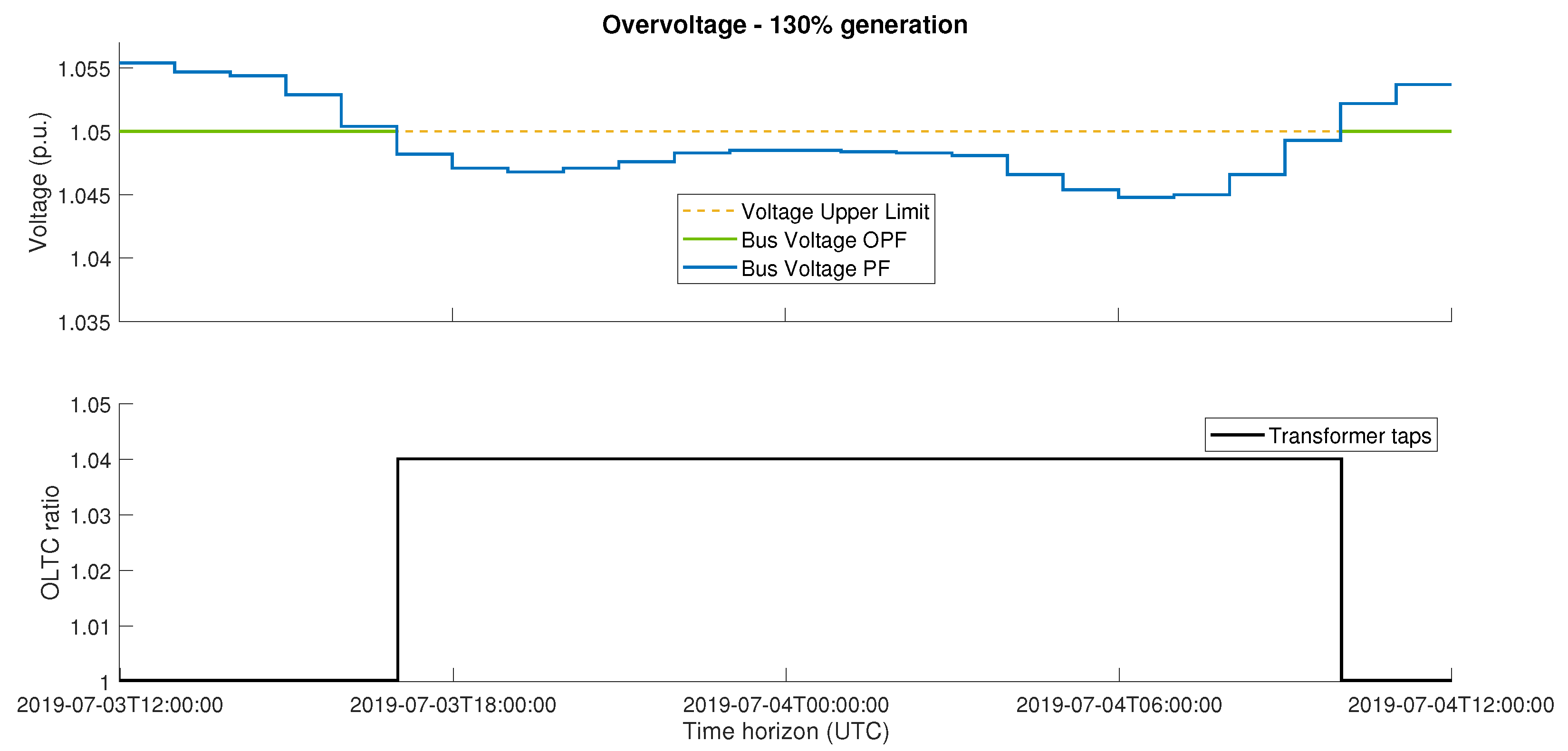
- Slovenia—Overloading and Overvoltage Scenarios
- Network Size Increase—Slovenia
- Limited Historical Data Available—Slovenia
- Limited Measurements Available—Slovenia
3.1.4. Discussion
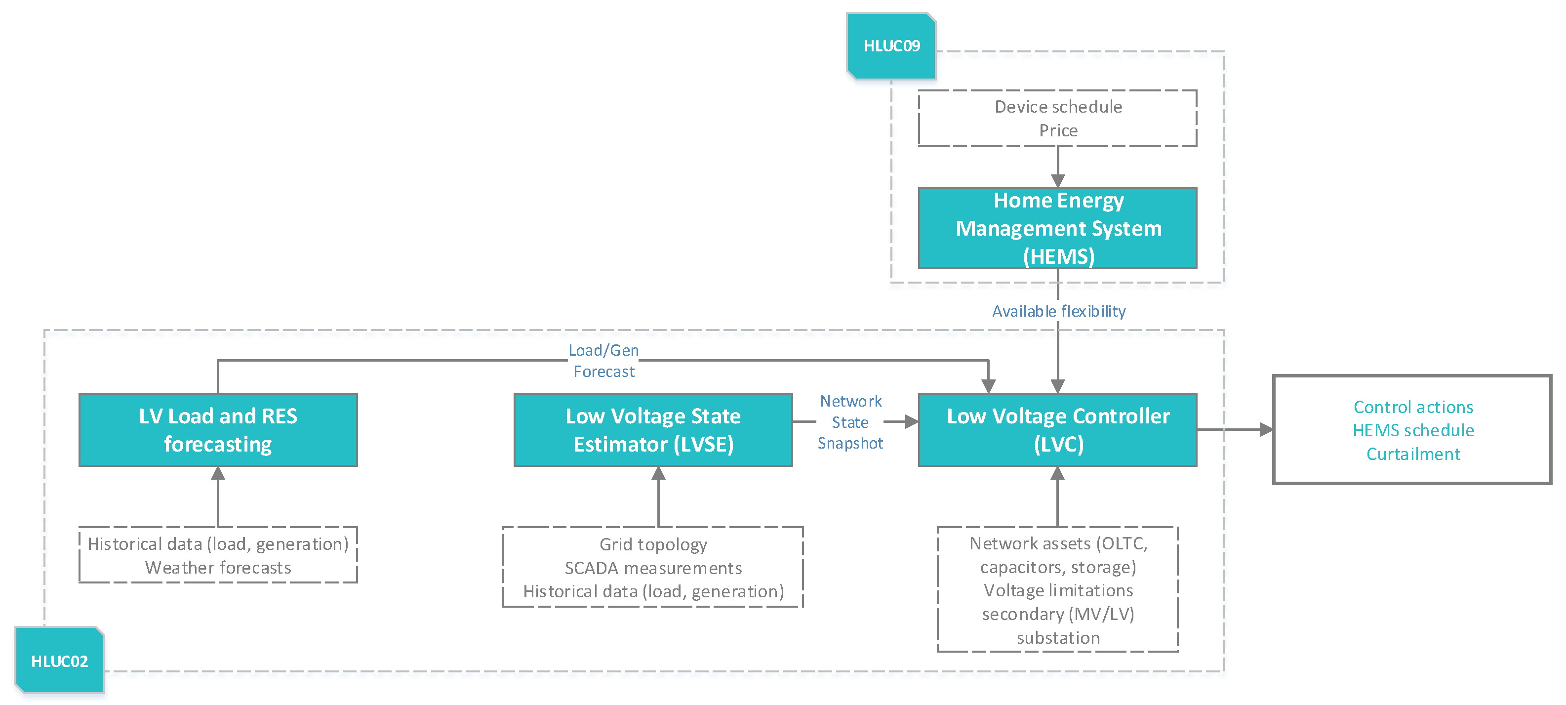
3.2. Cluster 02: Flexibility Management for Optimized LV Network Operation
3.2.1. Description of the Cluster
3.2.2. Objectives of the SRA and Scenarios
- Network size: increase in the number of nodes since it directly influences the computational effort;
- Penetration of RES in the network: increase in the RES penetration in order to create constraints within the LV network and to evaluate the potential of the tool to host more renewable energy;
- Flexibility from HEMS: increase the number of consumers equipped with HEMS to observe whether HEMS can be used as an alternative to DSO’s owned assets such as OLTCs or ESSs;
- Number of controllable devices: increase in the number of controllable devices in the households to evaluate the impact on the resulting load profile and their energy savings.
- OLTC control: evaluate the potential of the set of tools when the secondary substation transformer is controllable, as currently not many secondry substations are equipped with OLTCs;
- Energy storage system control: evaluate the possibility of using central or distributed ESS;
- X/R ratio: modify the the X/R ratio to evaluate the performance of the set of tools in more inductive networks;
- Availability of historical data: modify the amount (time horizon) and the quality of the historical data available for the forecasting and LVSE tools, to assess the impact on the overall forecasting accuracy.
- All controllable resources: the DSO using the LVC considers for operation all available resources, the OLTC, ESS, HEMS, and curtailable microgenerators and loads;
- HEMS: the DSO using the LVC considers for operation the flexibility provided by the HEMS;
- ESS and HEMS: the DSO using the LVC considers for operation the combination of a central ESS (at the secondary of the MV/LV substation) and the flexibility provided by the HEMS;
- Curtailable load and microgeneration: the DSO using the LVC considers for operation the curtailment of the loads and microgenerators.
3.2.3. SRA Results
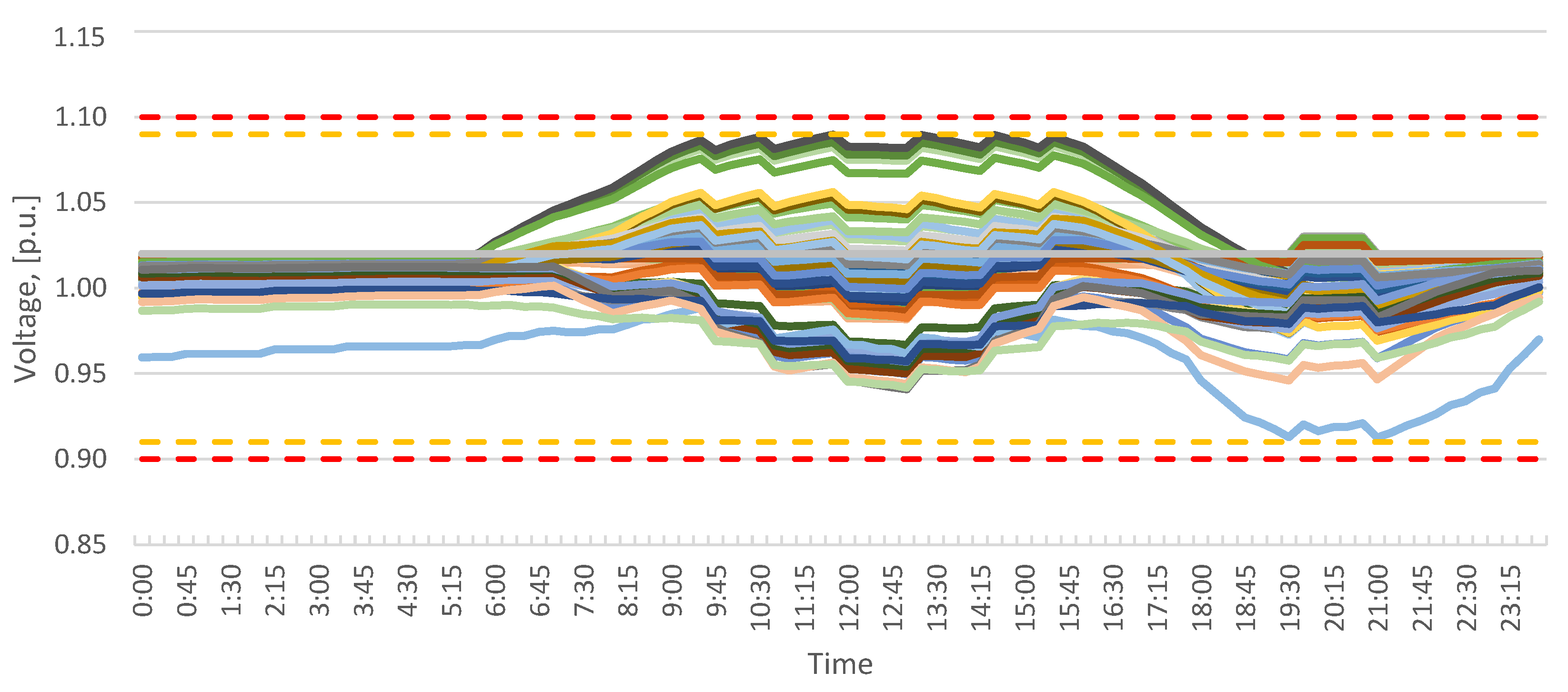
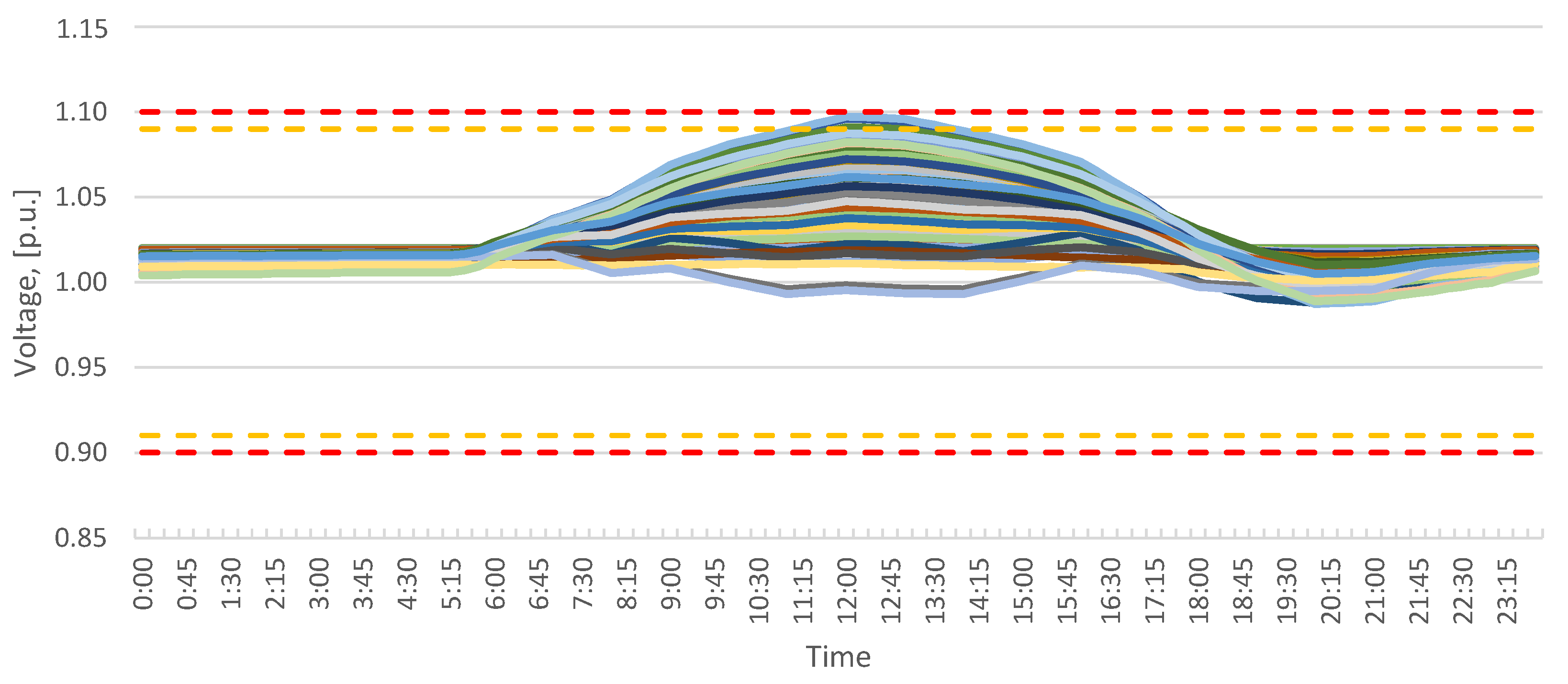
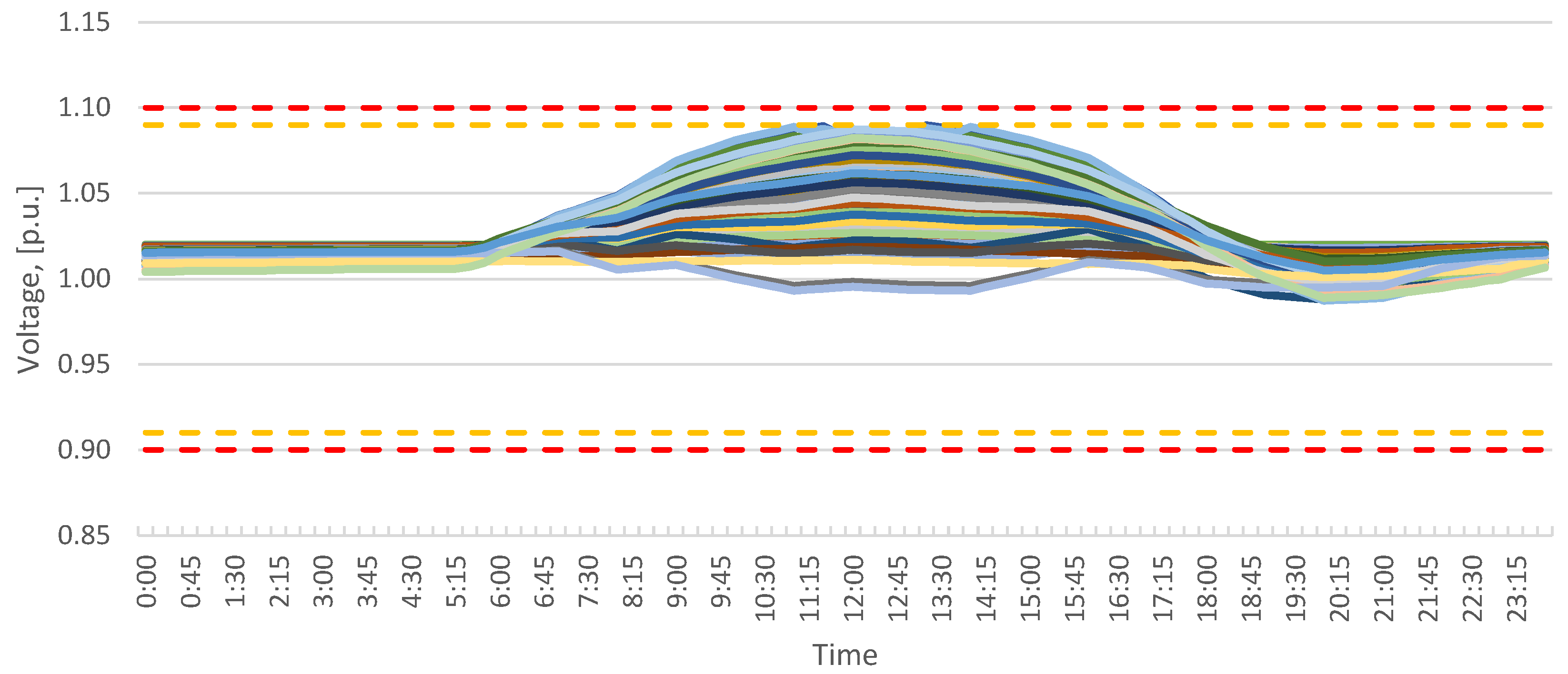
- Baseline—Portugal
- Large Network
- Location of HEMS
- Distributed Energy Storage Systems
- Inductive Network
- Forecast Functions
- Scenario A: 12 months of historical data;
- Scenario B: 3 months of historical data;
- Scenario C: 12 months of historical data, with missing values.
- State Estimation Functions
- Scenario 1 (oracle): real data is considered (all smart meter measurements available);
- Scenario 2: 50% of real-time smart meter measurements available;
- Scenario 3: minimum real-time smart meter measurements available.
3.2.4. Discussion
4. Case Study: SRA for Slovenia
4.1. Cluster 03: Large Customer cVPP
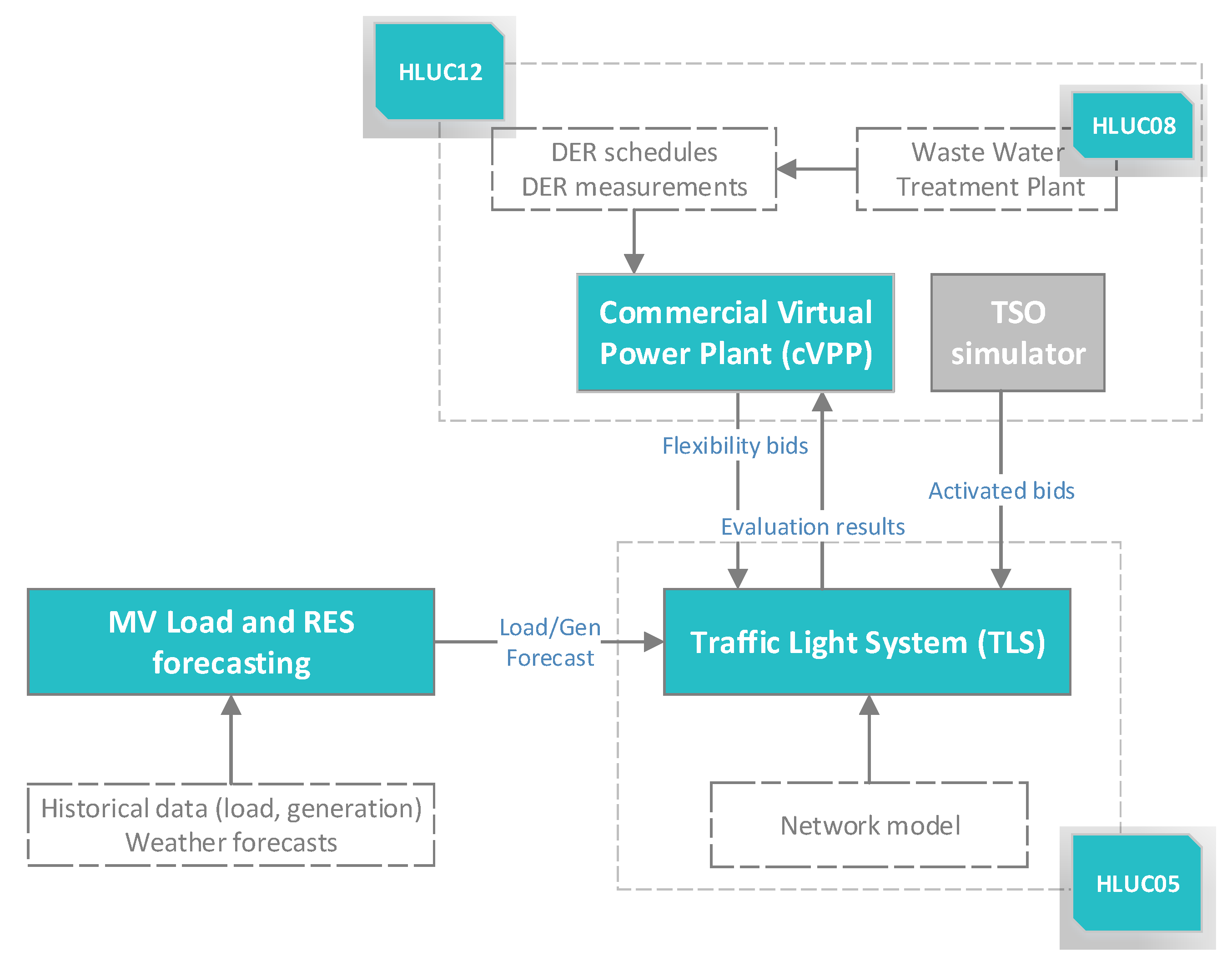
4.1.1. Description of the Cluster
- Day-ahead: In the day-ahead mode, the flexibility operator (FO) periodically sends its flexibility bid offers to the TLS before the gate closure of the market. The TLS analyses these offers and flexibilities, which could lead to network constraints. With this information, the FO can adapt its bids to not interfere with the safe operation of the DSO’s network. Before gate closure, the FO sends its final bids to the TSO, which the TLS has validated. If the TSO accepts the offers, the bids can be activated on the next day for the mFRR market;
- Intraday: In intraday, the TSO can activate the bids accepted on the day before. Thereby, the TSO forwards a bid activation to the TLS. It evaluates the bids to be activated and suggests an alternative bid activation to the FO if the activation would lead to network constraints.
4.1.2. Objectives of the SRA and Scenarios
- What is the maximum flexibility volume in the network which can be activated without violating any network constraints?
- Does the TLS limit the provision of flexibilities in the DSO’s network, and does it curtail the flexibilities fairly?
- Which prerequisites and conditions are needed such that an operation of the TLS is needed?
- Flexibility from the cVPP: increase in the flexibility offered by the cVPP to evaluate the maximum amount of flexibility that each feeder can sustain;
- Network size: the size of the network has a direct influence on the computation time of the TLS. Hence the number of nodes is changed.
- Bid prices: use different bid prices from homogeneous price to increasing and decreasing linear prices;
- Distributed generation: increase in distributed generation in a selection of feeders to evaluate the impact in the amount of upward reserve which could be provided;
- Electric vehicles: addition of electric vehicles in a selection of feeders to evaluate impact in the the amount of upward reserve which could be provided;
- Urban/rural networks: the analysis is carried-out on different grids to be as representative as possible;
- Forecasting accuracy: the impact of the forecasting accuracy on the post-activation evaluation is considered.
4.1.3. SRA Results
- Baseline—Slovenia
- Large Homogeneous Flexibility
- Reduced Homogeneous Flexibility
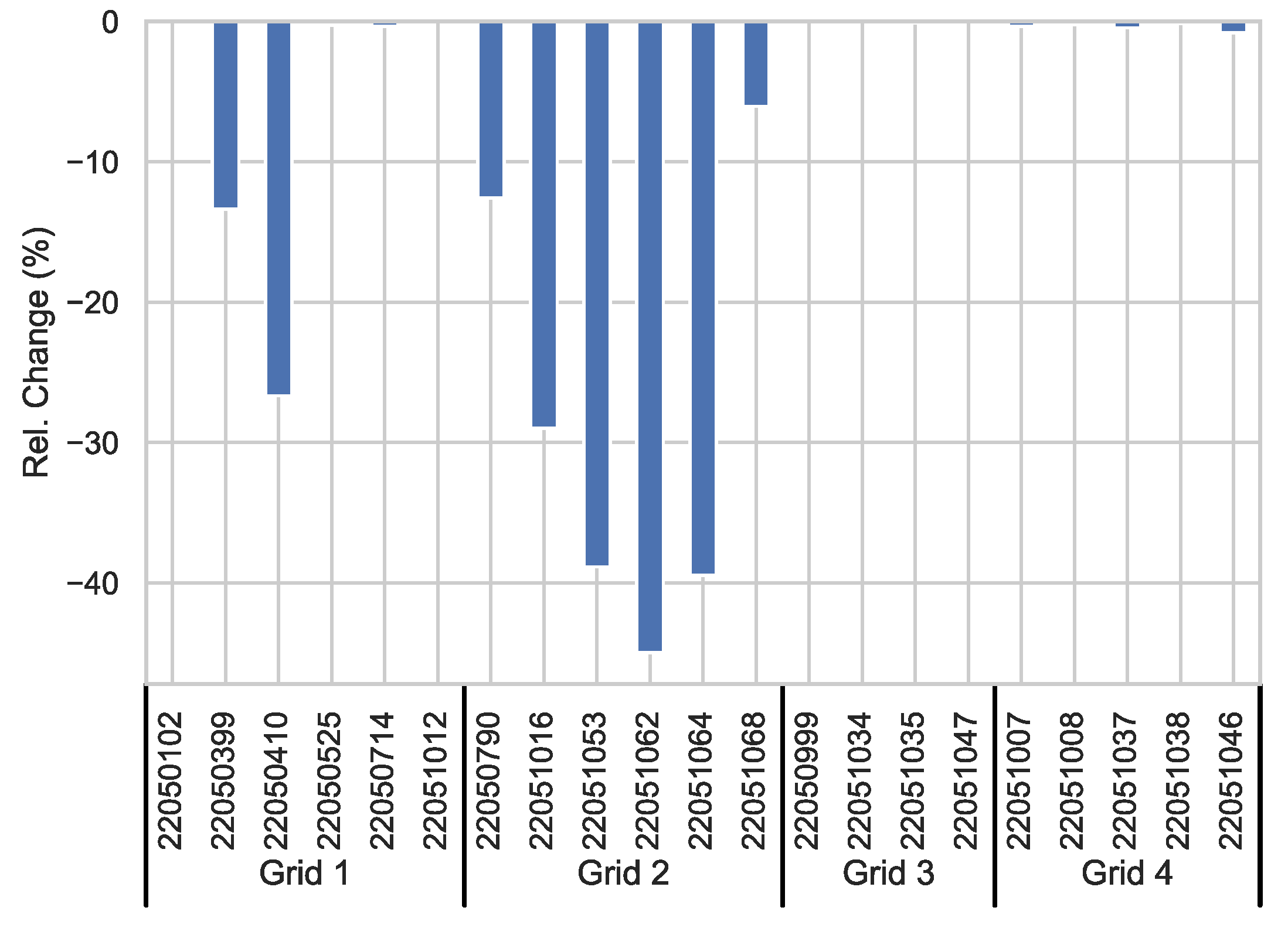
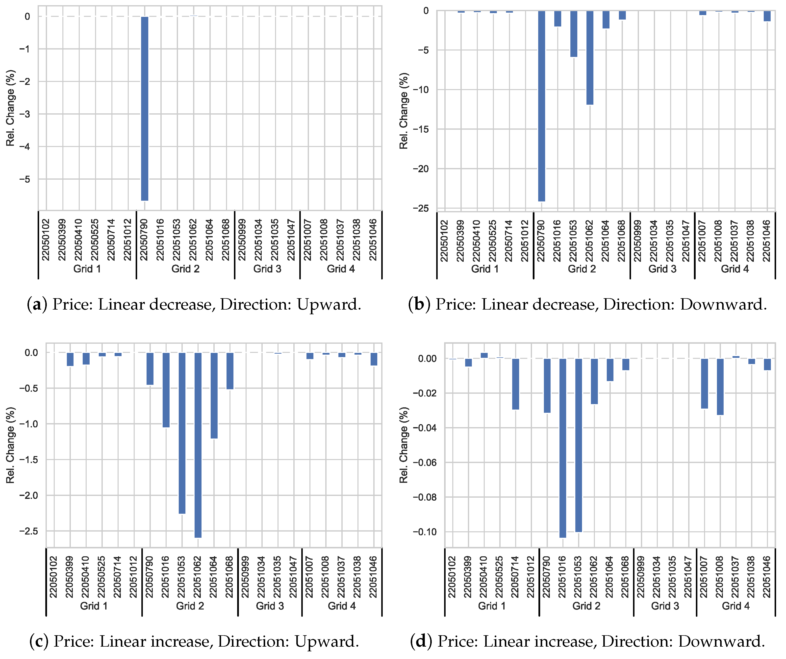
- Linear Prices
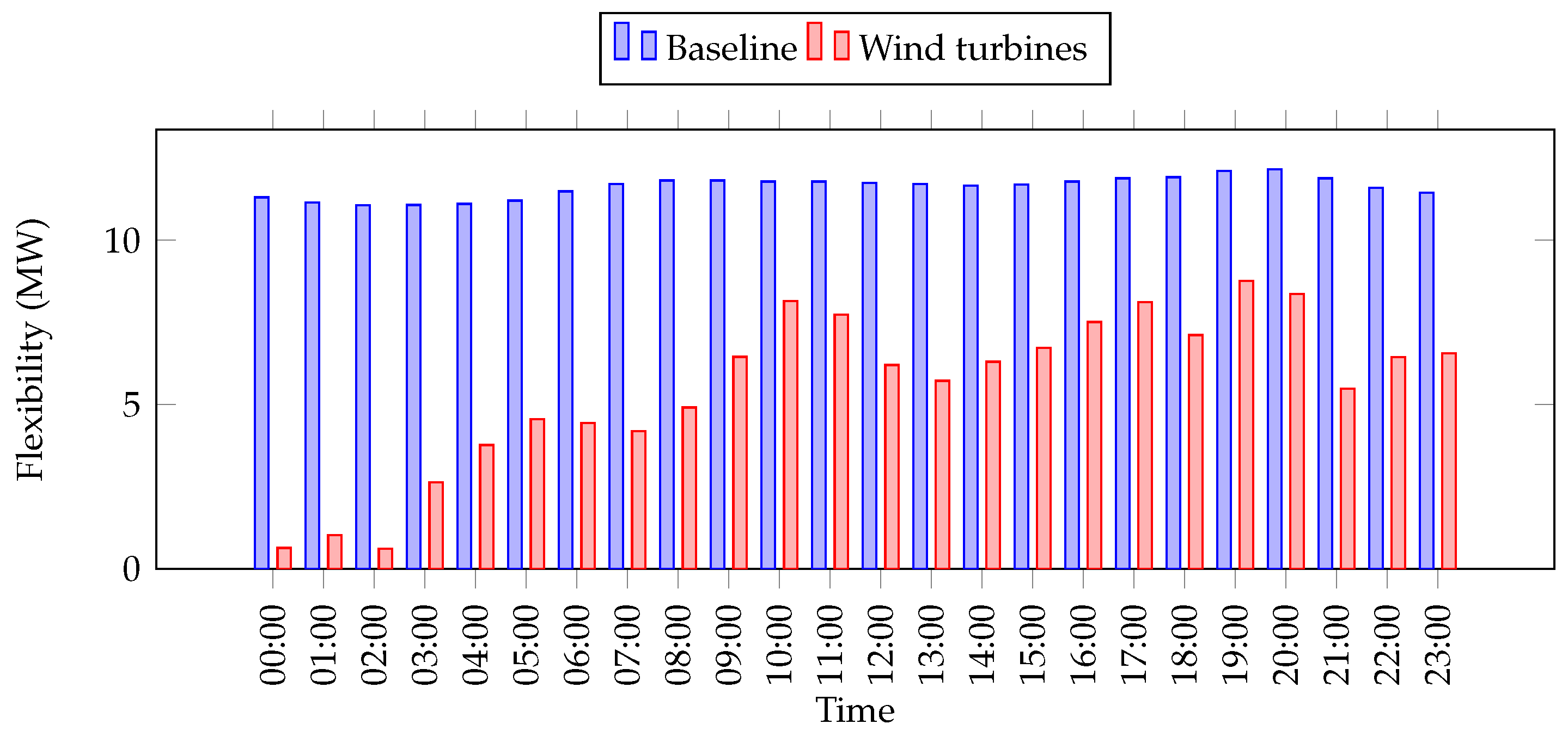
- RES Integration
4.1.4. Discussion
5. Potential Replication Paths
6. Conclusions and Outlook
Author Contributions
Funding
Institutional Review Board Statement
Informed Consent Statement
Data Availability Statement
Acknowledgments
Conflicts of Interest
Abbreviations
| AMI | Advanced Metering Infrastructure |
| BMS | Building Management System |
| cVPP | Commercial Virtual Power Plant |
| DER | Distributed Energy Resources |
| DSM | Demand Side Management |
| DSO | Distribution System Operator |
| ESS | Electric Storage System |
| EV | Electric Vehicles |
| FO | Flexibility Operator |
| GLPK | GNU Linear Programming Kit |
| gm-hub | Grid and Market Hub |
| HEMS | Home Energy Management System |
| HLUC | High Level Use Case |
| HVAC | Heating and Ventilation Air Conditioning |
| ICT | Information and Communication Technology |
| KPI | Key Performance Indicator |
| LVC | Low Voltage Controller |
| LVSE | Low Voltage State Estimator |
| MOPF | Multi Period Optimal Power Flow |
| MVLA | Medium Voltage Load Allocator |
| MW | Mega Watt |
| OLTC | On Load Tap Changer |
| P.U. | Per Unit |
| PV | Photovoltaic |
| RES | Renewable Energy Source |
| REST | Representational State Transfer |
| SCADA | Supervisory Control And Data Acquisition |
| SGAM | Smart Grid Architecture Model |
| SI | Slovenia |
| SRA | Scalability and Replicability Analysis |
| TLS | Traffic Light System |
| tVPP | Technical Virtual Power Pant |
| VPP | Virtual Power Plant |
Appendix A. Developing Environments of InteGrid Tools

| Tool | Prog. lang. | Technologies |
|---|---|---|
| MVLA | C++ | RabbitMQ, Cassandra |
| Load/RES forecasting | Python | RabbitMQ, Cassandra, netCDF4, siphon, scikit-learn, tensorflow, statsmodels, Cron |
| MOPF | C++ | RabbitMQ, Cassandra, Flask, pugixml, ATL |
| LVC | C++ | Cassandra, libcurl, RapidJSON |
| LVSE | C++ | Cassandra, libcurl, RapidJSON |
| TLS | Python | PostgreSQL |
| tVPP/cVPP | Java | RabbitMQ, MongoDB, Kubernetes, MySQL, KumuluzEE, React |
Appendix B. LV Networks Characterization for Cluster 02
Appendix B.1. Baseline
| Line | From | To | Electrical Characteristics | |
|---|---|---|---|---|
| Number | Node | Node | ||
| 1 | 1 | 2 | 0.05666667 | 0.00850000 |
| 2 | 1 | 3 | 0.01904762 | 0.00400000 |
| 3 | 1 | 4 | 0.03666667 | 0.00550000 |
| 4 | 2 | 5 | 0.03095238 | 0.00650000 |
| 5 | 3 | 6 | 0.07692000 | 0.01800000 |
| 6 | 3 | 7 | 0.07000001 | 0.01050000 |
| 7 | 4 | 8 | 0.06666667 | 0.01000000 |
| 8 | 5 | 9 | 0.04666667 | 0.00700000 |
| 9 | 5 | 10 | 0.10395000 | 0.00525000 |
| 10 | 5 | 11 | 0.21874994 | 0.01050000 |
| 11 | 6 | 12 | 0.29166659 | 0.01400000 |
| 12 | 7 | 13 | 0.02333334 | 0.00350000 |
| 13 | 8 | 14 | 0.19890000 | 0.00975000 |
| 14 | 8 | 15 | 0.12415000 | 0.00975000 |
| 15 | 9 | 16 | 0.02333334 | 0.00350000 |
| 16 | 11 | 17 | 0.24955000 | 0.00525000 |
| 17 | 11 | 18 | 0.09550000 | 0.00750000 |
| 18 | 12 | 19 | 0.03809523 | 0.00800000 |
| 19 | 13 | 20 | 0.15280000 | 0.01200000 |
| 20 | 13 | 21 | 0.48405000 | 0.01575000 |
| 21 | 14 | 22 | 1.21210000 | 0.02550000 |
| 22 | 15 | 23 | 0.26740000 | 0.02100000 |
| 23 | 16 | 24 | 0.04666667 | 0.00350000 |
| 24 | 18 | 25 | 0.16135000 | 0.00525000 |
| 25 | 19 | 26 | 0.02380952 | 0.00500000 |
| 26 | 20 | 27 | 0.18749995 | 0.00900000 |
| 27 | 23 | 28 | 0.93450000 | 0.02100000 |
| 28 | 24 | 29 | 0.18440000 | 0.00600000 |
| 29 | 26 | 30 | 0.05333334 | 0.00400000 |
| 30 | 27 | 31 | 0.21420000 | 0.01050000 |
| 31 | 28 | 32 | 0.32270000 | 0.01050000 |
| 32 | 31 | 33 | 0.16135000 | 0.00525000 |
| Installed Capacity | |||||||||
|---|---|---|---|---|---|---|---|---|---|
| Loads, [kVA] | Generators, [kVA] | HEMS, [kVA] | |||||||
| Node | Phase R | Phase S | Phase T | Phase R | Phase S | Phase T | Phase R | Phase S | Phase T |
| 2 | 3.45 | 3.45 | - | - | - | - | - | - | - |
| 4 | - | - | - | - | - | - | - | 5.75 | - |
| 5 | - | - | 3.45 | - | - | - | - | - | - |
| 6 | 1.15 | - | - | - | - | - | - | - | - |
| 7 | 6.90 | - | - | 5.75 | - | - | - | - | - |
| 8 | 3.45 | 3.45 | 3.45 | 5.75 | - | - | - | - | - |
| 9 | - | - | - | 3.45 | - | - | - | - | - |
| 10 | 3.45 | 6.90 | - | - | 5.75 | - | - | 5.75 | - |
| 11 | 3.45 | - | - | - | - | 3.45 | - | - | 5.75 |
| 12 | 3.45 | 3.45 | - | - | - | 3.45 | 5.75 | - | 5.75 |
| 13 | - | - | - | 3.45 | - | - | 5.75 | - | - |
| 14 | - | - | - | 5.75 | - | - | 5.75 | - | - |
| 16 | - | 6.90 | - | - | 3.45 | - | 5.75 | 5.75 | 5.75 |
| 17 | - | - | - | - | - | - | 5.75 | - | - |
| 18 | - | 3.45 | 3.45 | - | - | - | - | - | - |
| 19 | 3.45 | 3.45 | - | - | - | 5.75 | - | - | - |
| 20 | - | 3.45 | 3.45 | 5.75 | - | - | 6.90 | 5.75 | - |
| 21 | - | - | - | - | - | - | - | 5.75 | 5.75 |
| 22 | - | - | - | 1.15 | - | - | - | 3.45 | 3.45 |
| 24 | - | - | - | 5.75 | 5.75 | 5.75 | - | - | - |
| 25 | - | - | - | - | - | 5.75 | - | - | - |
| 26 | - | - | - | - | 5.75 | 3.45 | - | - | - |
| 27 | 6.90 | 3.45 | 3.45 | 3.45 | - | - | - | - | - |
| 28 | - | - | - | - | - | - | - | 3.45 | - |
| 29 | - | - | - | - | - | 5.75 | - | - | - |
| 30 | - | - | - | - | - | 5.75 | - | - | - |
| 31 | - | - | - | 3.45 | 3.45 | - | - | 6.90 | - |
| 33 | - | - | - | 1.15 | - | - | - | - | 5.75 |
Appendix B.2. Large Network
Appendix B.3. HEMS Location
| Installed Capacity | |||||||||
|---|---|---|---|---|---|---|---|---|---|
| Loads, [kVA] | Generators, [kVA] | HEMS, [kVA] | |||||||
| Node | Phase R | Phase S | Phase T | Phase R | Phase S | Phase T | Phase R | Phase S | Phase T |
| 2 | 3.45 | - | - | - | - | - | - | - | - |
| 5 | - | 3.45 | - | - | - | - | - | - | - |
| 6 | - | - | 3.45 | - | - | - | - | - | - |
| 7 | 6.90 | - | - | 5.75 | - | - | - | - | - |
| 8 | 3.45 | 3.45 | 3.45 | 5.75 | - | - | - | - | - |
| 9 | 6.90 | 3.45 | 3.45 | 3.45 | - | - | - | - | - |
| 10 | 3.45 | 6.90 | - | - | 5.75 | - | - | - | - |
| 11 | 3.45 | - | - | - | - | 3.45 | - | - | - |
| 12 | 3.45 | 3.45 | - | - | - | 3.45 | - | - | - |
| 13 | 6.90 | 3.45 | 3.45 | 3.45 | - | - | - | - | - |
| 14 | - | - | - | 5.75 | - | - | - | - | - |
| 16 | - | 6.90 | - | - | 3.45 | - | - | - | - |
| 17 | - | - | - | 5.75 | - | - | 5.75 | - | - |
| 18 | - | 3.45 | 3.45 | - | - | - | - | - | - |
| 19 | 3.45 | 3.45 | - | - | - | 5.75 | - | - | - |
| 20 | - | 3.45 | 3.45 | 5.75 | - | - | - | - | - |
| 22 | - | - | - | 1.15 | - | - | 6.90 | 3.45 | 3.45 |
| 23 | 3.45 | - | - | - | - | - | - | - | - |
| 24 | - | - | - | 5.75 | 5.75 | 5.75 | 5.75 | 5.75 | 5.75 |
| 25 | - | - | - | - | - | 5.75 | - | 5.75 | 5.75 |
| 26 | - | - | - | - | 5.75 | 3.45 | - | 5.75 | - |
| 27 | 6.90 | 3.45 | 3.45 | 3.45 | - | - | - | - | - |
| 29 | - | - | - | - | - | 5.75 | 5.75 | 5.75 | 5.75 |
| 30 | - | - | - | - | - | 5.75 | - | - | 6.90 |
| 31 | - | - | - | 3.45 | 3.45 | - | - | 6.90 | - |
| 32 | - | - | - | - | - | - | - | 3.45 | 3.45 |
| 33 | - | - | 3.45 | 1.15 | - | - | 3.45 | - | - |
Appendix B.4. Inductive Network
| Line | From | To | Electrical Characteristics | |
|---|---|---|---|---|
| Number | Node | Node | ||
| 1 | 1 | 2 | 0.04006939 | 0.01202082 |
| 2 | 1 | 3 | 0.01346870 | 0.00565685 |
| 3 | 1 | 4 | 0.02592725 | 0.00777817 |
| 4 | 2 | 5 | 0.02188664 | 0.00919239 |
| 5 | 3 | 6 | 0.05439065 | 0.02545584 |
| 6 | 3 | 7 | 0.04949748 | 0.01484924 |
| 7 | 4 | 8 | 0.04714045 | 0.01414214 |
| 8 | 5 | 9 | 0.03299832 | 0.00989949 |
| 9 | 5 | 10 | 0.07350375 | 0.00742462 |
| 10 | 5 | 11 | 0.15467957 | 0.01484924 |
| 11 | 6 | 12 | 0.20623942 | 0.01979899 |
| 12 | 7 | 13 | 0.01649916 | 0.00494975 |
| 13 | 8 | 14 | 0.14064354 | 0.01378858 |
| 14 | 8 | 15 | 0.08778731 | 0.01378858 |
| 15 | 9 | 16 | 0.01649916 | 0.00494975 |
| 16 | 11 | 17 | 0.17645850 | 0.00742462 |
| 17 | 11 | 18 | 0.06752870 | 0.01060660 |
| 18 | 12 | 19 | 0.02693740 | 0.01131371 |
| 19 | 13 | 20 | 0.10804592 | 0.01697056 |
| 20 | 13 | 21 | 0.34227504 | 0.02227386 |
| 21 | 14 | 22 | 0.85708413 | 0.03606245 |
| 22 | 15 | 23 | 0.18908035 | 0.02969848 |
| 23 | 16 | 24 | 0.03299832 | 0.00494975 |
| 24 | 18 | 25 | 0.11409168 | 0.00742462 |
| 25 | 19 | 26 | 0.01683587 | 0.00707107 |
| 26 | 20 | 27 | 0.13258249 | 0.01272792 |
| 27 | 23 | 28 | 0.66079129 | 0.02969848 |
| 28 | 24 | 29 | 0.13039049 | 0.00848528 |
| 29 | 26 | 30 | 0.03771237 | 0.00565685 |
| 30 | 27 | 31 | 0.15146227 | 0.01484924 |
| 31 | 28 | 32 | 0.22818336 | 0.01484924 |
| 32 | 31 | 33 | 0.11409168 | 0.00742462 |
References
- Pérez-Arriagaa, I.; Knittel, C.; Bharatkumar, A.; Luke, M.; Birk, M.; Miller, R.; Burger, S. MIT Energy Initiative: Utility of the Future. In Technical Report; MIT: Cambridge, MA, USA, 2016. [Google Scholar]
- Alotaibi, I.; Abido, M.A.; Khalid, M.; Savkin, A.V. A Comprehensive Review of Recent Advances in Smart Grids: A Sustainable Future with Renewable Energy Resources. Energies 2020, 13, 6269. [Google Scholar] [CrossRef]
- Boscán, L.; Poudineh, R. Chapter 19—Business Models for Power System Flexibility: New Actors, New Roles, New Rules. In Future of Utilities Utilities of the Future; Sioshansi, F.P., Ed.; Academic Press: Boston, UK, 2016; pp. 363–382. [Google Scholar] [CrossRef]
- Zhang, Y.; Chen, W.; Gao, W. A survey on the development status and challenges of smart grids in main driver countries. Renew. Sustain. Energy Rev. 2017, 79, 137–147. [Google Scholar] [CrossRef]
- Flavia, S.; Julija, V.; COVRIG; Catalin-Felix; Maria, M.A.; Gianluca, F. Smart grid projects outlook 2017: Facts, figures and trends in Europe. In Technical Report; Joint Research Center (JRC): Ispra, Italy, 2017. [Google Scholar]
- Prettico, G.; Flammini, M.; Andreadou, N.; Vitiello, S.; Fulli, G.; Masera, M. Distribution System Operators Observatory 2018. In Technical Report JRC113926; Joint Research Center (JRC): Ispra, Italy, 2019. [Google Scholar]
- H2020 Project InteGrid. Available online: https://integrid-h2020.eu/ (accessed on 19 November 2020).
- Rivero, E.; Sebastian-Viana, M.; Ulian, A.; Stromsather, J. The evolvDSO project: Key services for the evolution of DSOs roles. In Proceedings of the CIRED Lyon 2015 Workshop, Lyon, France, 15–18 June 2015. [Google Scholar]
- FP7 Project evolvDSO. Available online: https://www.edsoforsmartgrids.eu/projects/edso-projects/evolvdso/ (accessed on 19 November 2020).
- FP7 Project Grid+. Available online: https://www.edsoforsmartgrids.eu/projects/edso-projects/past-projects/grid/ (accessed on 19 November 2020).
- Sigrist, L.; May, K.; Morch, A.; Verboven, P.; Vingerhoets, P.; Rouco, L. On Scalability and Replicability of Smart Grid Projects—A Case Study. Energies 2016, 9, 195. [Google Scholar] [CrossRef] [Green Version]
- FP7 Project Grid4EU. Available online: https://ses.jrc.ec.europa.eu/grid4eu (accessed on 19 November 2020).
- FP7 Project IGREENGRID. Available online: https://cordis.europa.eu/project/id/308864 (accessed on 19 November 2020).
- H2020 Project InterFlex. Available online: https://interflex-h2020.com/ (accessed on 19 November 2020).
- Cen(2012). CEN-CENELEC-ETSI Smart Grid Coordination Group. Smart Grid Reference Architecture. Available online: https://www.cencenelec.eu/standards/Sectorsold/SustainableEnergy/SmartGrids/Pages/default.aspx (accessed on 19 November 2020).
- Uslar, M.; Rohjans, S.; Neureiter, C.; Pröstl Andrén, F.; Velasquez, J.; Steinbrink, C.; Efthymiou, V.; Migliavacca, G.; Horsmanheimo, S.; Brunner, H.; et al. Applying the Smart Grid Architecture Model for Designing and Validating System-of-Systems in the Power and Energy Domain: A European Perspective. Energies 2019, 12, 258. [Google Scholar] [CrossRef] [Green Version]
- Pinto, R.; Bessa, R.J.; Matos, M.A. Multi-period flexibility forecast for low voltage prosumers. Energy 2017, 141, 2251–2263. [Google Scholar] [CrossRef] [Green Version]
- André, R.; Lopes, D.; Fonseca, D.; Almeida, B.; Bessa, R.J.; Madureira, A.; Simões, M.; Silva, J.; Sampaio, G.; Andrade, J.; et al. InteGrid pilot in Portugal: Smart grid based flexibility management tools for LV and MV predictive grid operation. In Proceedings of the CIRED Berlin 2020 Workshop, Berlin, Germany, 22–23 September 2020. [Google Scholar]
- Lopes, D.; André, R.; Moreira, J.; Simões, M.; Sampaio, G.; Rua, D.; Machado, P.; Bessa, R.J.; Abreu, C.; Madureira, A. From home energy management system local flexibility to low-voltage predictive grid management. In Proceedings of the CIRED 2020 Workshop, Virtual, Berlin, Germany, 22–23 September 2020. [Google Scholar]
- Nilsson, A.; Wester, M.; Lazarevic, D.; Brandt, N. Smart homes, home energy management systems and real-time feedback: Lessons for influencing household energy consumption from a Swedish field study. Energy Build. 2018, 179, 15–25. [Google Scholar] [CrossRef]
- Ursula, K.; Boris, T. Demonstration of the technical and commercial VPP concept: Slovenian demo in the InteGrid project. In Proceedings of the CIRED 2018 Workshop, Ljubljana, Slovenia, 7–8 June 2018. [Google Scholar]
- Leimgruber, J.L.B.F.; Korner, C.; Gutschi, C. The Traffic Light System to support Flexibility Exploitation from stressed distribution grids. In Proceedings of the CIRED 2019 Madrid, Virtual, Madrid, Spain, 3–6 June 2019. [Google Scholar]
- Bessa, R.; Coelho, F.; Rodrigues, X.; Alonso, A.; Soares, T.; Pires, G.; Matos, P.; Prates, I.; Shahrokni, H.; Mäkivierikko, A. Grid and Market Hub: Empowering Local Energy Communities in InteGrid. In Proceedings of the CIRED 2018 Workshop, Ljubljana, Slovenia, 7–8 June 2018. [Google Scholar]
- Moreira, J.; Bernardo, R.; Prata, R.; Krisper, U.; Bessa, R.J.; Coelho, F.; Schwarzländer, F. Service catalyst providing a neutral framework for supporting grid operation, while promoting market-based services: Grid and market hub. In Proceedings of the CIRED 2020 Workshop, Virtual, Berlin, Germany, 22–23 September 2020. [Google Scholar]
- U.S department of Energy. The Smart Grid, What Makes a Grid “Smart?”. Available online: https://www.smartgrid.gov/the_smart_grid/smart_grid.html (accessed on 19 November 2020).
- Edris, A.A.; D’Andrade, B.W. 2—Transmission Grid Smart Technologies. In The Power Grid; D’Andrade, B.W., Ed.; Academic Press: Cambridge, MA, USA, 2017; pp. 37–55. [Google Scholar] [CrossRef]
- Bessa, R.J. Use Cases and Requirements. In Technical Report D1.2, H2020 InteGrid Project; Publisher Integrid: Lisboa, Portugal, 2017. [Google Scholar]
- Baut, J.L.; Potenciano-Menci, S.; Herndler, B.; Korner, C.; Rao, B.; Henein, S.; Potenciano-Menci, S.; López, G.; Domingo, J. Technical Scalability and Replicability of the InteGrid Smart Grid Functionalities. Technical Report D8.1, H2020 InteGrid Project. 2019. Available online: https://www.mdpi.com/1996-1073/13/15/3818 (accessed on 19 November 2020).
- Cossent, R.; Lind, L.; Correa, M.; Gómez, T.; Pimentel, N.; Baut, J.L.; Menci, S.P.; Bharath-Varsh, R.; Silva, M.; Ávila, J.P.; et al. Economic and regulatory scalability and replicability of the InteGrid smart grid functionalities. In Technical Report D8.2, H2020 InteGrid Project; Publisher Integrid: Lisboa, Portugal, 2020. [Google Scholar]
- Menci, S.P.; Baut, J.L.; Domingo, J.M.; López, G.L.; Arín, R.C.; Silva, M.P. A Novel Methodology for the Scalability Analysis of ICT Systems for Smart Grids Based on SGAM: The InteGrid Project Approach. Energies 2020, 13, 3818. [Google Scholar] [CrossRef]
- Baut, J.; Kadam, S.; Menci, S.; Stefan, M.; Costa, J.M.; Silva, M.; Cossent, R.; Lind, L.; Morgado, M.; Bessa, R.J.; et al. Definition of Scenarios and Methodology for the Scalability and Replicability Analysis. In Technical Report MS9, H2020 InteGrid Project; Publisher Integrid: Lisboa, Portugal, 2017. [Google Scholar]
- Rodríguez Calvo, A. Scalability and Replicability of the Impact of Smart Grid Solutions in Distribution Systems. Ph.D. Thesis, Universidad Pontificia Comillas, Madrid, Spain, 2017. [Google Scholar]
- Viana, J.; Sousa, J.; Bessa, R.J. Load forecasting benchmark for smart meter data. In Proceedings of the 13th IEEE PES PowerTech Conference, Milano, Italy, 23–27 June 2019. [Google Scholar]
- Andrade, J.R.; Bessa, R.J. Improving renewable energy forecasting with a grid of numerical weather predictions. IEEE Trans. Sustain. Energy 2017, 8, 1571–1580. [Google Scholar] [CrossRef] [Green Version]
- Costa, J.; Trocato, C.; Moreira, J.; Rua, D.; Madureira, A.; Fonseca, D. LV Network Control Architecture: H2020 InteGrid Case Study. In Proceedings of the CIRED 2018 Workshop, Ljubljana, Slovenia, 7–8 June 2018. [Google Scholar]
- Simões, M.; Madureira, A.G. Predictive Voltage Control: Empowering Domestic Customers With a Key Role in the Active Management of LV Networks. Appl. Sci. 2020, 10, 2653. [Google Scholar] [CrossRef] [Green Version]
- Abreu, C.; Soares, I.; Oliveira, L.; Rua, D.; Machado, P.; Carvalho, L.; Peças Lopes, J.A. Application of genetic algorithms and the cross-entropy method in practical home energy management systems. IET Renew. Power Gener. 2019, 13, 1474–1483. [Google Scholar] [CrossRef]
- Simões, M.; Sampaio, G.; Madureira, A.; Bessa, R.; Pereira, J.; Lopes, D.; Fonseca, D.; Godinho Matos, P.; Pires, R. Avoid technical problems in LV networks: From data-driven monitoring to predictive control. In Proceedings of the CIRED 2019 Madrid, Virtual, Madrid, Spain, 3–6 June 2019. [Google Scholar]
- Bessa, R.; Sampaio, G.; Miranda, V.; Pereira, J. Probabilistic Low-Voltage State Estimation Using Analog-Search Techniques. In Proceedings of the 2018 Power Systems Computation Conference (PSCC), Dublin, Ireland, 11–15 June 2018. [Google Scholar]
- Ciric, R.M.; Feltrin, A.P.; Ochoa, L.F. Power flow in four-wire distribution networks-general approach. IEEE Trans. Power Syst. 2003, 18, 1283–1290. [Google Scholar] [CrossRef] [Green Version]
- Glover, J.D.; Sarma, M.S.; Overbye, T.J. Power Distribution. In Power Systems Analysis and Design; Thomson: Stanford, CT, USA, 2007. [Google Scholar]


| Scenario Name | Network | Variation |
|---|---|---|
| Baseline Portugal | PT demo | Baseline—No variation considered |
| Overloading occurrence | PT demo | RES connected to create overloading. Different control actions are tested (ESS; tVPP) |
| Baseline Slovenia | SI demo | Baseline—No variation considered |
| Overloading/voltage occurrence | SI demo | RES connected to create overloading and overvoltage. OLTC and the tVPP are available |
| Network size increase | SI demo | Size of the network is increased |
| Limited measurements available | SI demo | Historical data for primary substation transformers only |
| Reduction of Overloading Occurrences (%) | |
|---|---|
| Energy Storage System | 100 |
| tVPP (MV customers) | 100 |
| Reduction of Overloading Occurrences (%) | Reduction of Overvoltage Occurrences (%) | |||
|---|---|---|---|---|
| 10–30% | =40.0% | 10–30% | =40.0% | |
| RES Growth | RES Growth | RES Growth | RES Growth | |
| tVPP(generation curtailment) | 100 | 70 | - | - |
| OLTC | - | - | 100 | 100 |
| Scenario Name | Network | Variation |
|---|---|---|
| Baseline Portugal | Typical PT LV network | Baseline—No variation considered |
| Large network | Typical PT LV network | Increase the number of nodes |
| Location of HEMS | Typical PT LV network | Change the location of the HEMS to primarily at the end of the feeders |
| Distributed ESS | Typical PT LV network | Introduce controllable distributed ESS in the network |
| Inductive network | Typical PT LV network | Modify the networks parameters to resemble an urban network |
| Forecast functions | Typical PT LV network | Variation of the data used to train the algorithms |
| State estimation functions | Typical PT LV network | Real data consideration and variation thereof the smart meter data available |
| Voltage Problem | HEMS Flexibility, | , | Reduction, | |
|---|---|---|---|---|
| Solved? | [kWh] | [kWh] | [%] | |
| Homogeneous Distribution of HEMS (Baseline) | ||||
| HEMS | No | 16.53 | - | 0.09% |
| HEMS and ESS | No | 16.41 | 94.63 | 0.11% |
| HEMS located at the end of the feeders | ||||
| HEMS | Yes | 4.42 | - | 0.14% |
| HEMS and ESS | Yes | 4.32 | 44.13 | 0.01% |
| Node | ESS Characteristics | |
|---|---|---|
| Power, [kW] | Capacity, [kWh] | |
| 1 | 50.00 | 100.00 |
| 18 | 10.00 | 20.00 |
| 23 | 10.00 | 20.00 |
| 24 | 10.00 | 20.00 |
| 26 | 10.00 | 20.00 |
| 27 | 10.00 | 20.00 |
| Voltage Problem Solved? | HEMS Flexibility, [kWh] | , [kWh] | Reduction, [%] | |
|---|---|---|---|---|
| Centralized ESS (Baseline) | ||||
| HEMS and ESS | No | 16.41 | 94.63 | 0.11% |
| Distributed ESS | ||||
| HEMS and ESS | Yes | 4.96 | 86.13 | 6.30% |
| Scenario | Voltage Problem Solved? | Flexibility Required, [kWh] | Average Execution Time, [s] | NRMSE, [%] |
|---|---|---|---|---|
| Scenario A | Yes | 12.47 | 0.49 | 4.77% |
| Scenario B | Yes | 12.22 | 0.50 | 4.86% |
| Scenario C | Yes | 9.63 | 0.44 | 5.02% |
| HEMS | Scenario #10 | Scenario #11 | Scenario #12 | |||
|---|---|---|---|---|---|---|
| 12 Months, [kWh] | 3 Months, [kWh] | 12 Months Missing data, [kWh] | ||||
| Node 12, phase T | 1.32 | 1.51 | 0.89 | |||
| Node 13, phase R | 0.42 | 0.64 | 0.00 | |||
| Node 20, phase R | 3.92 | 3.29 | 2.49 | |||
| Node 22, phase T | 6.81 | 6.78 | 6.25 | |||
| Scenario 2 | Scenario 3 | ||
|---|---|---|---|
| 50% of Real-Time | Minimum Value of | ||
| SM Measurements | Real-Time SM Measurements | ||
| MAPE | 0.33% | 0.27% |
| Scenario ID | Preventive Set-Point, [%] | Corrective Set-Point, [%] |
|---|---|---|
| Scenario 1 | 6 | 6 |
| Scenario 2 | 6 | 6 |
| Scenario 3 | 6 | 6 |
| Scenario Name | Network | Variation |
|---|---|---|
| Baseline Slovenia | SI demo | Baseline—No variation considered |
| Large homogeneous flexibility | SI demo | Large flexibility bids (power) at each node—Same price |
| Reduced homogeneous flexibility | SI demo | Reduced flexibility bids (power) at each node—Same price |
| Linear prices | SI demo | Introduce controllable distributed ESS in the network |
| RES and EV integration | SI demo | Future scenario with RES and EV integration in specific feeders |
| Grid Name | Direction | Critical Lines | Critical Nodes | Critical Transf. | Min. Flex. | Max. Flex. |
|---|---|---|---|---|---|---|
| # | # | # | ||||
| Domžale TF1 | Upward | 14 | 2 | - | ||
| Domžale TF2 | Upward | 2 | - | - | ||
| Mengeš TF1 | Upward | 1 | - | - | ||
| Mengeš TF2 | Upward | 7 | - | - | ||
| Domžale TF1 | Downward | 1 | - | - | ||
| Domžale TF2 | Downward | 1 | - | - | ||
| Mengeš TF1 | Downward | - | - | 1 | ||
| Mengeš TF2 | Downward | 1 | - | - |
| Cluster | To Be Checked |
|---|---|
| All | Are the relevant network characteristics known and available? Is there an OLTC (with control active) to provide support? Is there sufficient data available and accessible (devices, weather, future estimations)? Is the dataset complete and accurate to obtain? |
| 01 | Check the necessary tools information (MV Load/REs forecasting, MV Load Allocation, MOPF) Check the necessary actors: tVPP (VPP) and DSO Check the network: is it already experiencing any voltage/congestion violations. If so, how much, how long and at which nodes? |
| 02 | Check the necessary tools information (Load and RES forecasting, LVC, LVSE, OLTC, HEMS) Check necessary actors: DSO (also their assets) and customer/flexibility owners Check the network: is it already experiencing any voltage/congestion violations and size Check HEMS: location and number of customers |
| 03 | Check the necessary tools information (Load and RES forecasting, TLS) Check the necessary actors: cVPP (VPP), DSO and TSO Check current flexibility in the network: quantification, location, and feasibility |
Publisher’s Note: MDPI stays neutral with regard to jurisdictional claims in published maps and institutional affiliations. |
© 2021 by the authors. Licensee MDPI, Basel, Switzerland. This article is an open access article distributed under the terms and conditions of the Creative Commons Attribution (CC BY) license (https://creativecommons.org/licenses/by/4.0/).
Share and Cite
Potenciano Menci, S.; Bessa, R.J.; Herndler, B.; Korner, C.; Rao, B.-V.; Leimgruber, F.; Madureira, A.A.; Rua, D.; Coelho, F.; Silva, J.V.; et al. Functional Scalability and Replicability Analysis for Smart Grid Functions: The InteGrid Project Approach. Energies 2021, 14, 5685. https://doi.org/10.3390/en14185685
Potenciano Menci S, Bessa RJ, Herndler B, Korner C, Rao B-V, Leimgruber F, Madureira AA, Rua D, Coelho F, Silva JV, et al. Functional Scalability and Replicability Analysis for Smart Grid Functions: The InteGrid Project Approach. Energies. 2021; 14(18):5685. https://doi.org/10.3390/en14185685
Chicago/Turabian StylePotenciano Menci, Sergio, Ricardo J. Bessa, Barbara Herndler, Clemens Korner, Bharath-Varsh Rao, Fabian Leimgruber, André A. Madureira, David Rua, Fábio Coelho, João V. Silva, and et al. 2021. "Functional Scalability and Replicability Analysis for Smart Grid Functions: The InteGrid Project Approach" Energies 14, no. 18: 5685. https://doi.org/10.3390/en14185685
APA StylePotenciano Menci, S., Bessa, R. J., Herndler, B., Korner, C., Rao, B.-V., Leimgruber, F., Madureira, A. A., Rua, D., Coelho, F., Silva, J. V., Andrade, J. R., Sampaio, G., Teixeira, H., Simões, M., Viana, J., Oliveira, L., Castro, D., Krisper, U., & André, R. (2021). Functional Scalability and Replicability Analysis for Smart Grid Functions: The InteGrid Project Approach. Energies, 14(18), 5685. https://doi.org/10.3390/en14185685