
Event-Based Under-Frequency Load Shedding Scheme in a Standalone Power System


Abstract
:1. Introduction
- (a)
- (b)
- System responses, such as voltages and frequency, were used as event classifiers/identifiers [22]; however, load levels and the statuses of breakers at generators are the most intuitive signals for classification or identification.
- (c)
- (a)
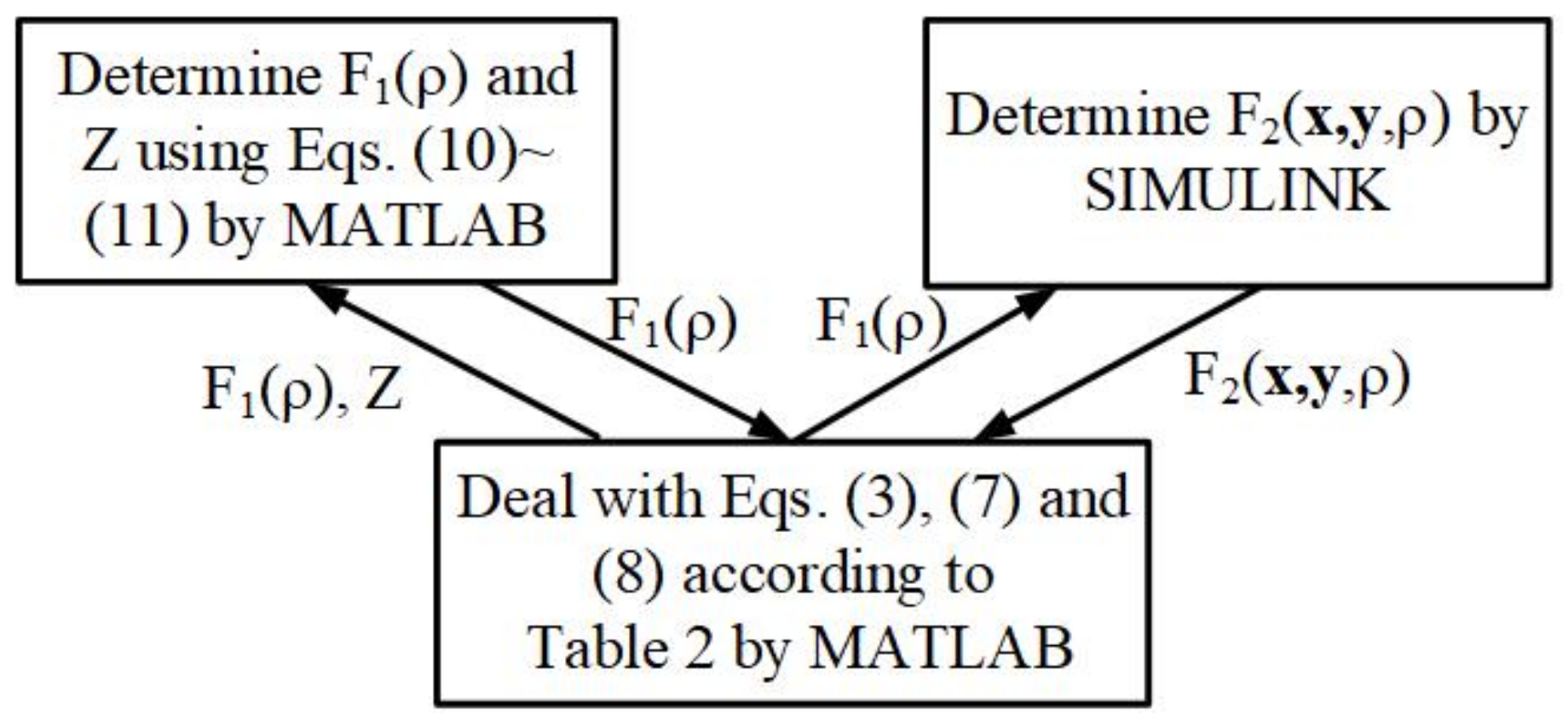
- Particle swarm optimization (PSO) is employed to minimize the shed loads and maximize the frequency nadir without estimating power deficiency. This can be achieved by a co-simulation between a MATLAB code and Simulink time-domain simulation. Because the number of unknown variables is limited, the number of population size in PSO can be set at a small value to alleviate computational burden.
- (b)
- Only the status of breakers at the generators and the net power load, excluding renewable power generation, are utilized to identify the forced outage without the use of an extra detection or classification algorithm to reduce computation time. The aforementioned information is generally available in a dispatch center; matching data in a look-up table is faster than running complex detection or classification algorithms.
- (c)
- Parallel computation and initialization are implemented in the MATLAB/Simulink to reduce the computational burden. Specifically, the result of a normal base case scenario serves as an initial condition for the corresponding contingency cases to greatly reduce the time-domain simulation. Moreover, all contingencies and all particle studies in PSO are mutually independent; thus, they can be studied in parallel using multi-core in a CPU of a personal computer.
2. Description and Formulation of Problem
2.1. Difference between Event-Based and Response-Driven UFLS Schemes
- An event-based UFLS scheme has a single stage in which loads are shed immediately after a pre-specified outage occurs while a response-driven UFLS scheme comprises multiple stages with various frequency thresholds and time delays.
- An event-based UFLS scheme generally requires a communication system to identify or detect pre-specified events while a response-driven UFLS scheme needs local frequency measurements at load buses.
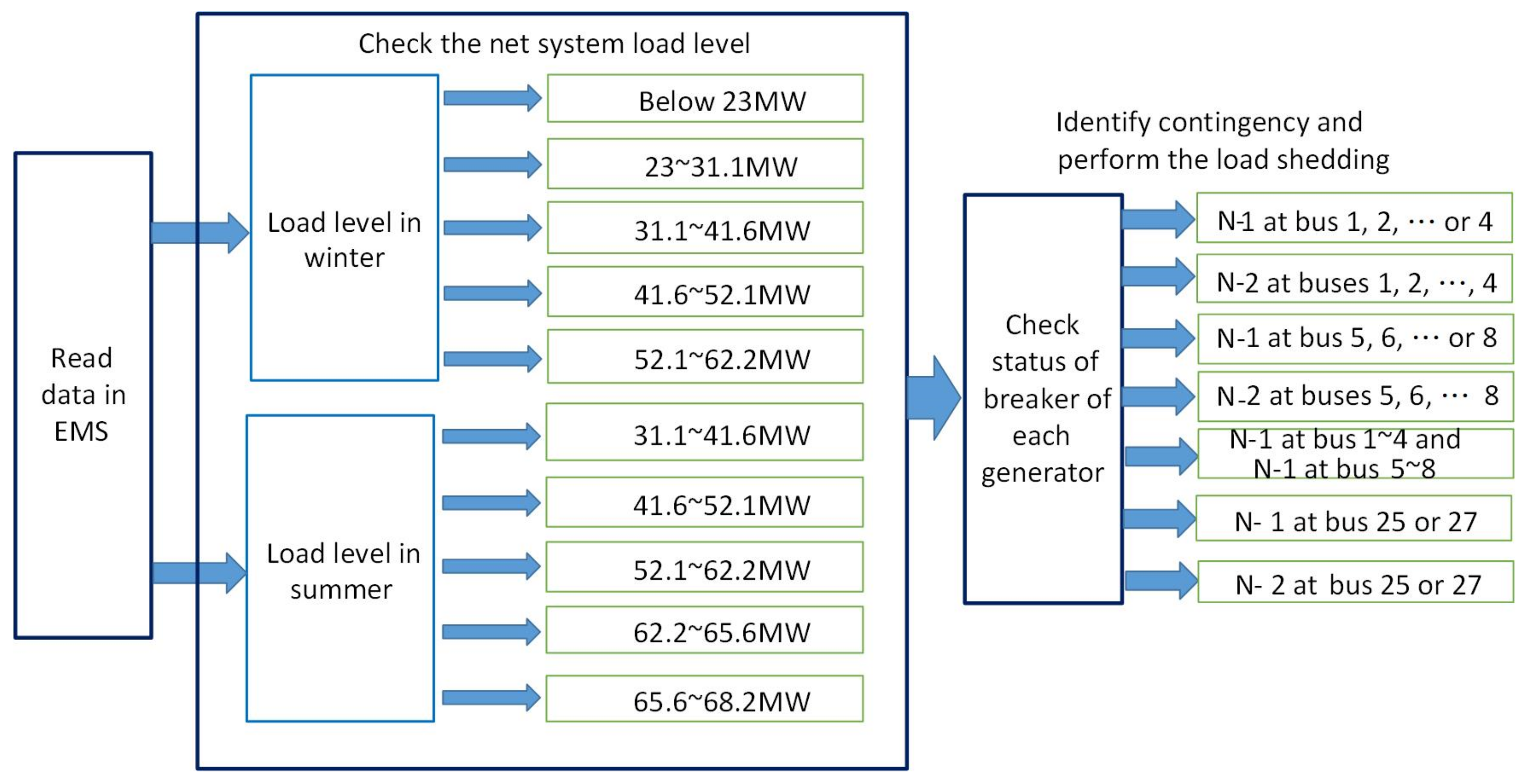
- An event-based UFLS scheme is implemented using a look-up table in an energy management system (EMS) while a response-driven UFLS scheme is realized using local digital relays, such as the 81L relay.
- The common communication system that is needed in the event-based UFLS scheme is ready in utilities; thus, no additional work is required. However, the latency that arises from the communication system must be reduced as much as possible. The triggering time for load shedding is typically 0.2–0.3 s, which includes local fault detection in protection relays and switch devices, and the communication latency from the control center to the breakers [23]. Thus, additional detection or classification algorithm must be avoided.
- Once a response-driven UFLS scheme is implemented, a latent cascading unanticipated outage at a renewable generation resource is most likely to happen. For example, the under-frequency protection of a Vestas V80 wind-turbine generator is set to 58.5 Hz. Before the breakers are open in the first stage (say 57.4 Hz) to shed loads, the wind-turbine generator will automatically trip, causing a more severe frequency nadir. The event-based UFLS scheme can avoid such an unanticipated wind-turbine outage.
- The frequency threshold in the first stage of a response-driven UFLS scheme relies on the power quality requirement in the power system. However, an event-based UFLS scheme activates pre-determined shed loads independently of frequency threshold. Restated, the moment of load shedding in an event-based UFLS scheme is earlier than that in the response-driven one. Accordingly, the frequency nadir that is obtained by an event-based UFLS scheme generally exceeds that by a response-driven UFLS scheme.
- The peak-load scenario is generally considered in developing a response-driven UFLS scheme; the load and power generation pattern in other scenarios are assumed proportional to those in the peak-load scenario to avoid many studies on multiple scenarios. Thus, only the peak-load scenario is studied in the response-driven UFLS scheme. However, this assumption may not hold in a power system with a high penetration of photovoltaic power and wind power because the power generation from renewables is extremely uncertain. To deal with this situation, multi-scenario considering stochastic (probabilistic) models shall be explored to develop the response-driven UFLS scheme.
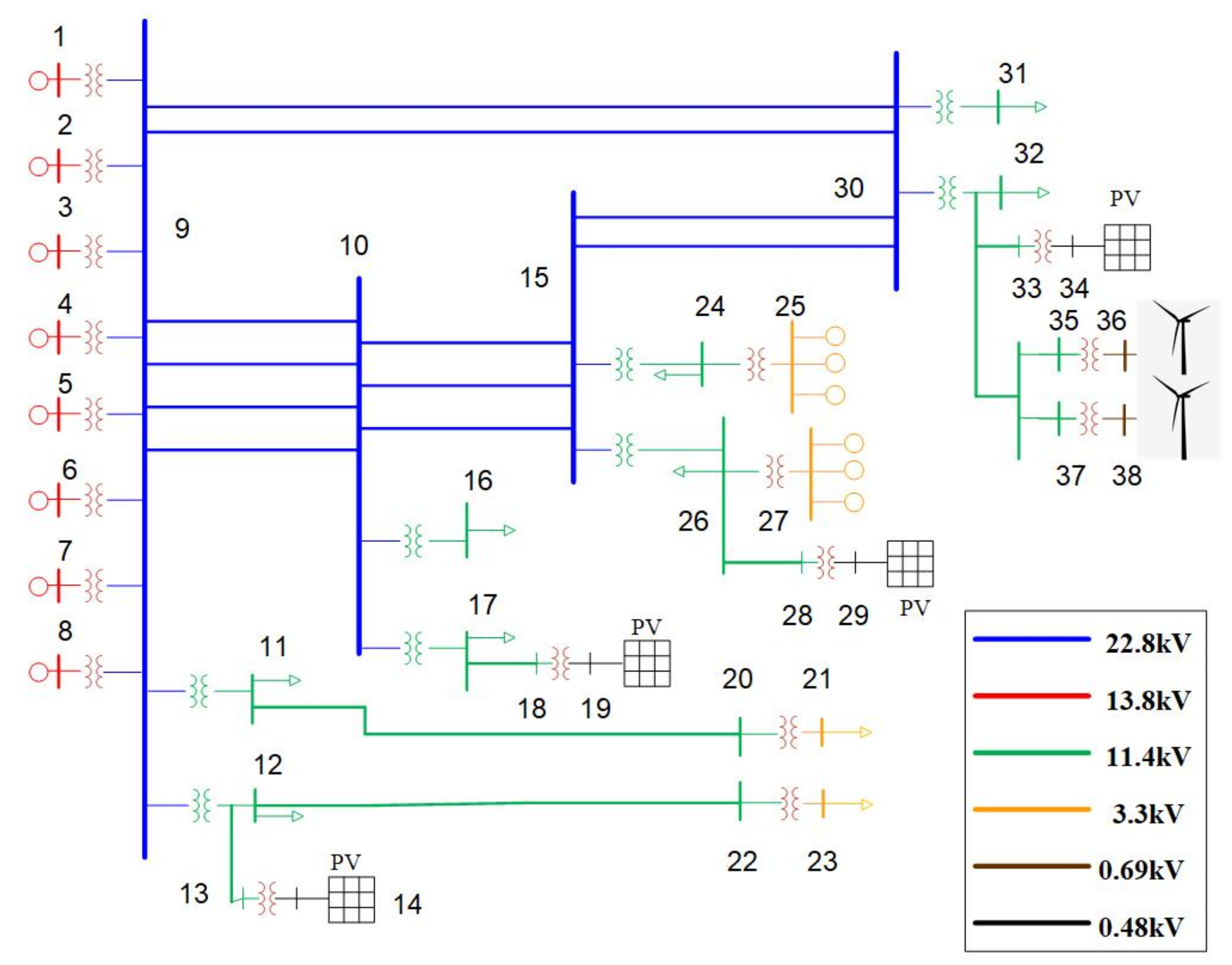
2.2. Studied Standalone Power System
2.3. Problem Formulation of a Single Event
3. Proposed Method
3.1. Pareto Optimum
3.2. Particle Swarm Optimization
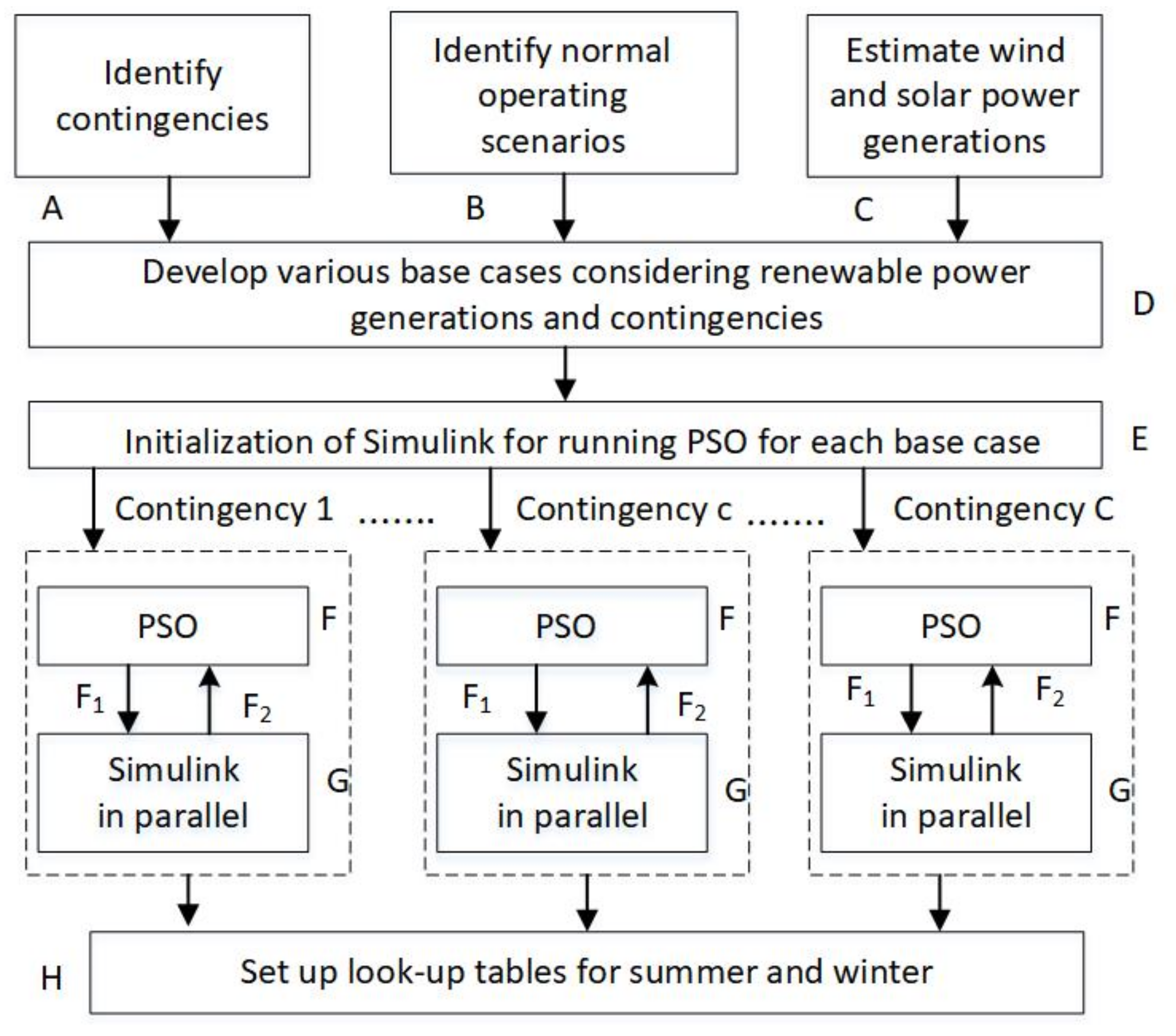
3.3. Initialization and Parallel Computing
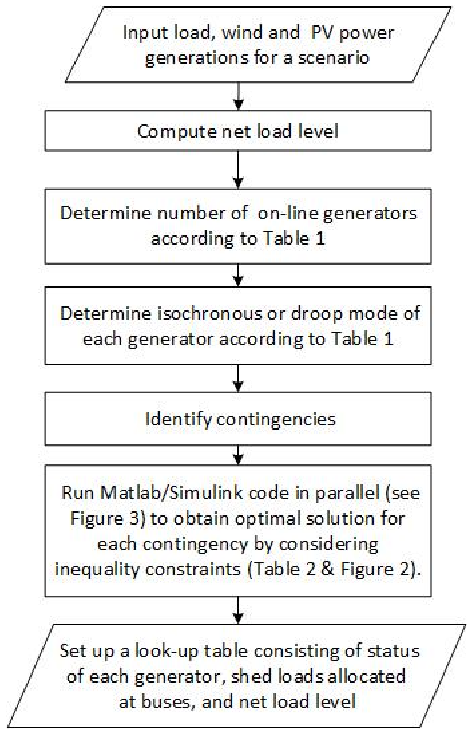
3.3.1. Initialization
3.3.2. Parallel Computing
3.4. Block Diagram of Proposed Method
4. Simulation Results
4.1. Base-Case Scenarios and Contingencies
4.2. Optimization of UFLS
4.3. Comparison of Results Obtained Using Electric Utility Method, Singh’s Method and Proposed Method
4.4. Discussions
- (1)
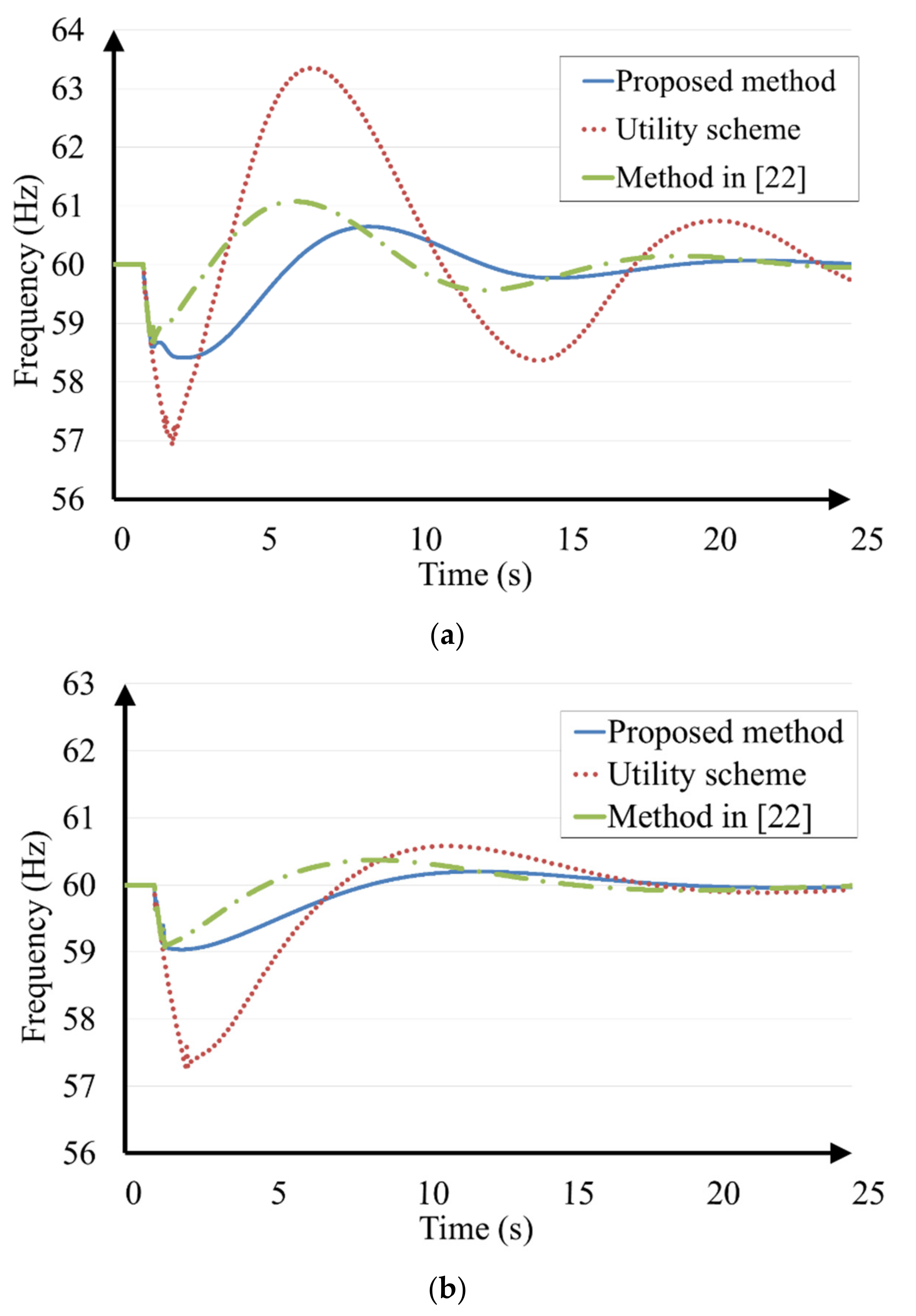
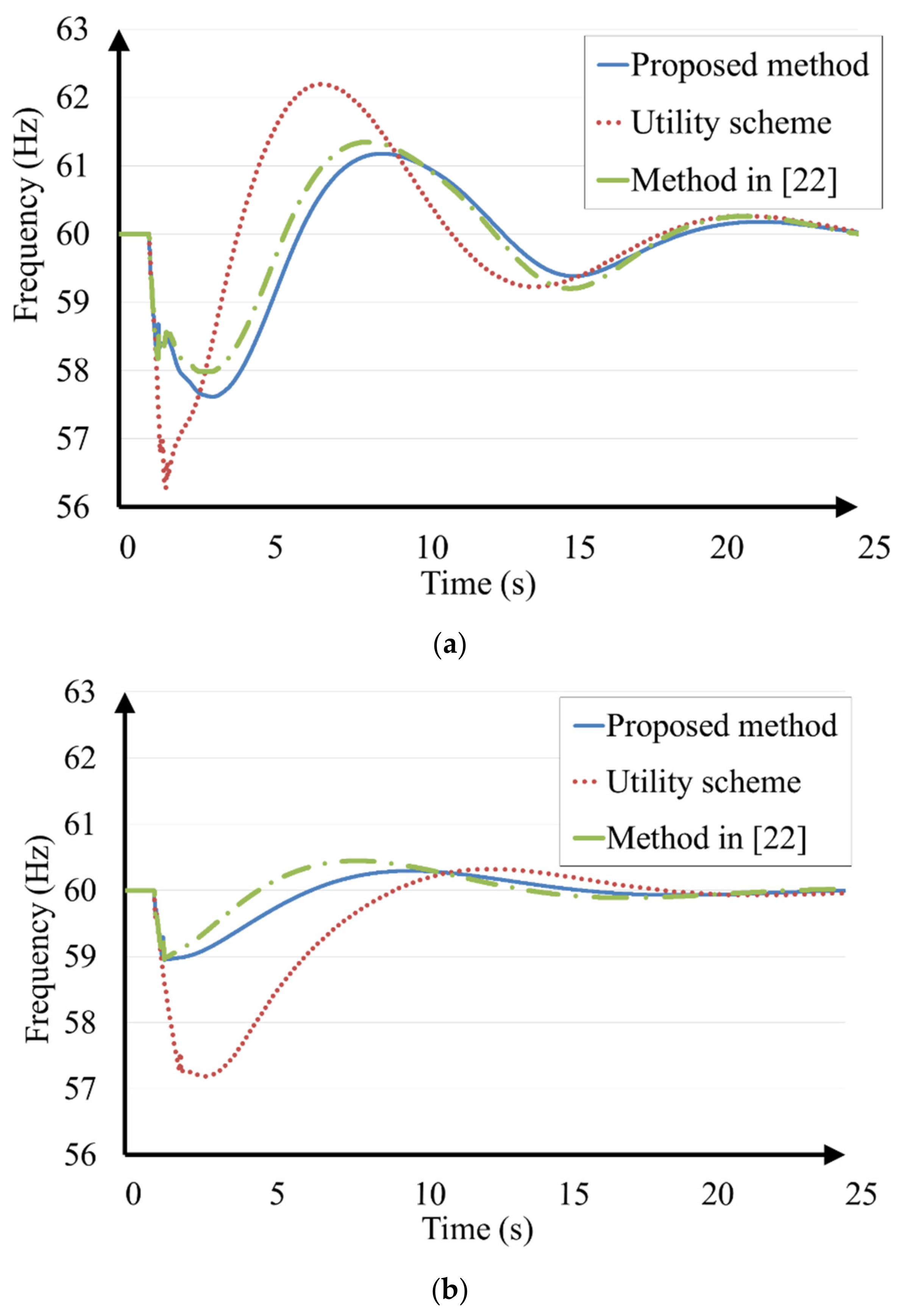
- PSO is able to obtain smaller shed loads than those obtained by the method in [22]. PSO is also attains a smaller shed load in scenarios s1, s5, and w1 associating with the most severe N-2 contingency at buses 5 and 6 than the utility method. It can be found that the frequency nadirs obtained by the proposed method are higher than those by the utility method; the frequency nadirs obtained by the proposed method are very close to those by the method in [22]. All these evidences imply that PSO implemented in the proposed method is crucial.
- (2)
- According to Table 5 and Table 6, in additional to the net load levels in summer or winter, the number of status of breakers at generators, which are required in the look-up table, are few: (i) 8 at buses 1–8 and 3 at buses 25 and 27 in summer, (ii) 7 at buses 1~8 and 2 at buses 25 and 27. Accordingly, it is easy to implement the event-based UFLS scheme in a standalone power system without the use of a complex detection or classification algorithm.
- (3)
- When a MATLAB/Simulink time-domain simulation is carried out, it generally needs simulation time of 60 s to approach to a steady state due to a default initial condition. Thus, any occurrence of a forced outage may be set at 60 s and it takes more time, say 25 s (see Figure 6 and Figure 7), to approach to a new steady state. Thus, the optimal result of a normal condition obtained by PSO at 60 s may serve as an initial condition for all corresponding forced outages with the same net load level. A PSO considering 10 particles generally needs 20 iterations to attain an optimal solution. For the summer season, 15 contingencies require PSO studies (see Table 9). If all initial conditions of scenarios s1~s5 are ready, then total period of time-domain simulation is estimated to be 25 s × 10 × 20 × 15 (75,000 s = 20.83 h). If a 4-core CPU in a computer is used for parallel computing, then the period can be reduced to 18,750 s. However, if initial conditions and parallel computing are not implemented, then total period of the time-domain simulation is about 85 s × 10 × 20 × 15 (255,000 s = 70.83 h).
- (4)
- The proposed method can be applied to large-scale power systems with high penetration of renewable energies. Rather than diesel generators with isochronous control modes in a standalone power grid, combined cycle generators are used in a large power system to compensate the power deficit quickly. The average mode-based time-domain simulation tool (such as PSS/E) can be used to calculate the effective values of all state variables to save computational time. This time-domain simulation tool can be integrated with a Python-based PSO. Moreover, the net load levels, the number of status of breakers at generators and shed loads allocated at buses are required to build up a look-up table.
5. Conclusions
Author Contributions
Funding
Institutional Review Board Statement
Informed Consent Statement
Data Availability Statement
Conflicts of Interest
Nomenclature
| Abbreviations: | |
| CPU | central processing unit |
| EMS | energy management system |
| ICON | isochronous control |
| MBASE | MW base |
| PELEC | electric real power |
| PMECH | mechanical power |
| PMU | phase measurement unit |
| PSO | particle swarm optimization |
| PV | photovoltaic |
| RoCoF | rate of change of frequency (Hz/s) |
| SBASE | apparent power base |
| UFLS | under-frequency load shedding |
| WAMS | wide-area measurement system |
| Indices: | |
| p | index for a particle, p = 1, 2, …, P (P = 10) |
| s1~s5 | scenario indices for summer |
| t | iteration index in PSO |
| w1~w5 | scenario indices for winter |
| Parameters: | |
| and | positive learning factors between 0 and 2 |
| the expected value for , = 1, 2 | |
| , | the maximum and minimum values of |
| , | random numbers within [0, 1] in PSO |
| the weighting factor for , = 1, 2 | |
| ρ | total shed load, the same as |
| the inertia weight in the t-th iteration for PSO | |
| Variables: | |
| the best position of a particle’s neighbors so far in the t-th iteration for PSO | |
| the best position of a particle in the t-th iteration for PSO | |
| -dimensional velocity vector of particle p | |
| x | the vector of the dynamic state variables, such as the angles and velocities of synchronous machines |
| -dimensional position vector of particle p | |
| y | the vector of algebraic state variables, such as bus voltages |
| Z | the least upper bound of the multiple objective values |
| Functions: | |
| a scale function for the total shed load | |
| the frequency nadir | |
Appendix A


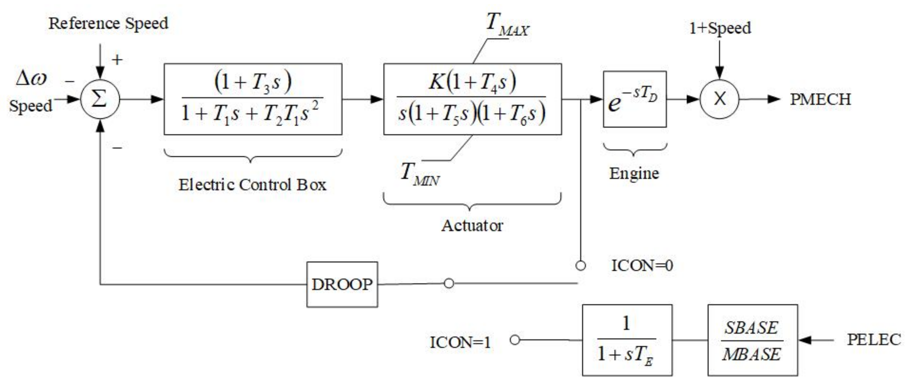
| Parameters | Buses 1–4 | Buses 5–8 | Buses 25, 27 |
|---|---|---|---|
| T1 | 0 | 0 | 0 |
| T2 | 0 | 0 | 0 |
| T3 | 0 | 0 | 0 |
| K | 1.2 | 1.5 | 0.1 |
| T4 | 0.2 | 0.8 | 0 |
| T5 | 0.17 | 0.17 | 1 |
| T6 | 0 | 0 | 0 |
| TD | 0.055 | 0.045 | 0.055 |
| TMAX | 1 | 1 | 1 |
| TMIN | 0.06 | 0 | 0.06 |
| Droop | 0.05 | N/A | 0.05 |
| TE | 0.15 | N/A | 0.15 |
References
- Saparia, N.M.; Mokhlis, H.; Laghari, J.A.; Bakar, A.H.A.; Dahalan, M.R.M. Application of load shedding schemes for distribution network connected with distributed generation: A review. Renew. Sustain. Energy Rev. 2018, 82, 858–867. [Google Scholar] [CrossRef]
- Lai, C.Y.; Liu, C.W. A Scheme to mitigate generation trip events by ancillary services considering minimal actions of UFLS. IEEE Trans. Power Syst. 2020, 35, 4815—4823. [Google Scholar] [CrossRef]
- Rudez, U.; Mihalic, R. WAMS-based underfrequency load shedding with short-term frequency prediction. IEEE Trans. Power Deliv. 2016, 31, 1912–1920. [Google Scholar] [CrossRef]
- Chandra, A.; Pradhan, A.K. An adaptive underfrequency load shedding scheme in the presence of solar photovoltaic plants. IEEE Syst. J. 2021, 15, 1235–1244. [Google Scholar] [CrossRef]
- Karimi, M.; Wall, P.; Mokhlis, H.; Terzija, V. A new centralized adaptive underfrequency load shedding controller for microgrids based on a distribution state estimator. IEEE Trans. Power Deliv. 2017, 32, 370–380. [Google Scholar] [CrossRef]
- Xu, Q.; Yang, B.; Chen, C.; Lin, F.; Guan, X. Distributed load shedding for microgrid with compensation support via wireless network. IET Gener. Transm. Distrib. 2018, 12, 2006–2018. [Google Scholar] [CrossRef] [Green Version]
- Talaat, M.; Hatata, A.Y.; Alsayyari, A.S.; Alblawi, A. A smart load management system based on the grasshopper optimization algorithm using the under-frequency load shedding approach. Energy 2020, 190, 116423. [Google Scholar] [CrossRef]
- Amraee, T.; Darebaghi, M.G.; Soroudi, A.; Keane, A. Probabilistic under frequency load shedding considering RoCoF relays of distributed generators. IEEE Trans. Power Syst. 2018, 33, 3587–3598. [Google Scholar] [CrossRef] [Green Version]
- Banijamali, S.S.; Amraee, T. Semi-adaptive setting of under frequency load shedding relays considering credible generation outage scenarios. IEEE Trans. Power Deliv. 2019, 34, 1098–1108. [Google Scholar] [CrossRef]
- Laghari, J.A.; Mokhlis, H.; Karimi, M.; Bakar, A.H.A.; Mohamad, H. A new under-frequency load shedding technique based on combination of fixed and random priority of loads for smart grid applications. IEEE Trans. Power Syst. 2015, 30, 2507–2515. [Google Scholar] [CrossRef]
- Das, K.; Nitsas, A.; Altin, M.; Hansen, A.D.; Sørensen, P.E. Improved load-shedding scheme considering distributed generation. IEEE Trans. Power Deliv. 2017, 32, 515–524. [Google Scholar] [CrossRef]
- Li, C.; Wu, Y.; Sun, Y.; Zhang, H.; Liu, Y.; Liu, Y.; Terzija, V. Continuous under-frequency load shedding scheme for power system adaptive frequency control. IEEE Trans. Power Syst. 2020, 35, 950–961. [Google Scholar] [CrossRef]
- Darebaghi, M.G.; Amraee, T. Dynamic multi-stage under frequency load shedding considering uncertainty of generation loss. IET Gener. Transm. Distrib. 2017, 11, 3202–3209. [Google Scholar] [CrossRef]
- Acosta, M.N.; Adiyabazar, C.; Gonzalez-Longatt, F.; Andrade, M.A.; Torres, J.R.; Vazquez, E.; Riquelme Santos, J.M. Optimal under-frequency load shedding setting at Altai-Uliastai regional power system, Mongolia. Energies 2020, 13, 5390. [Google Scholar] [CrossRef]
- Rudez, U.; Mihalic, R. Predictive underfrequency load shedding scheme for islanded power systems with renewable generation. Electr. Power Syst. Res. 2015, 126, 21–28. [Google Scholar] [CrossRef]
- Khezri, R.; Golshannavaz, S.; Vakili, R.; Memar-Esfahani, B. Multi-layer fuzzy-based under-frequency load shedding in back-pressure smart industrial microgrids. Energy 2017, 132, 96–105. [Google Scholar] [CrossRef]
- Zhou, Q.; Li, Z.; Wu, Q.; Shahidehpour, M. Two-stage load shedding for secondary control in hierarchical operation of islanded microgrids. IEEE Trans. Smart Grid 2019, 10, 3103–3111. [Google Scholar] [CrossRef] [Green Version]
- Dehghanpour, E.; Karegar, H.K.; Kheirollahi, R. Under frequency load shedding in inverter based microgrids by using droop characteristic. IEEE Trans. Power Deliv. 2021, 36, 1097–1106. [Google Scholar] [CrossRef]
- Nascimento, B.N.; Souza, A.C.Z.; Costa, J.G.C.; Castilla, M. Load shedding scheme with under-frequency and undervoltage corrective actions to supply high priority loads in islanded microgrids. IET Renew. Power Gener. 2019, 13, 1981–1989. [Google Scholar] [CrossRef] [Green Version]
- Shi, F.; Zhang, H.; Cao, Y.; Sun, H.; Chai, Y. Enhancing event-driven load shedding by corrective switching with transient security and overload constraints. IEEE Access 2019, 7, 101355–101365. [Google Scholar] [CrossRef]
- Shekari, T.; Gholami, A.; Aminifar, F.; Sanaye-Pasand, M. An adaptive wide-area load shedding scheme incorporating power system real-time limitations. IEEE Syst. J. 2018, 12, 759–767. [Google Scholar] [CrossRef]
- Singh, A.K.; Fozdar, M. Event-driven frequency and voltage stability predictive assessment and unified load shedding. IET Gener. Transm. Distrib. 2019, 13, 4410–4420. [Google Scholar] [CrossRef]
- Xu, X.; Zhang, H.; Li, C.; Liu, Y.; Li, W.; Terzija, V. Optimization of the event-driven emergency load-shedding considering transient security and stability constraints. IEEE Trans. Power Syst. 2017, 32, 2581–2592. [Google Scholar] [CrossRef]
- Yeh, C.C.; Chen, C.S.; Ku, T.T.; Lin, C.H.; Hsu, C.T.; Chang, Y.R.; Lee, Y.D. Design of special protection system for an offshore island with high-PV penetration. IEEE Trans. Ind. Appl. 2017, 53, 947–953. [Google Scholar] [CrossRef]
- Padrón, S.; Hernández, M.; Falcón, A. Reducing under-frequency load shedding in isolated power systems using neural networks. Gran Canaria: A case study. IEEE Trans. Power Syst. 2016, 31, 63–71. [Google Scholar] [CrossRef]
- Laghari, A.; Mokhlis, H.; Halim Abu Bakar, A.B.; Karimi, M.; Shahriari, A. An intelligent under frequency load shedding scheme for an islanded distribution network. In Proceedings of the 2012 IEEE International Power Engineering and Optimization Conference, Melaka, Malaysia, 6–7 June 2012; pp. 40–45. [Google Scholar] [CrossRef]
- Mokhlis, H.; Laghari, J.A.; Bakar, A.H.A.; Karimi, M. A fuzzy based under-frequency load shedding scheme for islanded distribution network connected with DG. Int. Rev. Electr. Eng. 2012, 7, 4992–5000. [Google Scholar]
- Mahat, P.; Chen, Z.; Bak-Jensen, B. Underfrequency load shedding for an islanded distribution system with distributed generators. IEEE Trans. Power Deliv. 2010, 25, 911–918. [Google Scholar] [CrossRef]
- Worku, M.Y.; Hassan, M.A.; Abido, M.A. Real time energy management and control of renewable energy based microgrid in grid connected and island modes. Energies 2019, 12, 276. [Google Scholar] [CrossRef] [Green Version]
- Bakar, N.N.A.; Hassan, M.Y.; Sulaima, M.F.; Nasir, M.N.M.; Khamis, A. Microgrid and load shedding scheme during islanded mode: A review. Int. J. Renew. Sustain. Energy Rev. 2017, 71, 161–169. [Google Scholar] [CrossRef]
- Ammar, E.I. Interactive stability of multi-objective NLP problems with fuzzy parameters in the objective functions and constraints. Fuzzy Sets Syst. 2000, 109, 83–90. [Google Scholar] [CrossRef]
- Chankong, V.; Haimes, Y. Multiobjective Decision Making: Theory and Methodology; North-Holland: New York, NY, USA, 1983. [Google Scholar]
- Kalinović, S.M.; Tanikić, D.I.; Djoković, J.M.; Nikolić, R.R.; Hadzima, B.; Ulewicz, R. Optimal solution for an energy efficient construction of a ventilated façade obtained by a genetic algorithm. Energies 2021, 14, 3293. [Google Scholar] [CrossRef]
- Kennedy, J.; Eberhart, R. Particle swarm optimization. In Proceedings of the IEEE Int. Conf. on Neural Networks, Perth, WA, Australia, 27 November–1 December 1995; Volume 4, pp. 1942–1948. [Google Scholar]
- Deng, C.; Zhang, X.; Huang, Y.; Bao, Y. Equipping seasonal exponential smoothing models with particle swarm optimization algorithm for electricity consumption forecasting. Energies 2021, 14, 4036. [Google Scholar] [CrossRef]
- PSS/E 34 Users Manual; Siemens Industry Inc.: Erlangen, Germany, 2020.


| Net Load Level | Buses 25 and 27 | Buses 1~4 | Buses 5~8 |
|---|---|---|---|
| droop mode | droop mode | isochronous mode | |
| scheduled power × quantity | scheduled power × quantity | ||
| –20.4 MW | 0 | 5.1 MW × 4 | |
| 20.401–23.0 MW | 2.6 MW × 1 | 5.1 MW × 4 | |
| 23.001–31.1 MW | 2.6 MW × 1 | 5.7 MW × 5 | |
| 31.101–41.6 MW | 2.6 MW × 1 | 6.5 MW × 6 | |
| 41.601–52.1 MW | 2.6 MW × 2 | 6.7 MW × 7 | |
| 52.101–62.2 MW | 2.6 MW × 3 | 6.8 MW × 8 | |
| 62.201–65.6 MW | 2.6 MW × 4 | 6.9 MW × 8 | |
| 65.601–68.2 MW | 2.6 MW × 5 | 6.9 MW × 8 | |
| Condition | Treatment |
|---|---|
| Violation of Equation (7) or (8) | Z = maximum of and |
| Scenario | Total Power of Diesel Generators | Load Level | Wind Power | PV Power | Net Load Level |
|---|---|---|---|---|---|
| s1 | 31.101–41.60 | 33.36 | 4.0 | 0.0 | 29.36 |
| s2 | 41.601–52.10 | 46.85 | 3.0 | 1.9 | 41.95 |
| s3 | 41.601–52.10 | 57.15 | 2.0 | 3.8 | 51.35 |
| s4 | 52.101–62.20 | 63.90 | 1.0 | 5.7 | 57.20 |
| s5 | 52.101–62.20 | 66.62 | 0.0 | 7.6 | 59.02 |
| Scenario | Total Power of Diesel Generators | Load Level | Wind Power | PV Power | Net Load Level |
|---|---|---|---|---|---|
| w1 | –20.04 | 22.80 | 4.0 | 0.0 | 18.80 |
| w2 | 20.401–23.00 | 27.05 | 3.0 | 1.9 | 22.15 |
| w3 | 23.001–31.10 | 36.35 | 2.0 | 3.8 | 30.55 |
| w4 | 31.101–41.60 | 46.85 | 1.0 | 5.7 | 40.15 |
| w5 | 41.601–52.10 | 55.53 | 0.0 | 7.6 | 47.93 |
| Scenario | Buses 1–4 with Droop Mode | Buses 5–8 with Isochronous Mode | Buses 25 and 27 with Droop Mode |
|---|---|---|---|
| s1 | 5.7 × 1 (MW) | 5.7 × 4 (MW) | 2.6 × 1 (MW) |
| s2 | 6.7 × 3 (MW) | 6.7 × 4 (MW) | 2.6 × 2 (MW) |
| s3 | 6.7 × 3 (MW) | 6.7 × 4 (MW) | 2.6 × 2 (MW) |
| s4 | 6.8 × 4 (MW) | 6.8 × 4 (MW) | 2.6 × 3 (MW) |
| s5 | 6.8 × 4 (MW) | 6.8 × 4 (MW) | 2.6 × 3 (MW) |
| Scenario | Buses 1–4 with Droop Mode | Buses 5–8 with Isochronous Mode | Buses 25 and 27 with Droop Mode |
|---|---|---|---|
| w1 | 5.1 × 1 (MW) | 5.1 × 3 (MW) | 0 (MW) |
| w2 | 5.1 × 1 (MW) | 5.1 × 3 (MW) | 2.6 × 1 (MW) |
| w3 | 5.7 × 1 (MW) | 5.7 × 4 (MW) | 2.6 × 1 (MW) |
| w4 | 6.5 × 2 (MW) | 6.5 × 4 (MW) | 2.6 × 1 (MW) |
| w5 | 6.7 × 3 (MW) | 6.7 × 4 (MW) | 2.6 × 2 (MW) |
| Scenario | N-1 at Bus 1 | N-1 at Bus 5 | N-2 at Buses 1 and 2 | N-2 at Buses 5 and 6 | N-1 at Bus 25 | N-2 at Bus 25 | N-1 at Bus 1; N-1 at Bus 5 |
|---|---|---|---|---|---|---|---|
| s1 | 57.29 | 56.98 | - | 44.99 | 58.88 | - | 51.41 |
| s2 | 57.50 | 58.15 | 55.28 | 55.92 | 59.05 | 58.17 | 55.64 |
| s3 | 57.63 | 57.41 | 55.36 | 51.06 | 59.10 | 58.34 | 53.03 |
| s4 | 57.66 | 57.92 | 55.72 | 55.76 | 59.16 | 58.32 | 55.70 |
| s5 | 57.82 | 57.78 | 53.89 | 50.85 | 59.17 | 58.33 | 52.39 |
| Scenario | N-1 at Bus 1 | N-1 at Bus 5 | N-2 at Buses 1 and 2 | N-2 at Buses 5 and 6 | N-1 at Bus 25 | N-2 at Bus 25 | N-1 at Bus 1; N-1 at Bus 5 |
|---|---|---|---|---|---|---|---|
| w1 | 56.58 | 55.94 | - | 44.99 | - | - | 45.15 |
| w2 | 56.91 | 56.56 | - | 44.99 | 58.54 | - | 54.82 |
| w3 | 57.39 | 56.98 | - | 44.99 | 58.92 | - | 58.92 |
| w4 | 57.38 | 57.12 | 55.90 | 54.68 | 59.09 | - | 55.68 |
| w5 | 57.57 | 57.62 | 54.46 | 50.40 | 59.08 | 58.27 | 52.46 |
| Scenarios | Contingencies | Frequency Nadir (Hz) | Shed Load (MW) |
|---|---|---|---|
| s1 | N-1 outage at bus 1 | 59.52 | 5.08 |
| N-1 outage at bus 5 | 59.41 | 6.62 | |
| N-2 outage at buses 5 and 6 | 58.41 | 9.45 | |
| N-1 at bus 1; N-1 at bus 5 | 58.48 | 9.19 | |
| s2 | N-2 outage at buses 1 and 2 | 58.89 | 10.83 |
| N-2 outage at buses 5 and 6 | 59.21 | 8.38 | |
| N-1 at bus 1; N-1 at bus 5 | 59.13 | 9.40 | |
| s3 | N-2 outage at buses 1 and 2 | 59.18 | 11.46 |
| N-2 outage at buses 5 and 6 | 58.88 | 12.80 | |
| N-1 at bus 1; N-1 at bus 5 | 59.05 | 11.84 | |
| s4 | N-2 outage at buses 1 and 2 | 59.22 | 11.82 |
| N-2 outage at buses 5 and 6 | 59.17 | 12.10 | |
| N-1 at bus 1; N-1 at bus 5 | 59.41 | 10.86 | |
| s5 | N-2 outage at buses 1 and 2 | 59.41 | 11.32 |
| N-2 outage at buses 5 and 6 | 59.04 | 10.33 | |
| N-1 at bus 1; N-1 at bus 5 | 59.26 | 12.06 |
| Scenarios | Contingencies | Frequency Nadir (Hz) | Shed Load (MW) |
|---|---|---|---|
| w1 | N-1 outage at bus 1 | 59.30 | 4.22 |
| N-1 outage at bus 5 | 59.24 | 4.61 | |
| N-2 outage at buses 5 and 6 | 57.61 | 8.54 | |
| N-1 at bus 1; N-1 at bus 5 | 57.77 | 8.10 | |
| w2 | N-1 outage at bus 1 | 59.34 | 4.61 |
| N-1 outage at bus 5 | 59.28 | 4.67 | |
| N-2 outage at buses 5 and 6 | 58.01 | 8.85 | |
| N-1 at bus 1; N-1 at bus 5 | 58.16 | 8.38 | |
| w3 | N-1 outage at bus 1 | 59.06 | 10.18 |
| N-1 outage at bus 5 | 58.98 | 9.89 | |
| N-2 outage at buses 5 and 6 | 58.38 | 10.29 | |
| N-1 at bus 1; N-1 at bus 5 | 58.55 | 9.57 | |
| w4 | N-1 outage at bus 1 | 59.58 | 6.18 |
| N-1 outage at bus 5 | 59.43 | 7.16 | |
| N-2 outage at buses 1 and 2 | 58.79 | 11.04 | |
| N-2 outage at buses 5 and 6 | 58.66 | 11.73 | |
| N-1 at bus 1; N-1 at bus 5 | 58.77 | 11.15 | |
| w5 | N-2 outage at buses 1 and 2 | 59.04 | 11.46 |
| N-2 outage at buses 5 and 6 | 58.94 | 10.81 | |
| N-1 at bus 1; N-1 at bus 5 | 59.12 | 11.10 |
| Scenario | Methods | Shed Load (MW) | Frequency Nadir (Hz) | Overshoot Frequency (Hz) | Number of Stages |
|---|---|---|---|---|---|
| s1 | proposed | 9.45 | 58.41 | 60.65 | - |
| utility | 13.31 | 56.92 | 63.35 | 2 | |
| [22] | 11.49 | 58.60 | 61.08 | - | |
| s5 | proposed | 10.33 | 59.04 | 60.20 | - |
| utility | 11.32 | 57.29 | 60.58 | 1 | |
| [22] | 12.12 | 59.08 | 60.37 | - | |
| w1 | proposed | 8.54 | 57.61 | 60.28 | - |
| utility | 13.62 | 56.28 | 62.19 | 3 | |
| [22] | 11.26 | 57.98 | 61.35 | ||
| w5 | proposed | 10.81 | 58.94 | 60.29 | - |
| utility | 9.40 | 57.19 | 60.32 | 1 | |
| [22] | 11.56 | 58.95 | 60.44 | - |
Publisher’s Note: MDPI stays neutral with regard to jurisdictional claims in published maps and institutional affiliations. |
© 2021 by the authors. Licensee MDPI, Basel, Switzerland. This article is an open access article distributed under the terms and conditions of the Creative Commons Attribution (CC BY) license (https://creativecommons.org/licenses/by/4.0/).
Share and Cite
Hong, Y.-Y.; Hsiao, C.-Y. Event-Based Under-Frequency Load Shedding Scheme in a Standalone Power System. Energies 2021, 14, 5659. https://doi.org/10.3390/en14185659
Hong Y-Y, Hsiao C-Y. Event-Based Under-Frequency Load Shedding Scheme in a Standalone Power System. Energies. 2021; 14(18):5659. https://doi.org/10.3390/en14185659
Chicago/Turabian StyleHong, Ying-Yi, and Chih-Yang Hsiao. 2021. "Event-Based Under-Frequency Load Shedding Scheme in a Standalone Power System" Energies 14, no. 18: 5659. https://doi.org/10.3390/en14185659
APA StyleHong, Y.-Y., & Hsiao, C.-Y. (2021). Event-Based Under-Frequency Load Shedding Scheme in a Standalone Power System. Energies, 14(18), 5659. https://doi.org/10.3390/en14185659