
Effect of Individual Volt/var Control Strategies in LINK-Based Smart Grids with a High Photovoltaic Share


Abstract
1. Introduction
2. Materials and Methods
2.1. Methodology
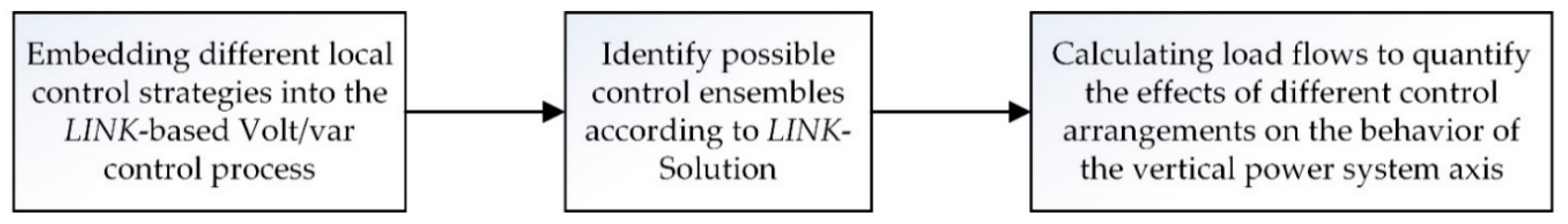
2.1.1. Investigation Methodology
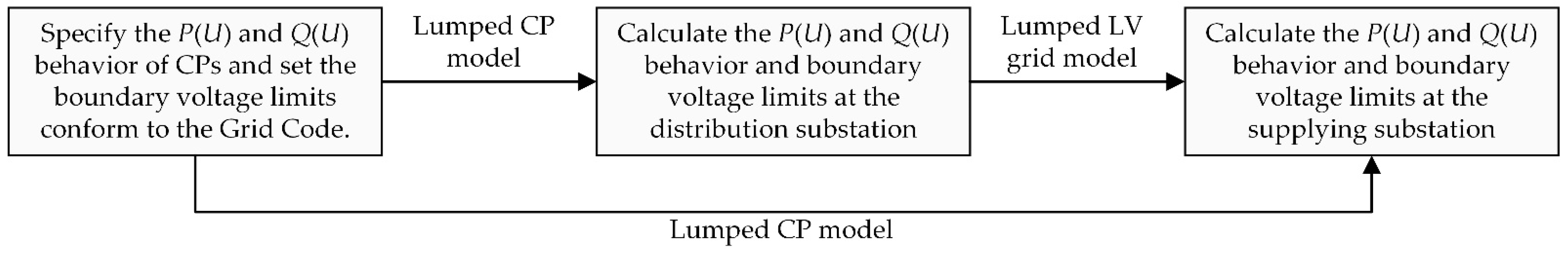
2.1.2. Modeling Procedure
2.2. Generalized Vertical Volt/var Chain Control Scheme
- The voltage set-points for the primary controls of the supplying transformers and other transformers included in the MV_Link-Grid that have OLTC;
- The voltage and reactive power set-points for the primary controls of the producer-links connected to the MV_ Link-Grid;
- The voltage and reactive power set-points for the primary controls of the storage-links connected to the MV_ Link-Grid;
- The voltage, reactive power, and switch position set-points for the primary and direct controls of the RPDs included in the MV_ Link-Grid;
- The reactive power set-points for the secondary controls of the neighboring CP_Grid-Links; and
- The reactive power set-points for the secondary controls of the neighboring LV_Grid-Links;
- The reactive power constraint at the boundary node to the neighboring HV_ Link-Grid.
- The voltage set-points for the primary control of the distribution transformer included in the LV_Link-Grid (when it possesses an OLTC);
- The voltage and reactive power set-points for the primary controls of the producer-links connected to the LV_Link-Grid;
- The voltage and reactive power set-points for the primary controls of the storage-links connected to the LV_Link-Grid;
- The voltage, reactive power, and switch position set-points for the primary and direct controls of the RPDs included in the LV_Link-Grid; and
- The reactive power set-points for the secondary controls of the neighboring CP_Grid-Links;
- The reactive power constraints at the boundary node to the neighboring MV_Link-Grid.
- The voltage and reactive power set-points for the primary controls of the producer-links connected to the CP_Link-Grid;
- The voltage and reactive power set-points for the primary controls of the storage-links connected to the CP_Link-Grid; and
- The switch position set-points for the primary and direct controls of the RPDs included in the CP_Link-Grid;
- The reactive power constraint at the boundary node to the neighboring LV_Link-Grid.
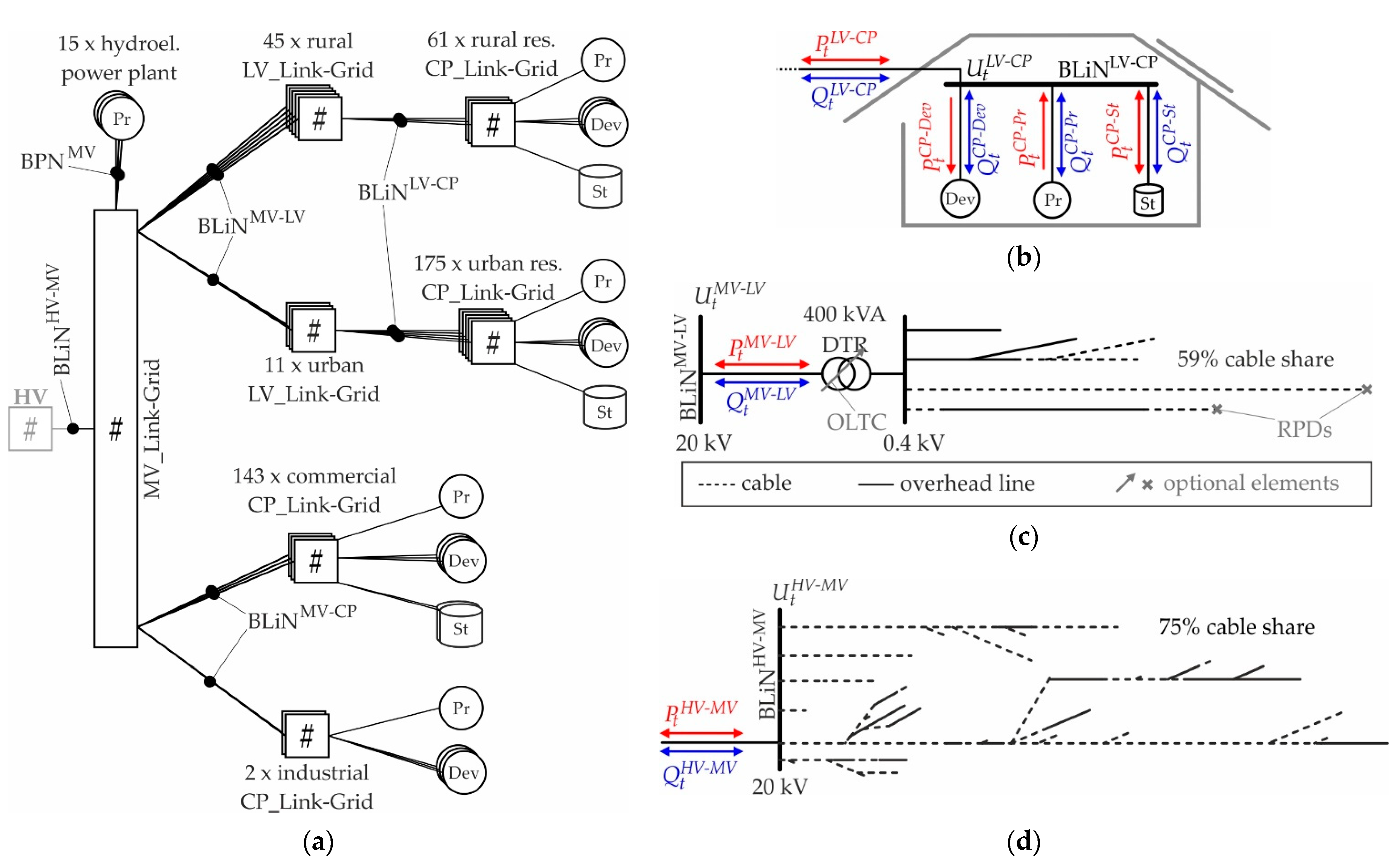
2.3. Description of Test Link-Grids
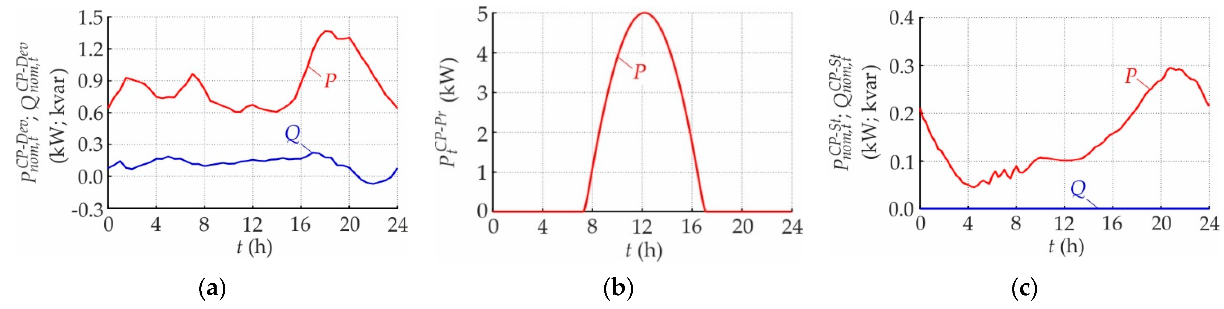
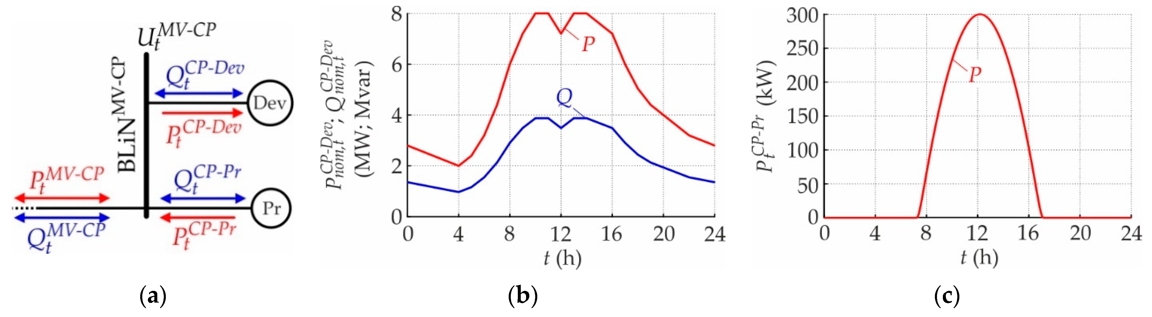
2.3.1. Customer Plant Level
2.3.2. Low Voltage Level
2.3.3. Medium Voltage Level
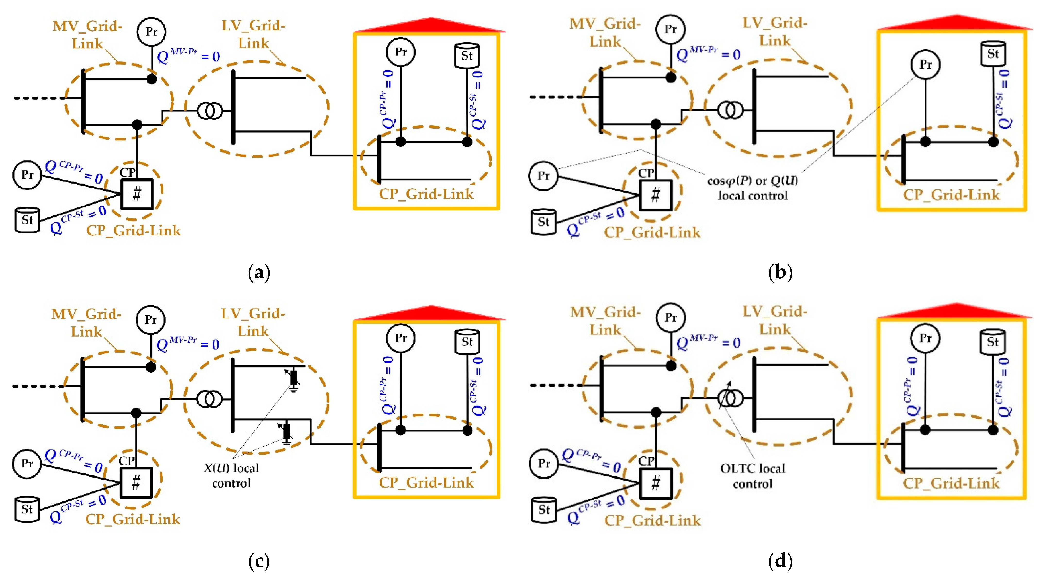
2.4. Description of Volt/var Control Arrangements
2.4.1. No Volt/var Control
2.4.2. Local Controls
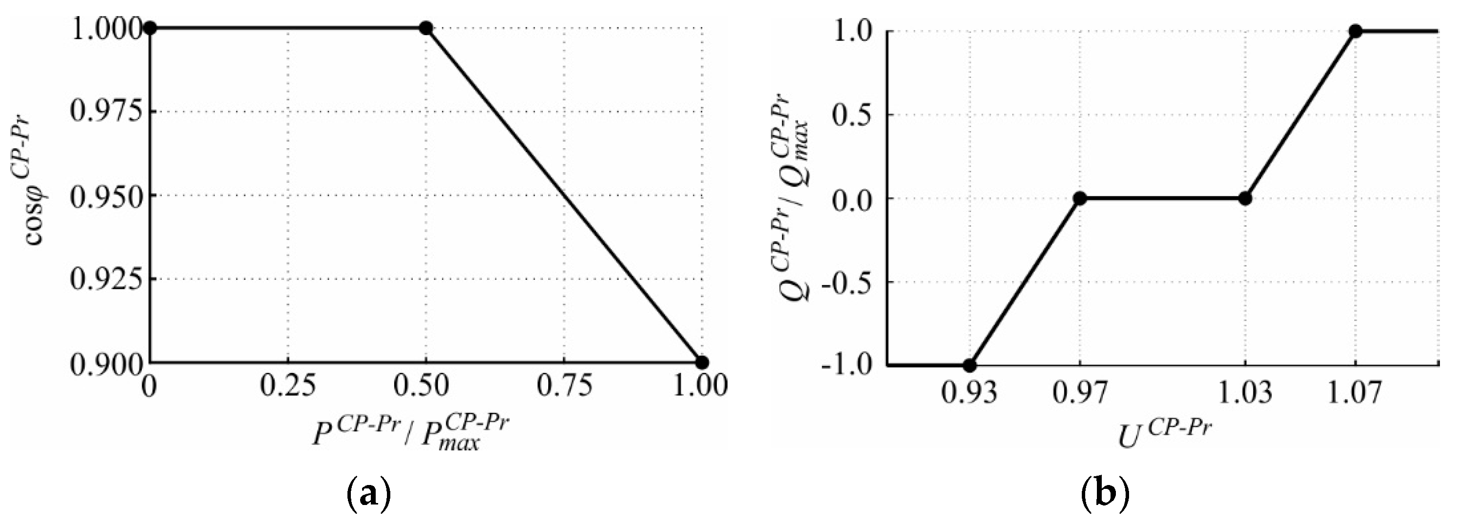
- cosφ(P) control at the CP level
- Q(U) local control at the CP level
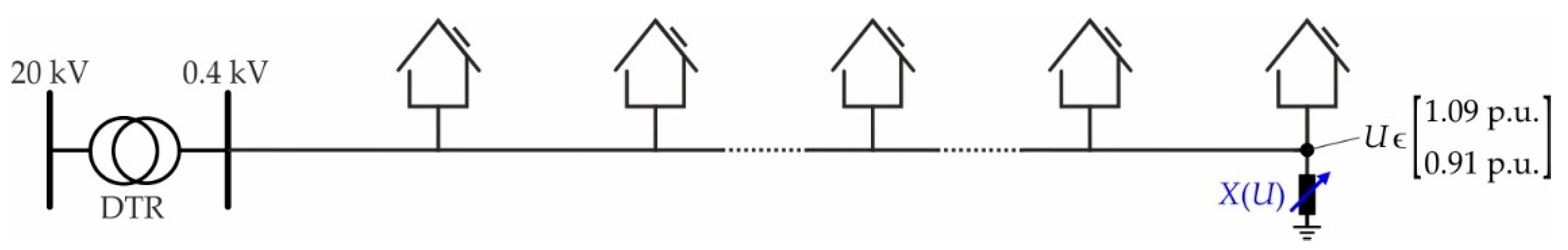
- X(U) local control at the LV level
- OLTC local control at the LV level
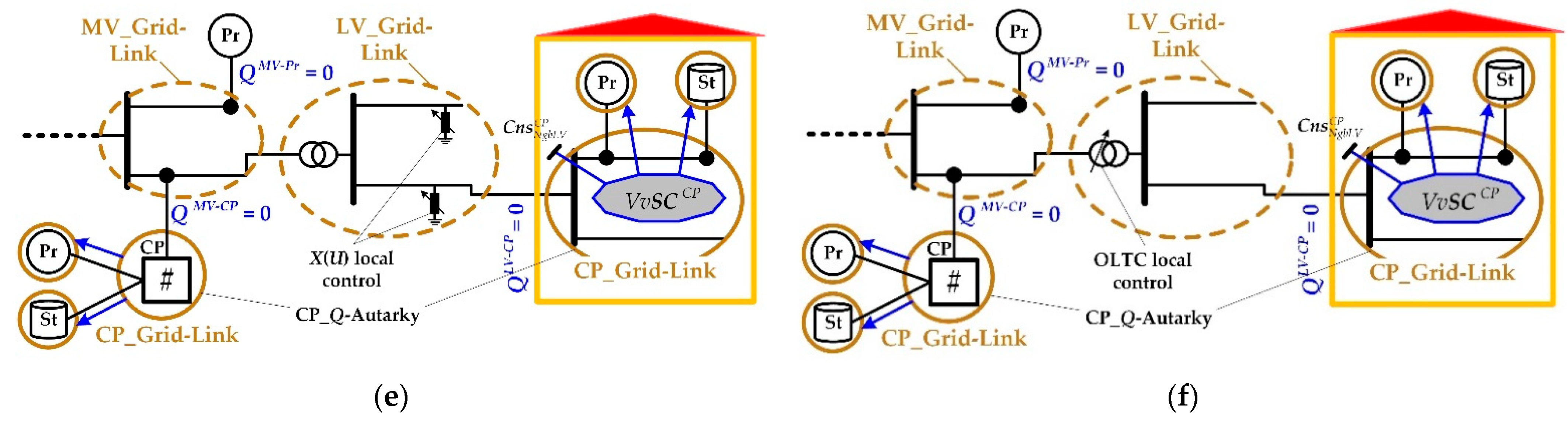
2.4.3. Control Ensembles
- X(U) local control at the LV level and Q-Autarky at the CP level
- OLTC local control at the LV level and Q-Autarky at the CP level
3. Link-Grid Behavior under Different Volt/var Control Arrangements
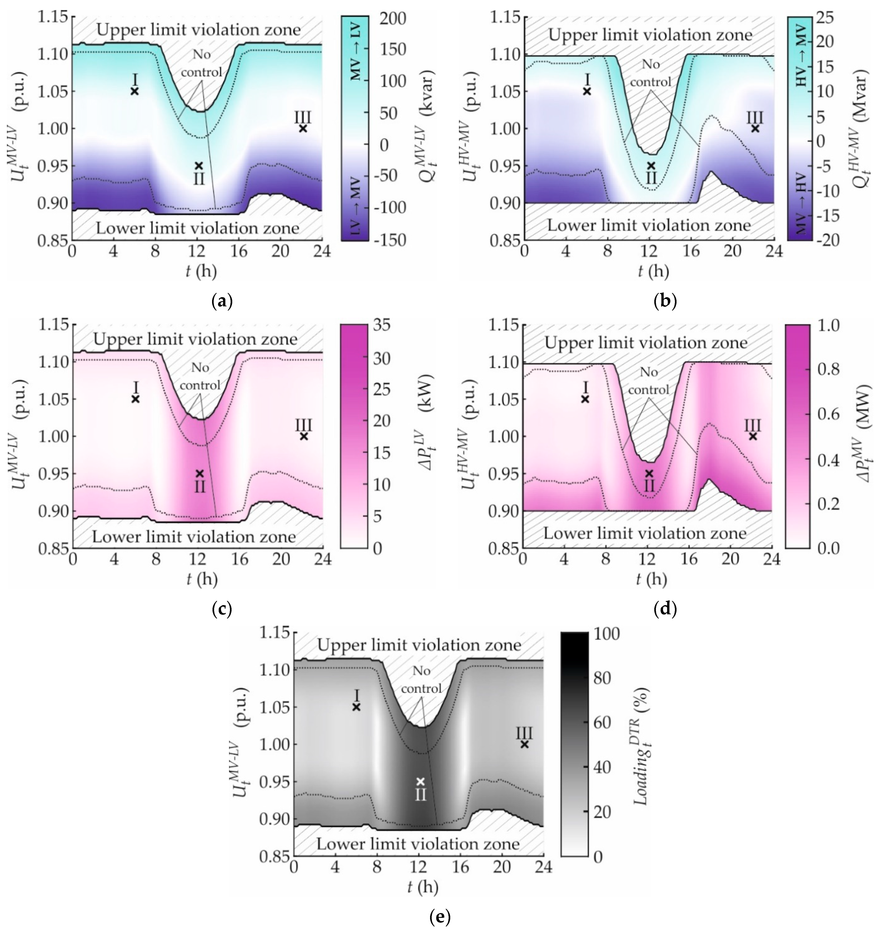
3.1. No Control
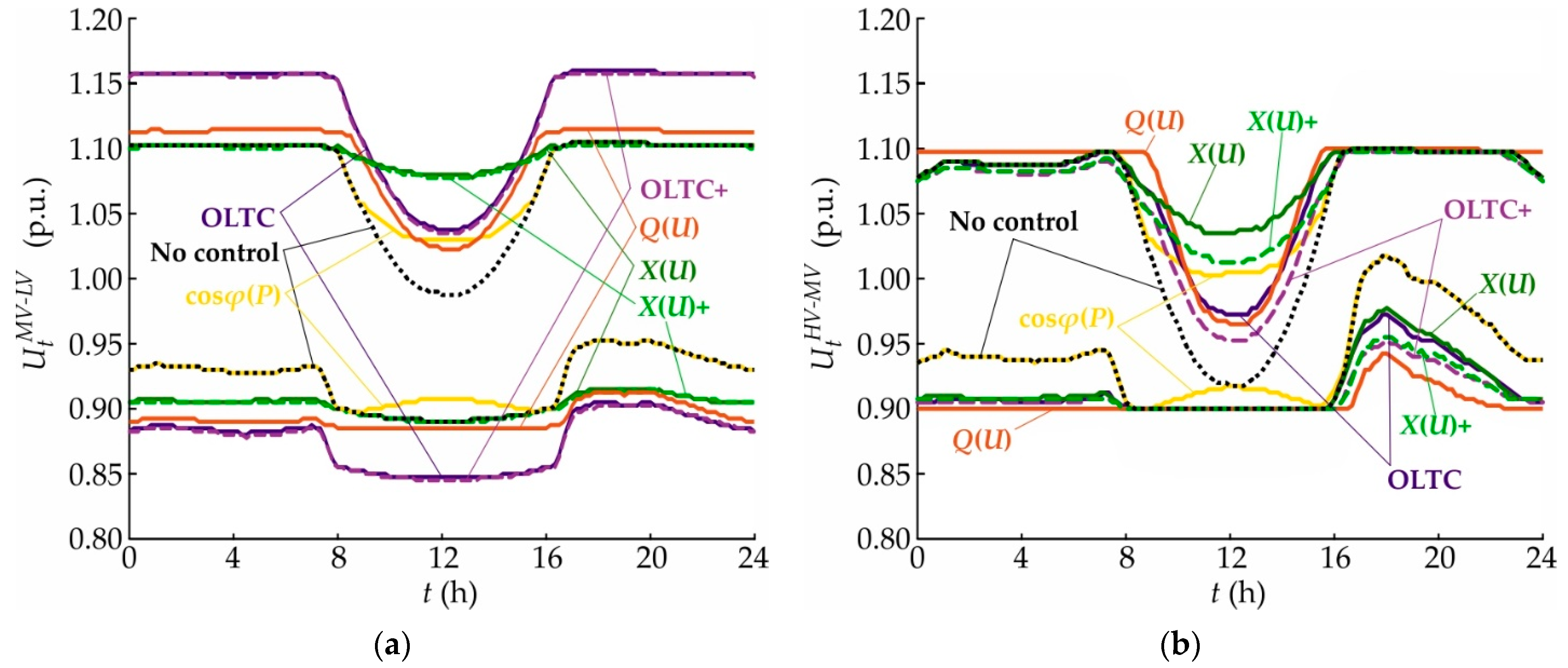
3.1.1. Voltage Behavior
3.1.2. Active Power Exchange
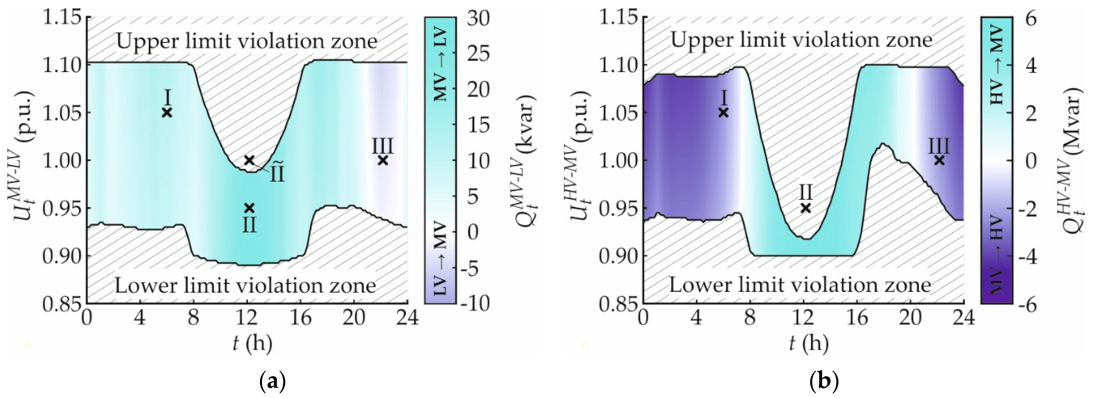
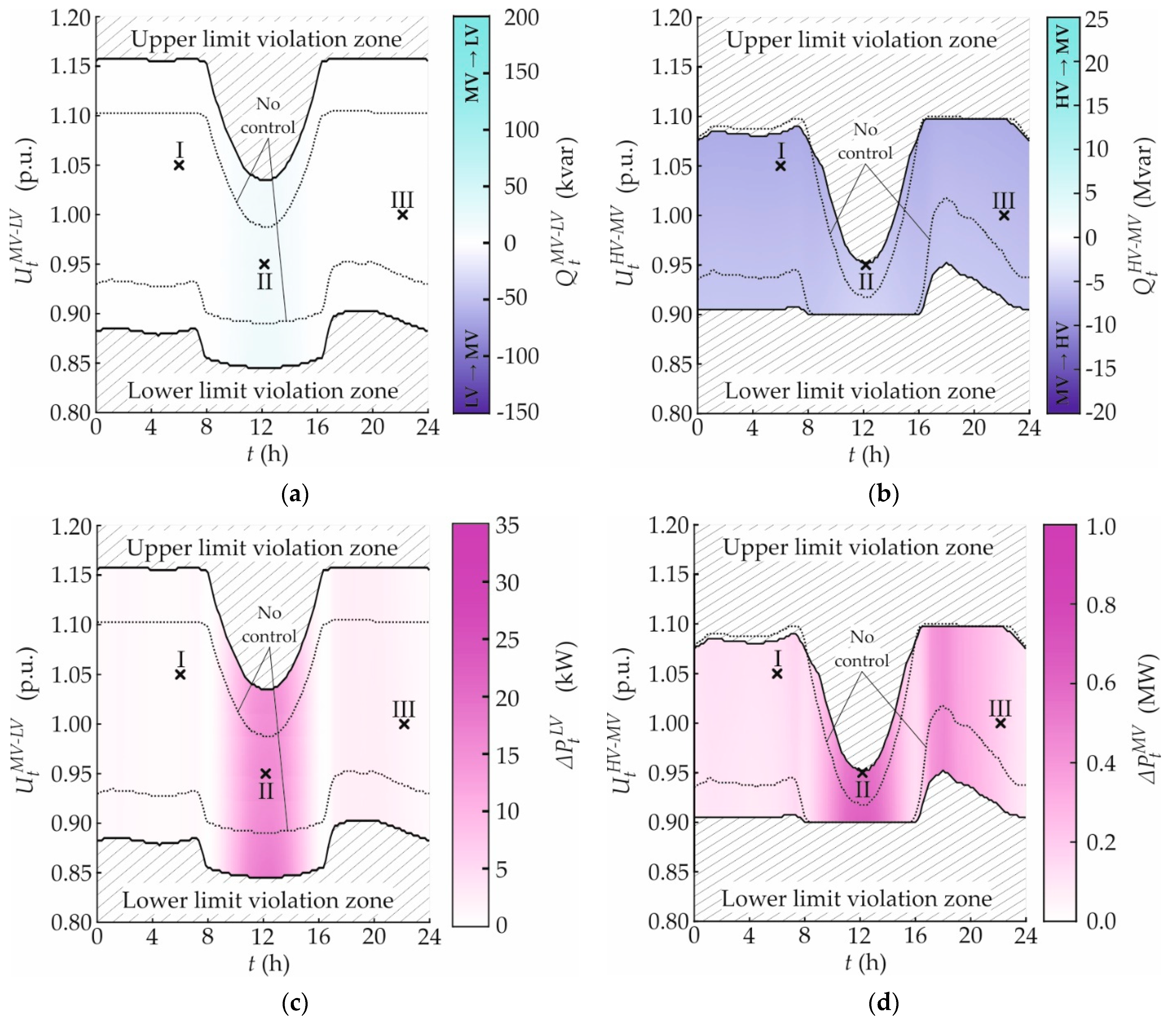
3.1.3. Reactive Power Exchange
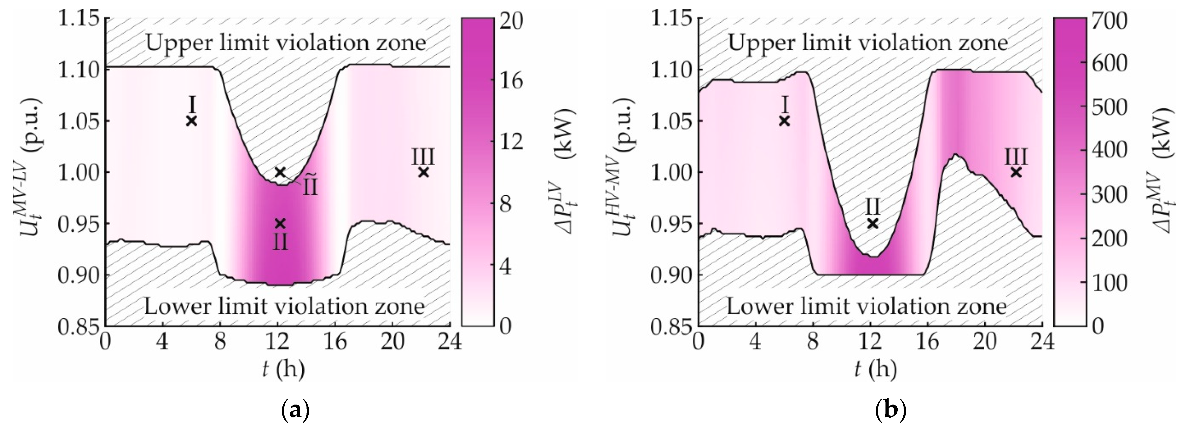
3.1.4. Active Power Loss
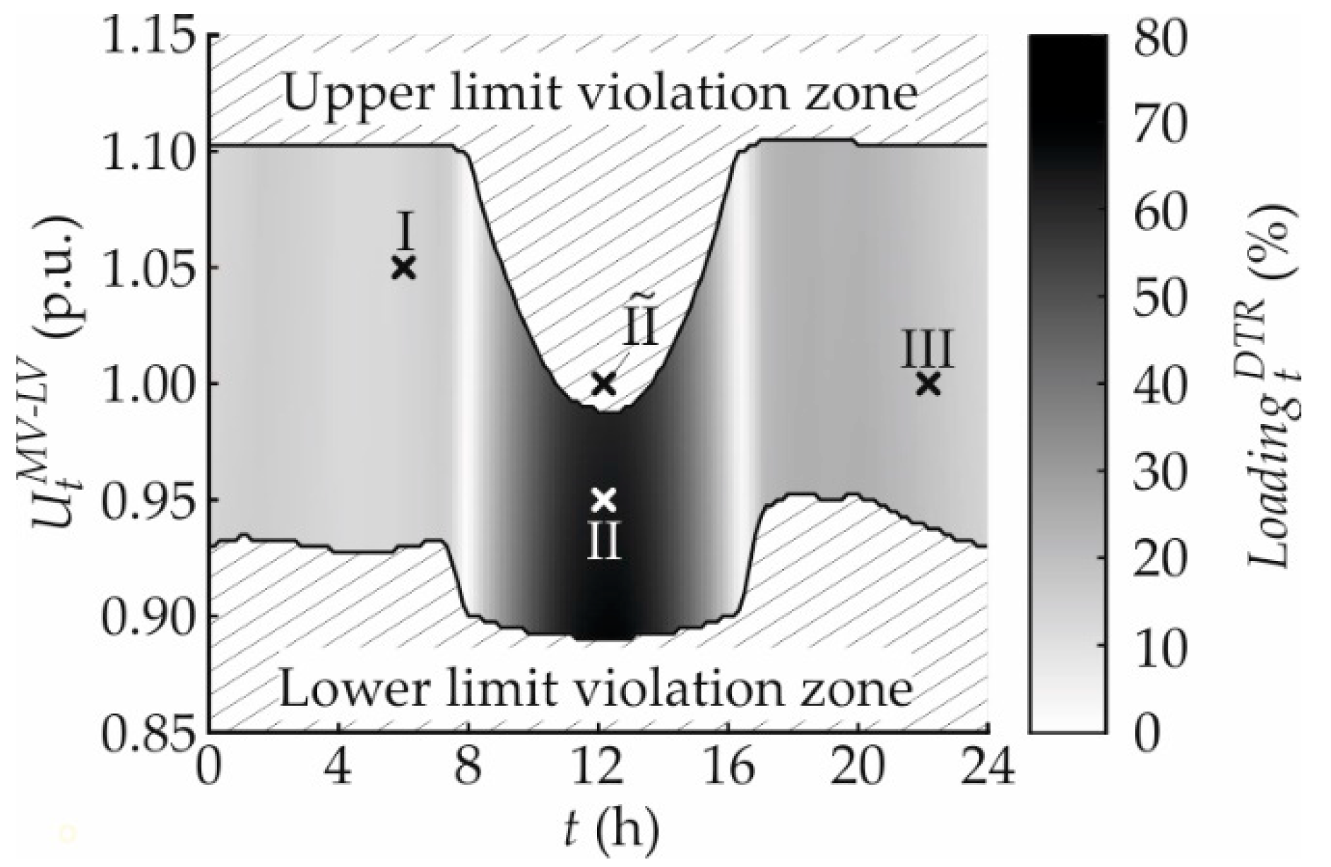
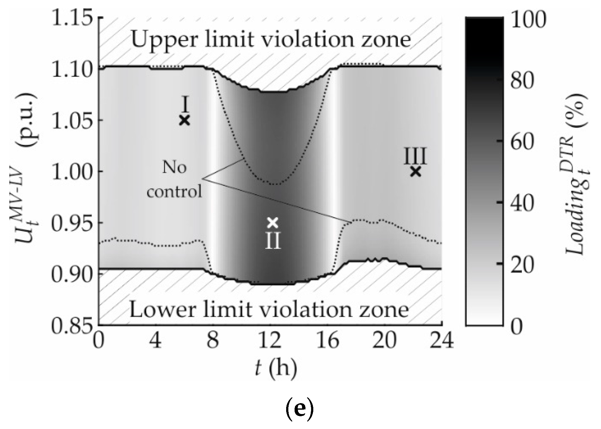
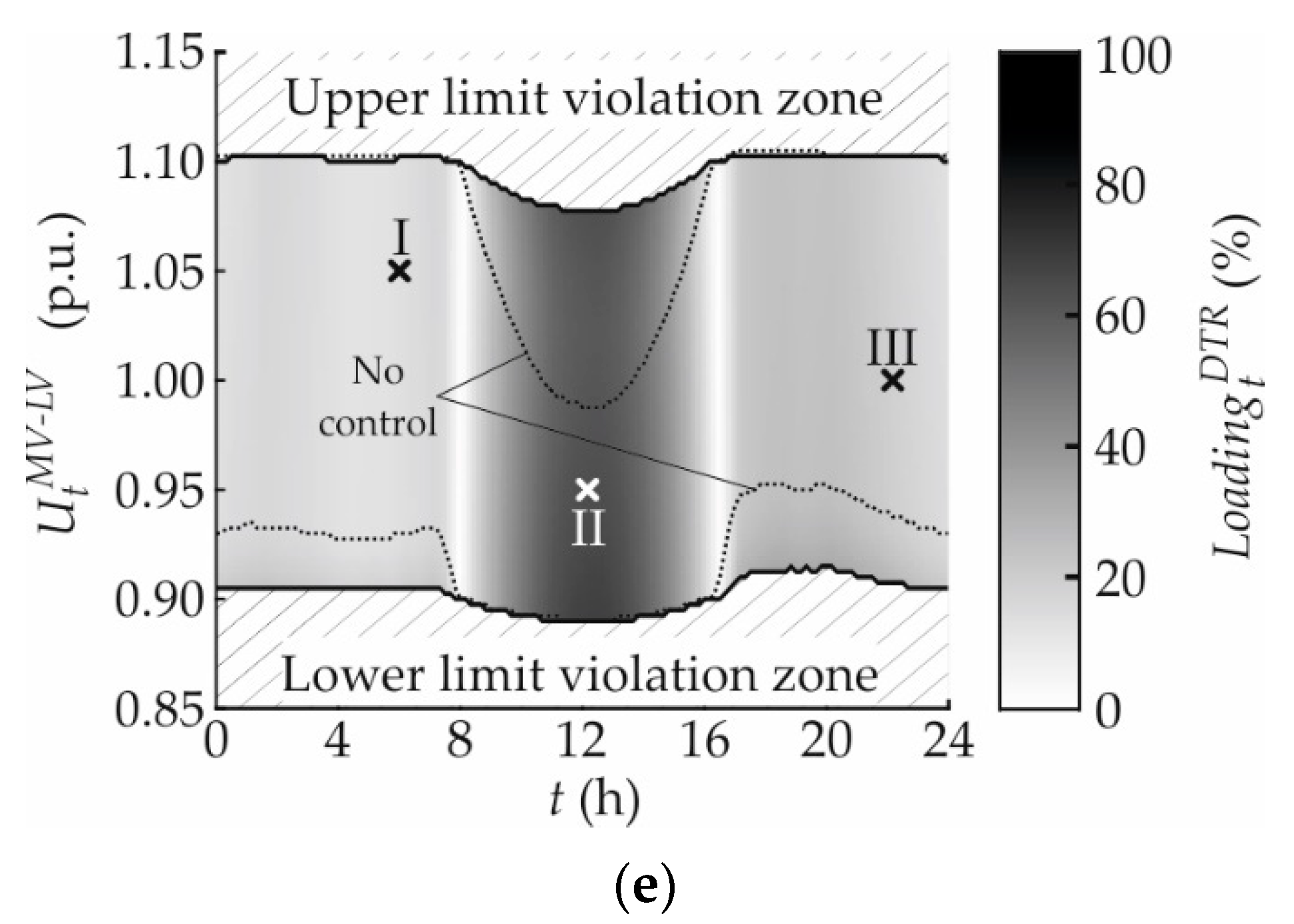
3.1.5. Distribution Transformer Loading
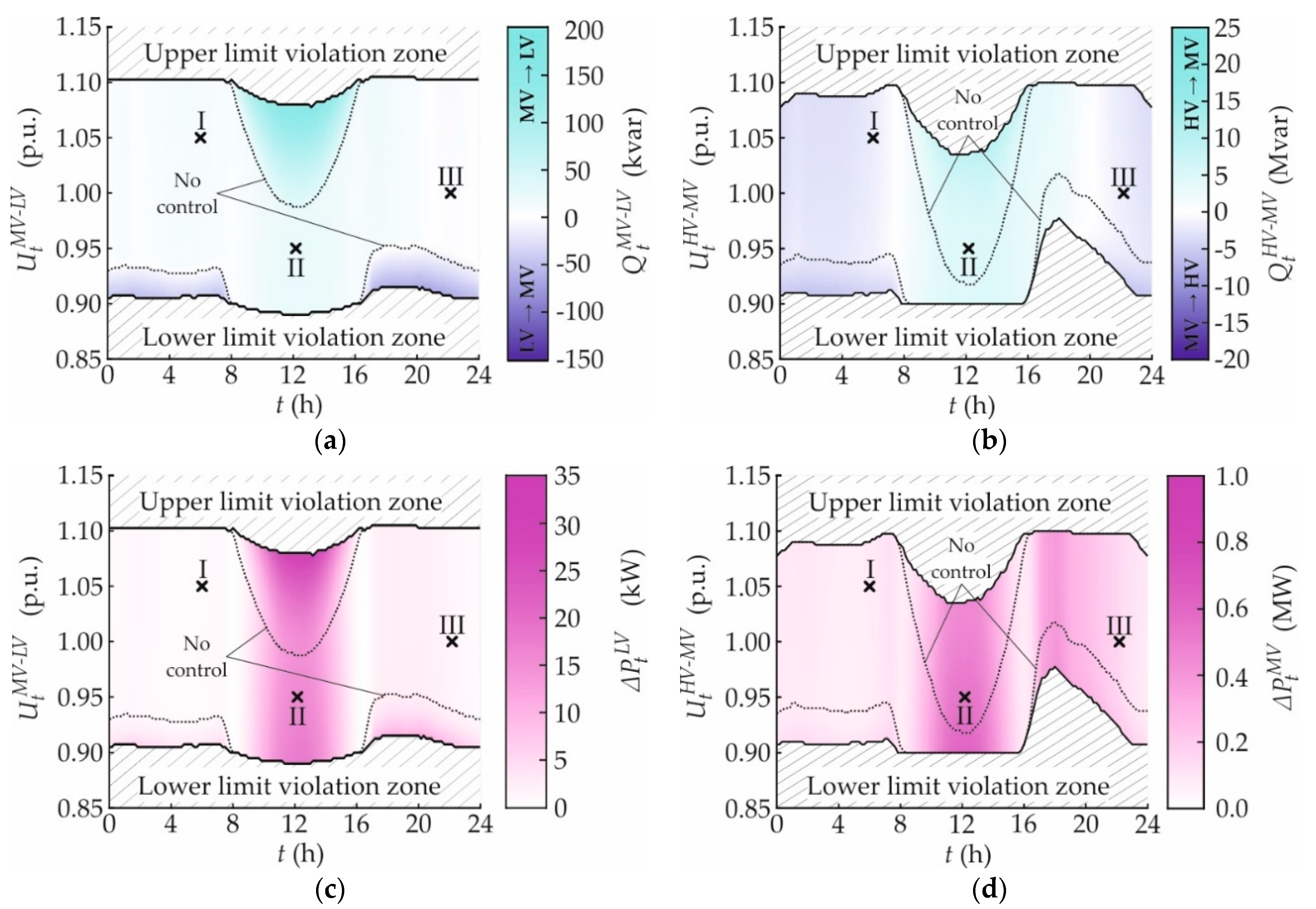
3.2. Local Controls
3.2.1. cosφ(P)
3.2.2. Q(U)
3.2.3. X(U)
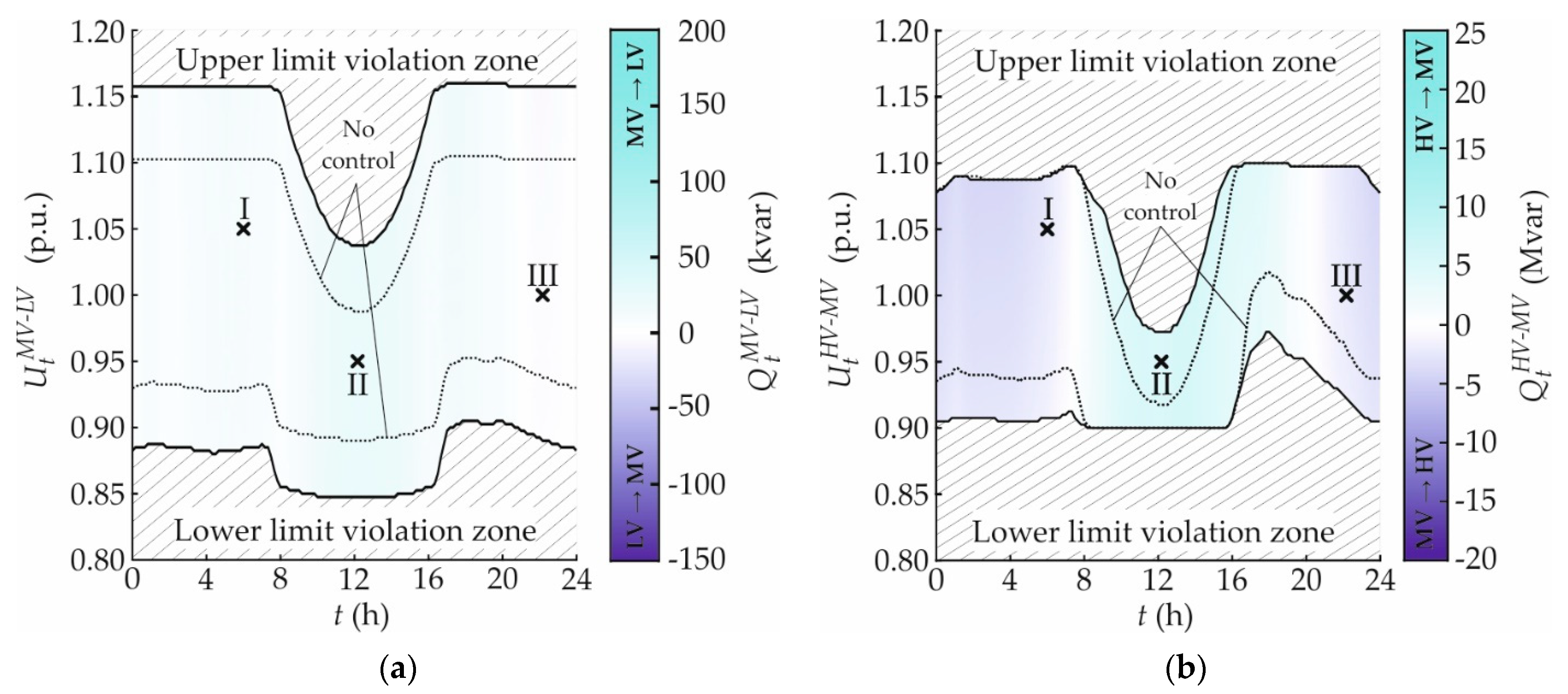
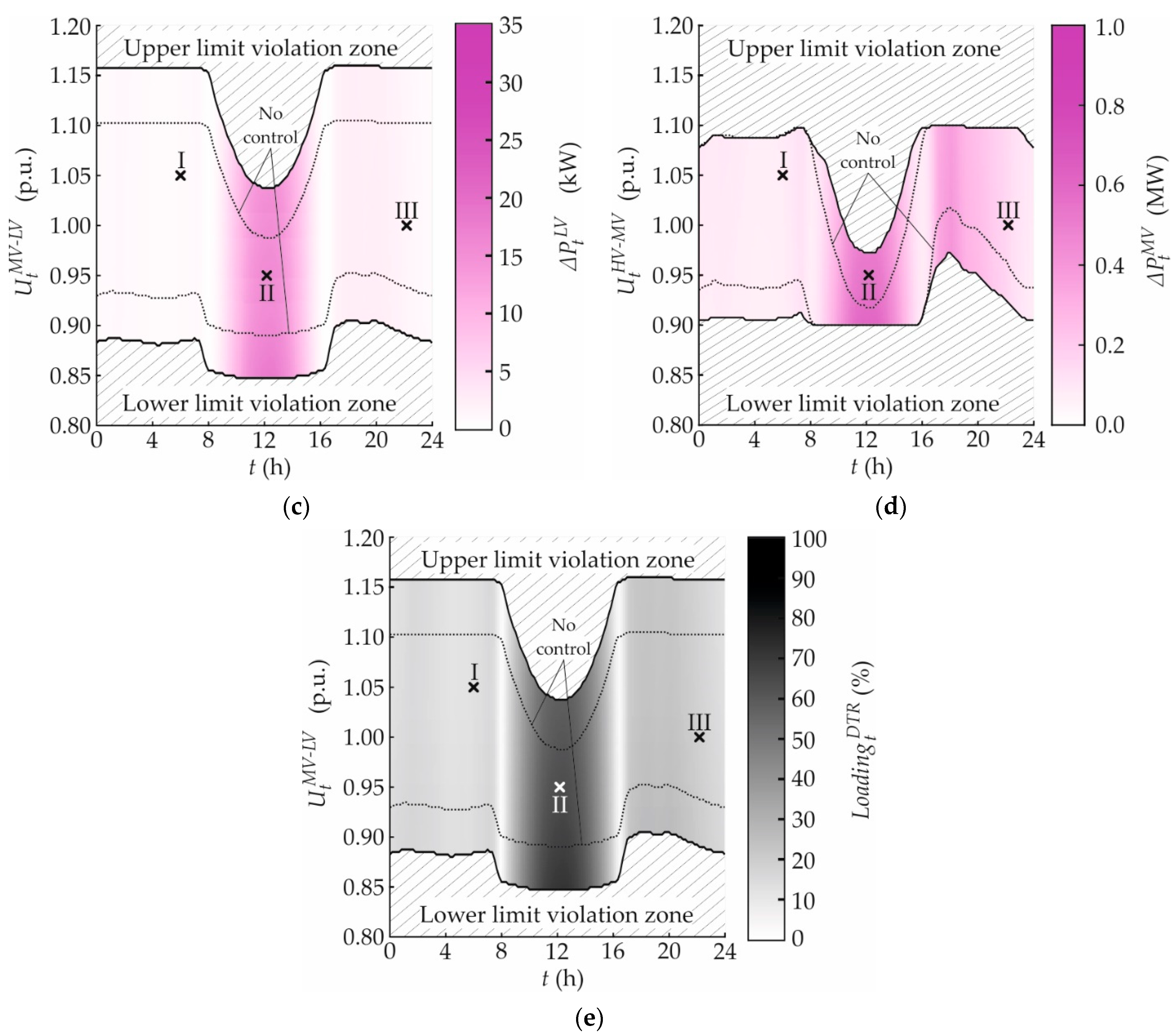
3.2.4. OLTC
3.3. Control Ensembles
3.3.1. X(U) and CP_Q-Autarky
3.3.2. OLTC and CP_Q-Autarky
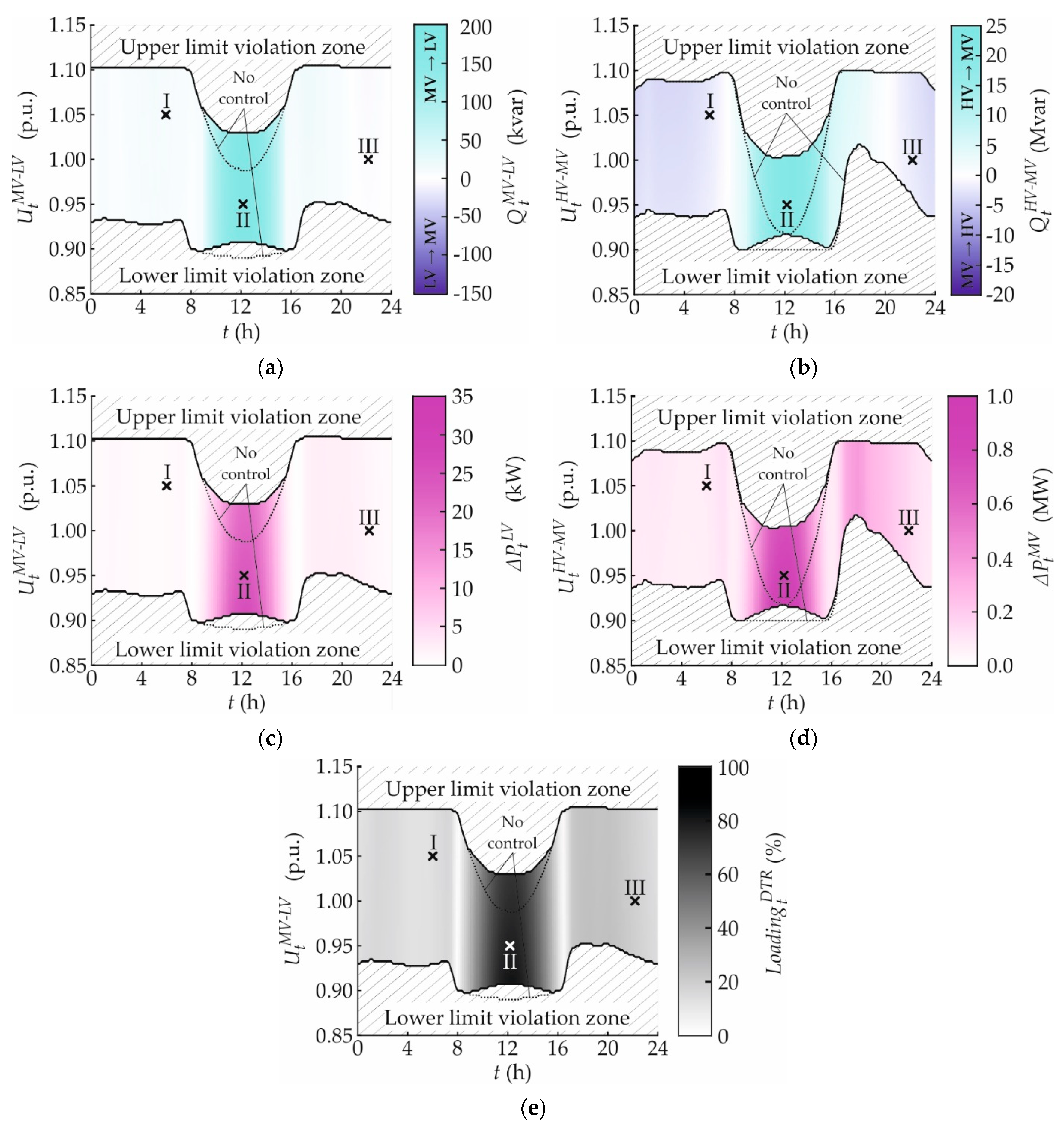
4. Comparison of Volt/var Control Arrangements
4.1. Impact on Boundary Voltage Limits
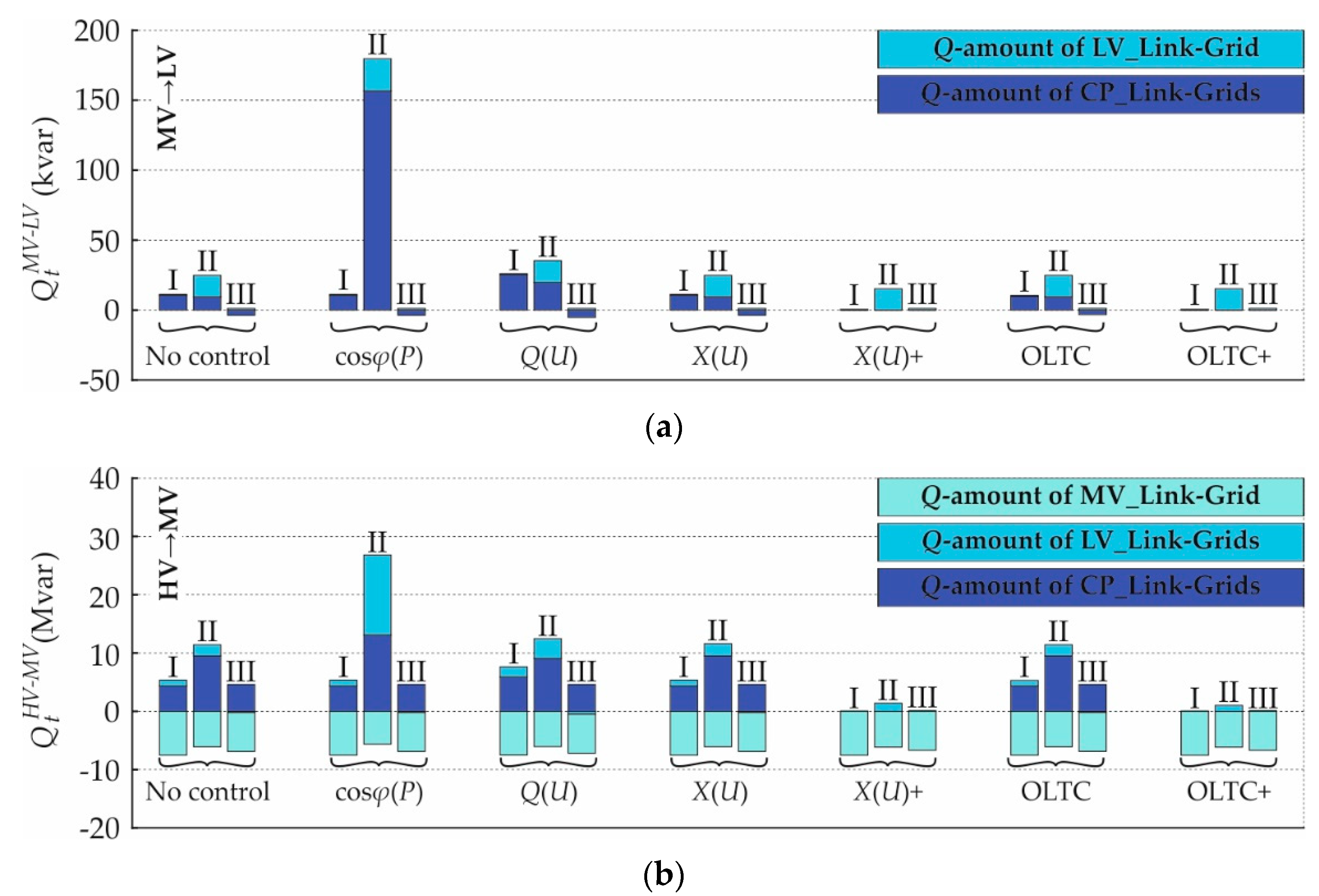
4.2. Impact on Reactive Power Flows
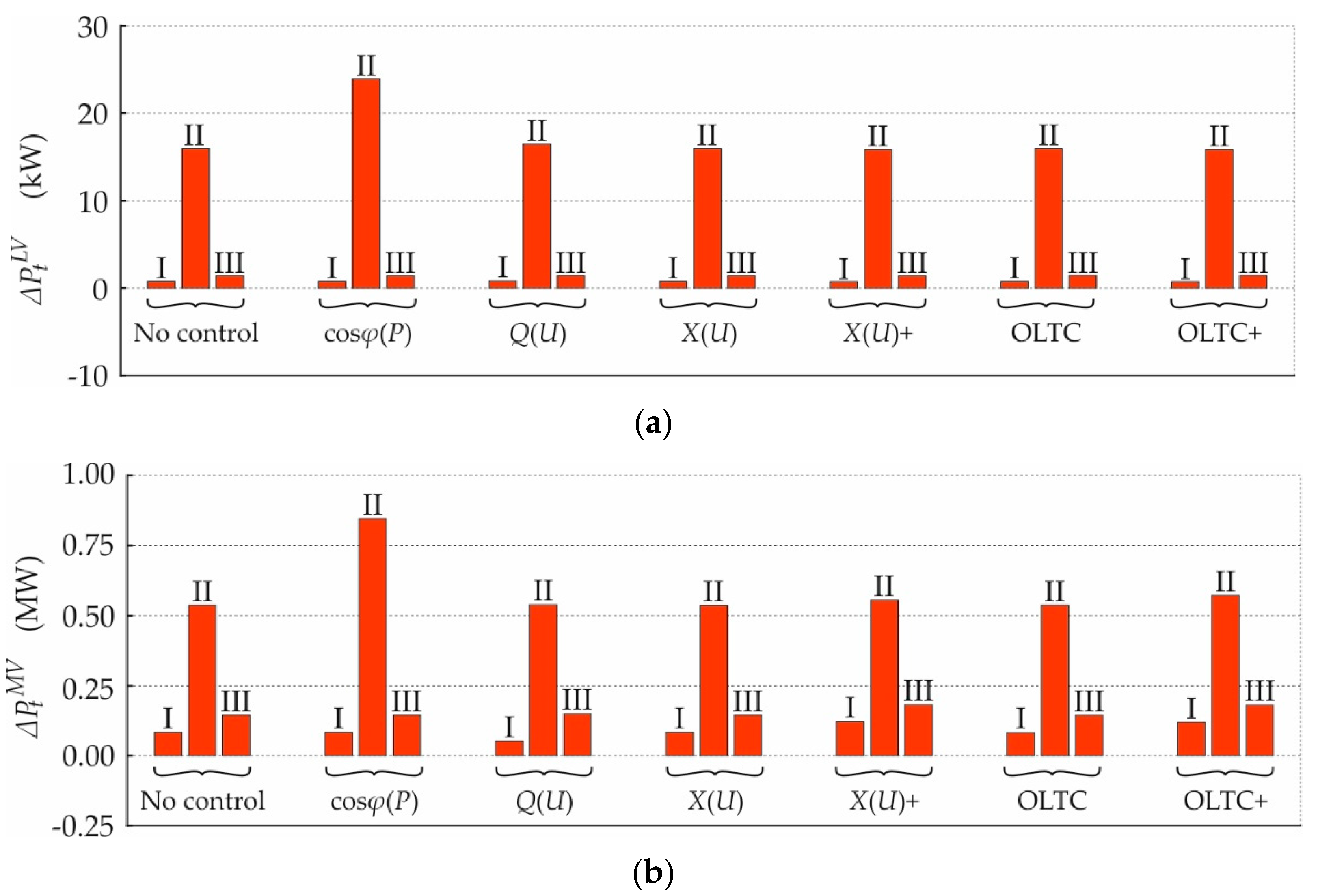
4.3. Impact on Active Power Losses
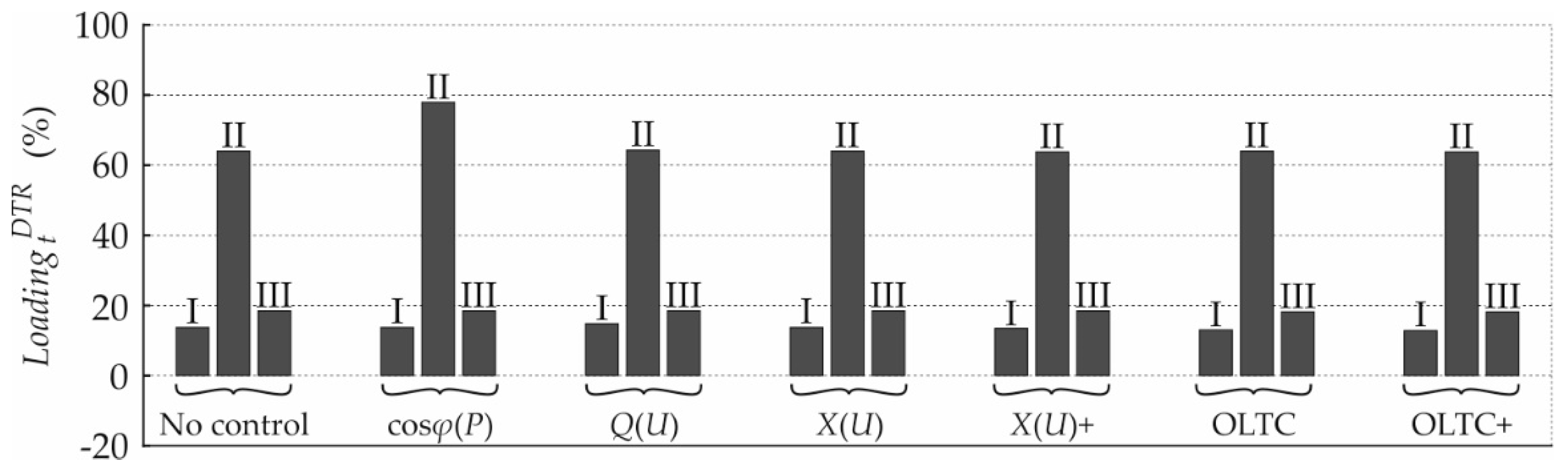
4.4. Impact on Distribution Transformer Loadings
5. Conclusions
Author Contributions
Funding
Data Availability Statement
Conflicts of Interest
Appendix A
- Primary control refers to control actions executed locally in a closed-loop: The input and output variables are the same. The output or control variable is locally measured and continuously compared with the set-point received from the corresponding SC. The deviation from the set-point results in a signal that influences the valves or frequency, excitation current or reactive power, transformer tap positions, etc., in a primary-controlled power plant, transformer, and so on, such that the desired power is delivered or the desired voltage is reached.
- Direct control refers to control actions performed locally in an open-loop, taking into account the holistic real-time behavior of the corresponding grid part. The secondary control calculates the corresponding control action, e.g., changing a circuit breaker’s switch position.
- Secondary control refers to control variables that are calculated based on the current state of a control area. It fulfills a predefined objective function by respecting static and dynamic constraints (P/Q capabilities of generators, transformer and line rating, voltage limits, reactive power limits, etc.). It calculates and sends the set-points to PCs and the input variables DiCs acting on its area.
- Local control refers to control actions that are carried out locally without considering the holistic real-time behavior of the relevant grid part. Its action path may be realized in an open- or closed-loop. LC automatically adjusts the active/reactive power contributions of RPDs, storages, and producers and the tap positions of transformers based on local measurements or time schedules [21,45,46]. It usually maintains a power system parameter, which is locally measured or calculated based on local measurements, equal to the desired value. The fixed control settings are calculated based on offline system analysis for typical operating conditions. LCs are simple, reliable, and respond quickly to changing operating conditions without the need for a communication infrastructure [47,48,49].
Appendix B
- Urban residential CP_Link-Grid
- Commercial CP_Link-Grid

- Industrial CP

References
- Lopes, J.A.P.; Hatziargyriou, N.; Mutale, J.; Djapic, P.; Jenkins, N. Integrating Distributed Generation into Electric Power Systems: A Review of Drivers, Challenges and Opportunities. Electr. Power Syst. Res. 2007, 77, 1189–1203. [Google Scholar] [CrossRef]
- Bollen, M.H.J.; Sannino, A. Voltage Control with Inverter-Based Distributed Generation. IEEE Trans. Power Deliv. 2005, 20, 519–520. [Google Scholar] [CrossRef]
- Bletterie, B.; Kadam, S.; Bolgaryn, R.; Zegers, A. Voltage Control with PV Inverters in Low Voltage Networks—In Depth Analysis of Different Concepts and Parameterization Criteria. IEEE Trans. Power Syst. 2017, 32, 177–185. [Google Scholar] [CrossRef]
- Demirok, E.; González, P.C.; Frederiksen, K.H.B.; Sera, D.; Rodriguez, P.; Teodorescu, R. Local Reactive Power Control Methods for Overvoltage Prevention of Distributed Solar Inverters in Low-Voltage Grids. IEEE J. Photovolt. 2011, 1, 174–182. [Google Scholar] [CrossRef]
- Turitsyn, K.; Sulc, P.; Backhaus, S.; Chertkov, M. Options for Control of Reactive Power by Distributed Photovoltaic Generators. Proc. IEEE 2011, 99, 1063–1073. [Google Scholar] [CrossRef]
- Karthikeyan, N.; Pokhrel, B.R.; Pillai, J.R.; Bak-Jensen, B. Coordinated Voltage Control of Distributed PV Inverters for Voltage Regulation in Low Voltage Distribution Networks. In Proceedings of the 2017 IEEE PES Innovative Smart Grid Technologies Conference Europe (ISGT-Europe), Turin, Italy, 26–29 September 2017; pp. 1–6. [Google Scholar]
- Smith, J.W.; Sunderman, W.; Dugan, R.; Seal, B. Smart Inverter Volt/Var Control Functions for High Penetration of PV on Distribution Systems. In Proceedings of the 2011 IEEE/PES Power Systems Conference and Exposition, Phoenix, AZ, USA, 20–23 March 2011; pp. 1–6. [Google Scholar]
- Zhang, F.; Guo, X.; Chang, X.; Fan, G.; Chen, L.; Wang, Q.; Tang, Y.; Dai, J. The Reactive Power Voltage Control Strategy of PV Systems in Low-Voltage String Lines. In Proceedings of the 2017 IEEE Manchester PowerTech, Manchester, UK, 18–22 June 2017; pp. 1–6. [Google Scholar]
- Wang, J.; Bharati, G.R.; Paudyal, S.; Ceylan, O.; Bhattarai, B.P.; Myers, K.S. Coordinated Electric Vehicle Charging With Reactive Power Support to Distribution Grids. IEEE Trans. Ind. Inform. 2019, 15, 54–63. [Google Scholar] [CrossRef]
- Leemput, N.; Geth, F.; Van Roy, J.; Büscher, J.; Driesen, J. Reactive Power Support in Residential LV Distribution Grids through Electric Vehicle Charging. Sustain. Energy Grids Netw. 2015, 3, 24–35. [Google Scholar] [CrossRef]
- Ilo, A.; Schultis, D.-L.; Schirmer, C. Effectiveness of Distributed vs. Concentrated Volt/Var Local Control Strategies in Low-Voltage Grids. Appl. Sci. 2018, 8, 1382. [Google Scholar] [CrossRef]
- Stetz, T.; Marten, F.; Braun, M. Improved Low Voltage Grid-Integration of Photovoltaic Systems in Germany. IEEE Trans. Sustain. Energy 2013, 4, 534–542. [Google Scholar] [CrossRef]
- Schultis, D.-L.; Ilo, A.; Schirmer, C. Overall Performance Evaluation of Reactive Power Control Strategies in Low Voltage Grids with High Prosumer Share. Electr. Power Syst. Res. 2019, 168, 336–349. [Google Scholar] [CrossRef]
- EU. Regulation (EU) 2016/679 of the European Parliament and of the Council of 27 April 2016 on the Protection of Natural Persons with Regard to the Processing of Personal Data and on the Free Movement of Such Data, and Repealing Directive 95/46/EC (General Data Protection Regulation) (Text with EEA Relevance); EU: Maastricht, The Netherlands, 2016. [Google Scholar]
- EU. Directive (EU) 2019/944 of the European Parliament and of the Council of 5 June 2019 on Common Rules for the Internal Market for Electricity and Amending Directive 2012/27/EU (Text with EEA Relevance.); EU: Maastricht, The Netherlands, 2019. [Google Scholar]
- Reese, C.; Buchhagen, C.; Hofmann, L. Voltage Range as Control Input for OLTC-Equipped Distribution Transformers. In Proceedings of the PES T&D 2012, Orlando, FL, USA, 7–10 May 2012; pp. 1–6. [Google Scholar]
- Hossain, M.I.; Yan, R.; Saha, T. Investigation of the Interaction between Step Voltage Regulators and Large-Scale Photovoltaic Systems Regarding Voltage Regulation and Unbalance. IET Renew. Power Gener. 2016, 10, 299–309. [Google Scholar] [CrossRef]
- Ilo, A.; Schultis, D.-L. Low-Voltage Grid Behaviour in the Presence of Concentrated Var-Sinks and Var-Compensated Customers. Electr. Power Syst. Res. 2019, 171, 54–65. [Google Scholar] [CrossRef]
- Ostergaard, J.; Ziras, C.; Bindner, H.W.; Kazempour, J.; Marinelli, M.; Markussen, P.; Rosted, S.H.; Christensen, J.S. Energy Security Through Demand-Side Flexibility: The Case of Denmark. IEEE Power Energy Mag. 2021, 19, 46–55. [Google Scholar] [CrossRef]
- Chiang, H.-D.; Wang, J.-C.; Tong, J.; Darling, G. Optimal Capacitor Placement, Replacement and Control in Large-Scale Unbalanced Distribution Systems: Modeling and a New Formulation. IEEE Trans. Power Syst. 1995, 10, 356–362. [Google Scholar] [CrossRef]
- Guo, Q.; Qi, J.; Ajjarapu, V.; Bravo, R.; Chow, J.; Li, Z.; Moghe, R.; Nasr-Azadani, E.; Tamrakar, U.; Taranto, G.N.; et al. Review of Challenges and Research Opportunities for Voltage Control in Smart Grids. IEEE Trans. Power Syst. 2019, 34, 2790–2801. [Google Scholar] [CrossRef]
- Lund, P. The Danish Cell Project—Part 1: Background and General Approach. In Proceedings of the 2007 IEEE Power Engineering Society General Meeting, Tampa, FL, USA, 24–28 June 2007. [Google Scholar] [CrossRef]
- European Distribution System Operators for Smart Grids—Data Management: The Role of Distribution System Operators in Managing Data. Available online: https://www.edsoforsmartgrids.eu/wp-content/uploads/public/EDSO-views-on-Data-Management-June-2014.pdf (accessed on 27 August 2021).
- Myrda, P.; Mcgranaghan, M. Smart Grid Enabled Asset Management. In Proceedings of the CIRED Workshop, Lyon, France, 7–8 June 2010; pp. 1–4. [Google Scholar]
- Cárdenas, A.A.; Safavi-Naini, R. Chapter 25—Security and Privacy in the Smart Grid. In Handbook on Securing Cyber-Physical Critical Infrastructure; Das, S.K., Kant, K., Zhang, N., Eds.; Morgan Kaufmann: Boston, MA, USA, 2012; pp. 637–654. ISBN 978-0-12-415815-3. [Google Scholar]
- Vaahedi, E. Practical Power System Operation, 1st ed.; John Wiley & Sons, Ltd.: Hoboken, NJ, USA, 2014. [Google Scholar]
- O’Connell, N.; Pinson, P.; Madsen, H.; O’Malley, M. Benefits and Challenges of Electrical Demand Response: A Critical Review. Renew. Sustain. Energy Rev. 2014, 39, 686–699. [Google Scholar] [CrossRef]
- Ilo, A. “Link”—The Smart Grid Paradigm for a Secure Decentralized Operation Architecture. Electr. Power Syst. Res. 2016, 131, 116–125. [Google Scholar] [CrossRef]
- Schultis, D.-L.; Ilo, A. Behaviour of Distribution Grids with the Highest PV Share Using the Volt/Var Control Chain Strategy. Energies 2019, 12, 3865. [Google Scholar] [CrossRef]
- Ilo, A. The Energy Supply Chain Net. Energy Power Eng. 2013, 5, 384–390. [Google Scholar] [CrossRef][Green Version]
- Luo, K.; Shi, W. Comparison of Voltage Control by Inverters for Improving the PV Penetration in Low Voltage Networks. IEEE Access 2020, 8, 161488–161497. [Google Scholar] [CrossRef]
- Almeida, D.; Pasupuleti, J.; Ekanayake, J. Comparison of Reactive Power Control Techniques for Solar PV Inverters to Mitigate Voltage Rise in Low-Voltage Grids. Electronics 2021, 10, 1569. [Google Scholar] [CrossRef]
- Chathurangi, D.; Jayatunga, U.; Perera, S.; Agalgaonkar, A.P.; Siyambalapitiya, T. Comparative Evaluation of Solar PV Hosting Capacity Enhancement Using Volt-VAr and Volt-Watt Control Strategies. Renew. Energy 2021, 177, 1063–1075. [Google Scholar] [CrossRef]
- Schultis, D.-L. Comparison of Local Volt/Var Control Strategies for PV Hosting Capacity Enhancement of Low Voltage Feeders. Energies 2019, 12, 1560. [Google Scholar] [CrossRef]
- Schultis, D.-L.; Ilo, A. Increasing the Utilization of Existing Infrastructures by Using the Newly Introduced Boundary Voltage Limits. Energies 2021, 14, 5106. [Google Scholar] [CrossRef]
- DIN EN 50160:2020-11, Merkmale Der Spannung in Öffentlichen Elektrizitätsversorgungsnetzen; Deutsche Fassung EN_50160:2010_+ Cor.: 2010_+ A1:2015_+ A2:2019_+ A3:2019; Beuth Verlag GmbH: Berlin, Germany, 2020.
- Schultis, D.-L. Daily Load Profiles and ZIP Models of Current and New Residential Customers; Data Archiving and Networked Services (DANS): Den Haag, The Netherlands, 2019; Volume 1. [Google Scholar] [CrossRef]
- Schultis, D.-L.; Ilo, A. Adaption of the Current Load Model to Consider Residential Customers Having Turned to LED Lighting. In Proceedings of the 2019 IEEE PES Asia-Pacific Power and Energy Engineering Conference (APPEEC), Macao, China, 1–4 December 2019; pp. 1–5. [Google Scholar]
- Wang, Y.-B.; Wu, C.-S.; Liao, H.; Xu, H.-H. Steady-State Model and Power Flow Analysis of Grid-Connected Photovoltaic Power System. In Proceedings of the 2008 IEEE International Conference on Industrial Technology, Chengdu, China, 21–24 April 2008; pp. 1–6. [Google Scholar]
- Shukla, A.; Verma, K.; Kumar, R. Multi-Stage Voltage Dependent Load Modelling of Fast Charging Electric Vehicle. In Proceedings of the 2017 6th International Conference on Computer Applications In Electrical Engineering-Recent Advances (CERA), Roorkee, India, 5–7 October 2017; pp. 86–91. [Google Scholar]
- Aunedi, M.; Woolf, M.; Strbac, G.; Babalola, O.; Clark, M. Characteristic Demand Profiles of Residential and Commercial EV Users and Opportunities for Smart Charging. In Proceedings of the 23rd International Conference on Electricity Distribution (CIRED 2015), Lyon, France, 15–18 June 2015; pp. 1–5. [Google Scholar]
- Schultis, D.-L.; Ilo, A. TUWien_LV_TestGrids; Mendeley Data: London, UK, 2018; Volume 1. [Google Scholar] [CrossRef]
- Technische und Organisatorische Regeln für Betreiber und Benutzer von Netzen. TOR Erzeuger: Anschluss und Parallelbetrieb von Stromerzeugungsanlagen des Typs A und von Kleinsterzeugungsanlagen. Available online: https://www.e-control.at/documents/1785851/1811582/TOR+Erzeuger+Typ+A+V1.0.pdf/6342d021-a5ce-3809-2ae5-28b78e26f04d?t=1562757767659 (accessed on 27 July 2021).
- Marggraf, O.; Laudahn, S.; Engel, B.; Lindner, M.; Aigner, C.; Witzmann, R.; Schoeneberger, M.; Patzack, S.; Vennegeerts, H.; Cremer, M.; et al. U-Control-Analysis of Distributed and Automated Voltage Control in Current and Future Distribution Grids. In Proceedings of the International ETG Congress 2017, Bonn, Germany, 28–29 November 2017; pp. 1–6. [Google Scholar]
- Roytelman, I.; Ganesan, V. Modeling of Local Controllers in Distribution Network Applications. In Proceedings of the 21st International Conference on Power Industry Computer Applications. Connecting Utilities. PICA 99. To the Millennium and Beyond (Cat. No.99CH36351), Santa Clara, CA, USA, 21 May 1999; pp. 161–166. [Google Scholar]
- Farivar, M.; Zho, X.; Chen, L. Local Voltage Control in Distribution Systems: An Incremental Control Algorithm. In Proceedings of the 2015 IEEE International Conference on Smart Grid Communications (SmartGridComm), Miami, FL, USA, 2–5 November 2015; pp. 732–737. [Google Scholar]
- Nowak, S.; Wang, L.; Metcalfe, M.S. Two-Level Centralized and Local Voltage Control in Distribution Systems Mitigating Effects of Highly Intermittent Renewable Generation. Int. J. Electr. Power Energy Syst. 2020, 119, 105858. [Google Scholar] [CrossRef]
- Zhou, X.; Chen, L.; Farivar, M.; Liu, Z.; Low, S. Reverse and Forward Engineering of Local Voltage Control in Distribution Networks. IEEE Trans. Autom. Control 2020, 66, 1116–1128. [Google Scholar] [CrossRef]
- Roytelman, I.; Ganesan, V. Coordinated Local and Centralized Control in Distribution Management Systems. IEEE Trans. Power Deliv. 2000, 15, 718–724. [Google Scholar] [CrossRef]
- Benchmark Systems for Network Integration of Renewable and Distributed Energy Resources. Available online: https://e-cigre.org/publication/ELT_273_8-benchmark-systems-for-network-integration-of-renewable-and-distributed-energy-resources (accessed on 26 July 2021).
- Bokhari, A.; Alkan, A.; Dogan, R.; Diaz-Aguiló, M.; de León, F.; Czarkowski, D.; Zabar, Z.; Birenbaum, L.; Noel, A.; Uosef, R.E. Experimental Determination of the ZIP Coefficients for Modern Residential, Commercial, and Industrial Loads. IEEE Trans. Power Deliv. 2014, 29, 1372–1381. [Google Scholar] [CrossRef]


| LV_Link-Grid | Umin | Umax |
|---|---|---|
| Rural | 0.950 p.u. | 0.990 p.u. |
| Urban | 0.950 p.u. | 1.025 p.u. |
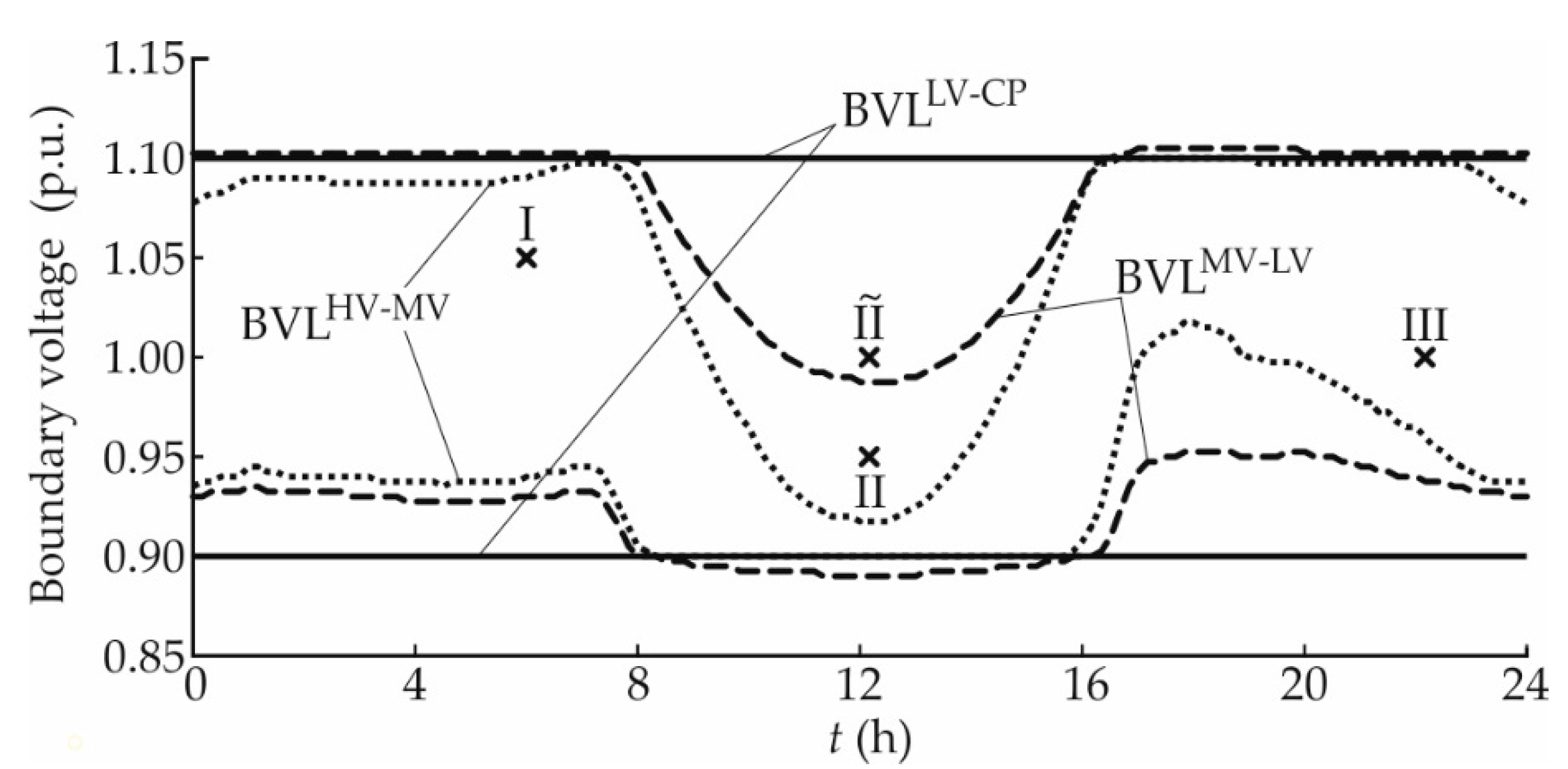
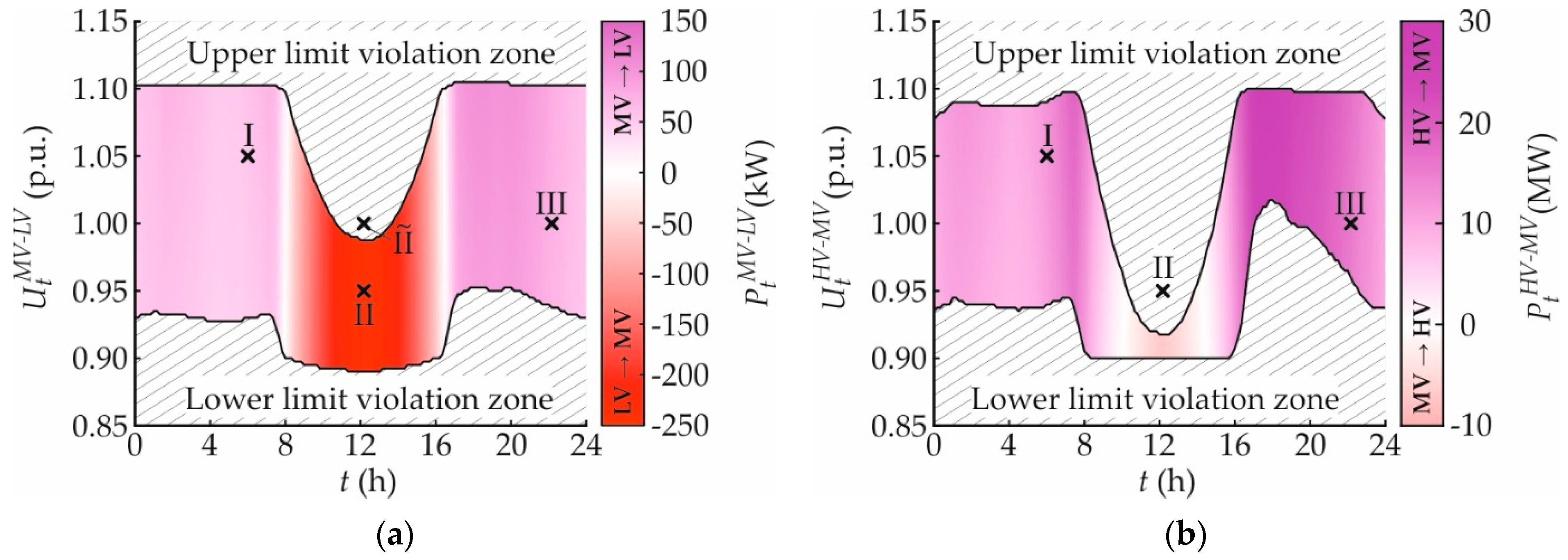
| Case | Boundary Voltage | Daytime |
|---|---|---|
| I | 1.05 p.u. | 06:00 |
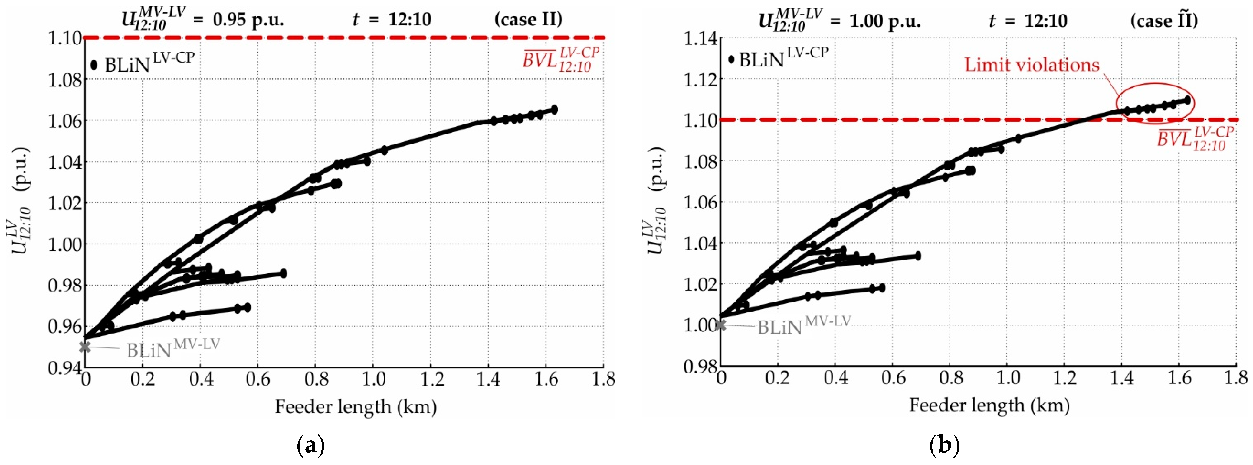
| II | 0.95 p.u. | 12:10 |
| 1.00 p.u. | 12:10 | |
| III | 1.00 p.u. | 22:10 |
| Volt/var Control Arrangement | Voltage Limit Distortion | ||
|---|---|---|---|
| MV−LV Boundary | HV−MV Boundary | Total | |
| No control | 0.1337% | 0.2370% | 0.3707% |
| cosφ(P) local control | 0.1059% | 0.1884% | 0.2943% |
| Q(U) local control | 0.0920% | 0.1233% | 0.2153% |
| X(U) local control | 0.0469% | 0.1233% | 0.1702% |
| X(U) local control and CP_Q-Autarky | 0.0417% | 0.1181% | 0.1598% |
| OLTC local control | 0.1354% | 0.1528% | 0.2882% |
| OLTC local control and CP_Q-Autarky | 0.1354% | 0.1615% | 0.2969% |
Publisher’s Note: MDPI stays neutral with regard to jurisdictional claims in published maps and institutional affiliations. |
© 2021 by the authors. Licensee MDPI, Basel, Switzerland. This article is an open access article distributed under the terms and conditions of the Creative Commons Attribution (CC BY) license (https://creativecommons.org/licenses/by/4.0/).
Share and Cite
Schultis, D.-L.; Ilo, A. Effect of Individual Volt/var Control Strategies in LINK-Based Smart Grids with a High Photovoltaic Share. Energies 2021, 14, 5641. https://doi.org/10.3390/en14185641
Schultis D-L, Ilo A. Effect of Individual Volt/var Control Strategies in LINK-Based Smart Grids with a High Photovoltaic Share. Energies. 2021; 14(18):5641. https://doi.org/10.3390/en14185641
Chicago/Turabian StyleSchultis, Daniel-Leon, and Albana Ilo. 2021. "Effect of Individual Volt/var Control Strategies in LINK-Based Smart Grids with a High Photovoltaic Share" Energies 14, no. 18: 5641. https://doi.org/10.3390/en14185641
APA StyleSchultis, D.-L., & Ilo, A. (2021). Effect of Individual Volt/var Control Strategies in LINK-Based Smart Grids with a High Photovoltaic Share. Energies, 14(18), 5641. https://doi.org/10.3390/en14185641