Online Parameter Estimation for Fault Identification in Multi-Terminal DC Distribution Grids

Abstract

Fast and accurate identification of short-circuit faults is important for post-fault service restoration and maintenance in DC distribution grids. Yet multiple power sources and complex system topologies complicate the fault identification in multi-terminal DC distribution grids. To address this challenge, this paper introduces an approach that achieves fast online identification of both the location and the severity of faults in multi-terminal DC distribution grids. First, a generic model describing the dynamic response of DC lines to both pole-to-ground and pole-to-pole faults with fault currents injected from both line ends is developed. On this basis, a Kalman filter is adopted to estimate both the fault location and resistance. In the real-time simulation of various fault scenarios in a three-terminal DC distribution grid model with Opal-RT platform, the proposed method is proved to be effective with a short response time of less than 1 ms.

1. Introduction

Conventional power systems are undergoing a profound transition led by emerging DC technologies. The far-reaching changes started from the power transmission section, where high-voltage DC (HVDC) systems have been implemented to transmit electric energy over a long distance, and now reach the medium- and low-voltage power distribution levels. Compared with AC grids, DC distribution grids have multiple advantages in terms of efficiency, flexibility and capacity in the integration of distributed renewable energies, energy storage systems and power electronic devices [1,2].

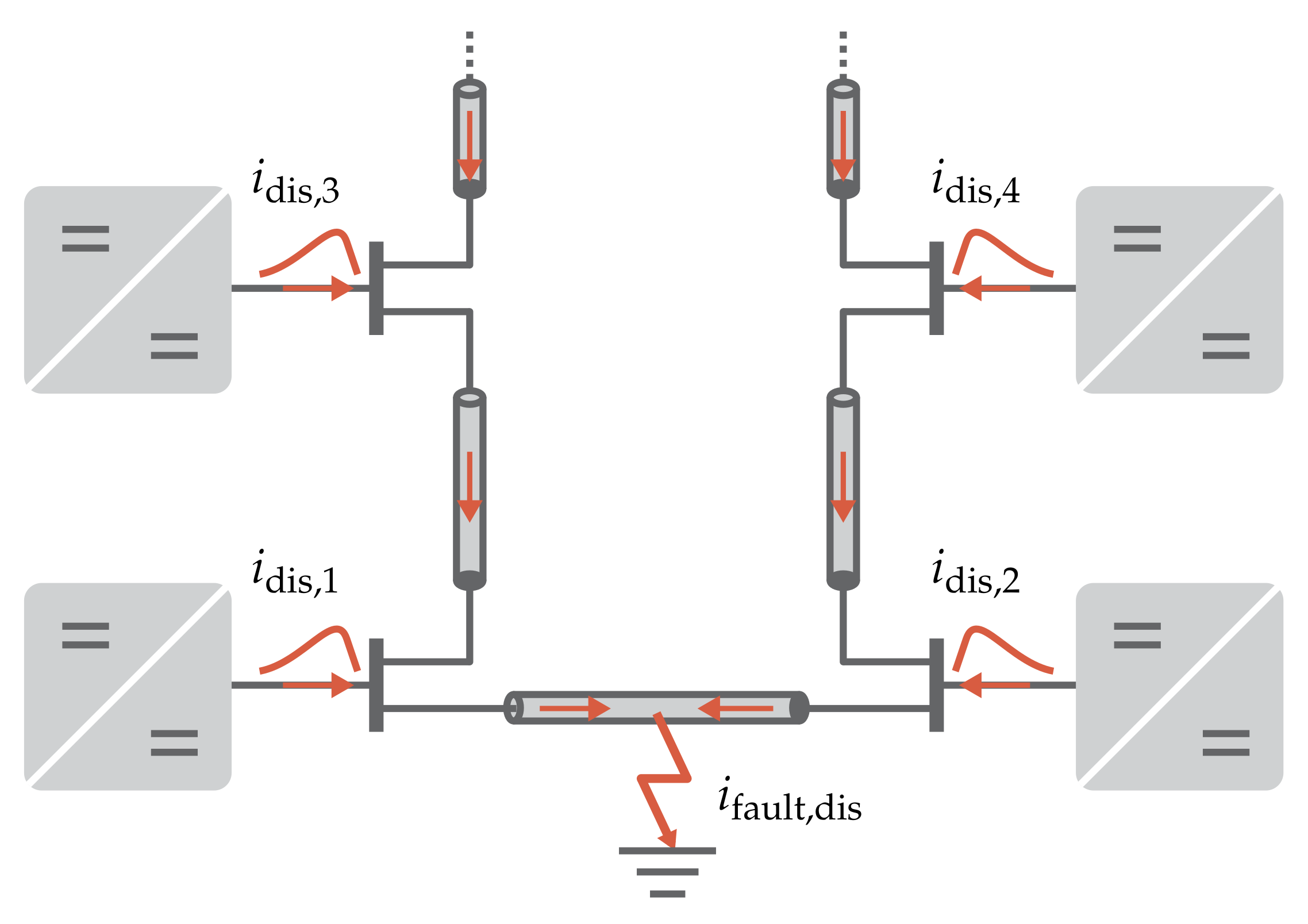
However, short-circuit faults are still a major threat to the safety of multi-terminal DC (MTDC) distribution grids. Because of the low-impedance nature of DC systems, the ensuing fault currents in DC distribution grids increase at high rates, which can damage vulnerable power electronic devices in a few milliseconds [3]. Besides, the multiple power sources and capacitive components in MTDC distribution grids get simultaneously discharged by faults, leading to significant impacts in a large area. To avoid the irreversible damages to the system, it is critical to clear the faults in MTDC distribution grids in the early phase.

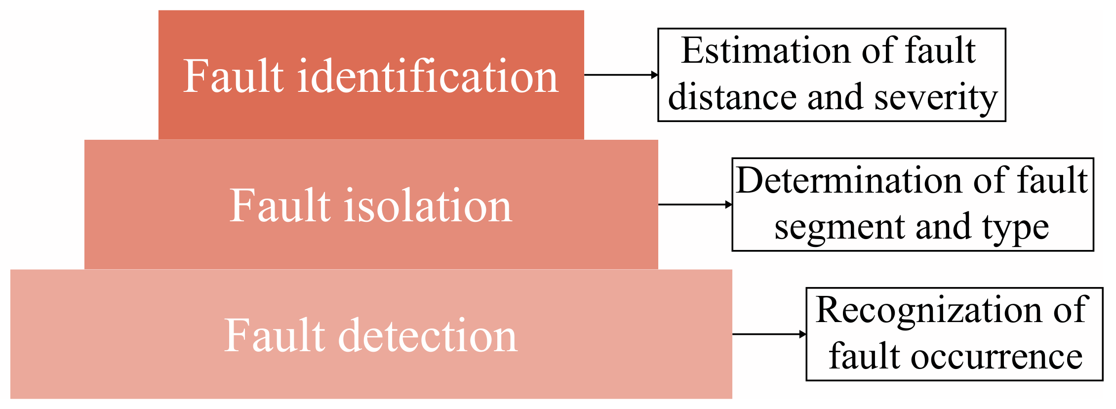
As shown in Figure 1, the fault diagnosis in MTDC distribution grids includes three different levels [4]: fault detection, isolation and identification. Among the three levels, fault detection and isolation are the precondition to achieve selective fault clearance in MTDC distribution grids. Based on the output of fault isolation, fault identification is performed on the recognized fault segments to further obtain quantified fault information. Fault identification is of great importance for the maintenance and service restoration of MTDC distribution grids, which is the focus of this paper. Owning to the need for fast fault clearance in MTDC distribution grids, limited time and data are available for online fault identification, which form the major challenges to existing techniques. The existing online fault identification methods in MTDC distribution grids can be categorized into signal-based, data-based and model-based methods, which are reviewed in the following.

The signal-based methods rely on the processing of real-time measurement signals. There are traveling waves, which can be classified into single-ended type [5] and double-ended type [6]. To improve the accuracy in measuring the time delay of traveling waves, time-frequency analysis techniques, such as wavelet transform [7], have also been used. The traveling wave-based methods are primarily applied to the systems with long transmission distance. However, MTDC distribution grids are in general small-scale networks with short feeder lines. In such systems, the time delays of traveling waves are difficult to measure. Besides, fault location is also achieved through estimating line impedance. An impedance estimation-based fault identification method is introduced in [8]. Yet this method has been tested only in a passive radial DC grid, whereas the impedance of MTDC distribution grids is still difficult to measure. Dedicated power hardware and devices have also been used to aid the fault identification in DC grids [9,10,11]. The active impedance estimation method [9] measures the bus impedance in high-frequency domain using additional power converters.Ref. [10] introduces a fault location module composed of switches and inductors. Ref. [11] injects signals into isolated faulty lines with specialized solid-state circuit breakers. However, due to the needs for additional hardware, these methods are not optimal solutions from the view point of cost and reliability.

The data-based methods achieve fault identification based on the correlation between real-time measurement data and historical data. In this field, supervised machine learning methods have gained more and more attentions. For example, ref. [12] trains artificial neural networks to locate faults in DC microgrids, ref. [13] implements a fault location function in photovoltaic farms with artificial neural networks and wavelet transform, ref. [14] introduces the support vector machine for fault classification and identification in DC lines. In [15], pre-simulated fault data are used as the training samples to train a machine learning model for fault location. The general problem of these supervised machine learning methods is that their performances are highly dependent on the availability of labeled training data, especially fault data, which are difficult to acquire and only sparsely available in real-world power systems. As for those models trained with simulation data, their effectiveness in realistic fault conditions is not verified.

Moreover, the dynamic models of DC cables have been used for fault identification in DC distribution grids. Based on this concept, different methods have been proposed. For example, ref. [16] estimates the fault distance and location in DC microgrids using the signals measured during fault transients. Yet this method uses the derivatives of line currents, whose accuracy is highly susceptible to noises and sampling errors. Ref. [17] develops a non-iterative algorithm to estimate the fault distance based on the discrete equations of differential currents. However, the computational costs of this method increase with the length of cable. Ref. [18] provides a parameter estimation approach to estimate both fault location and resistance. Yet the accuracy and speed of this local measurement-based method are still to improve. Ref. [19] introduces a genetic algorithm-based fault location method in DC distribution grids. However, the estimation of fault severity is not covered. Ref. [20] establishes a R-L model of DC lines for fault location. However, the requirement of preset short-circuit faults contribute to the difficulty in the implementation of this method. Ref. [21] estimates fault distance based on a voltage divider in DC lines, which contributes to installation costs.

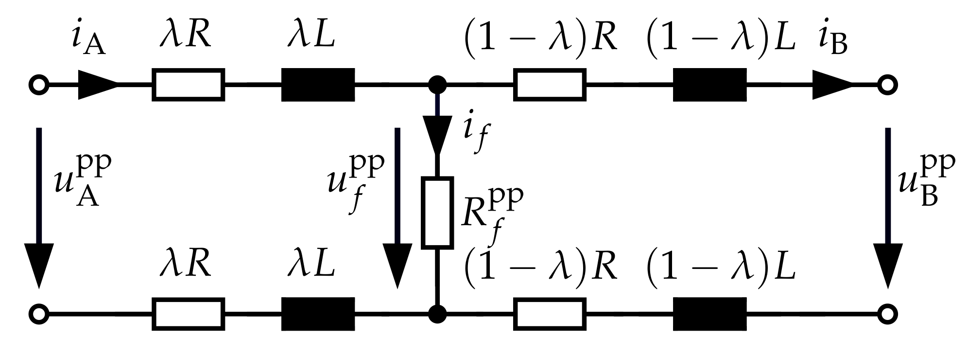
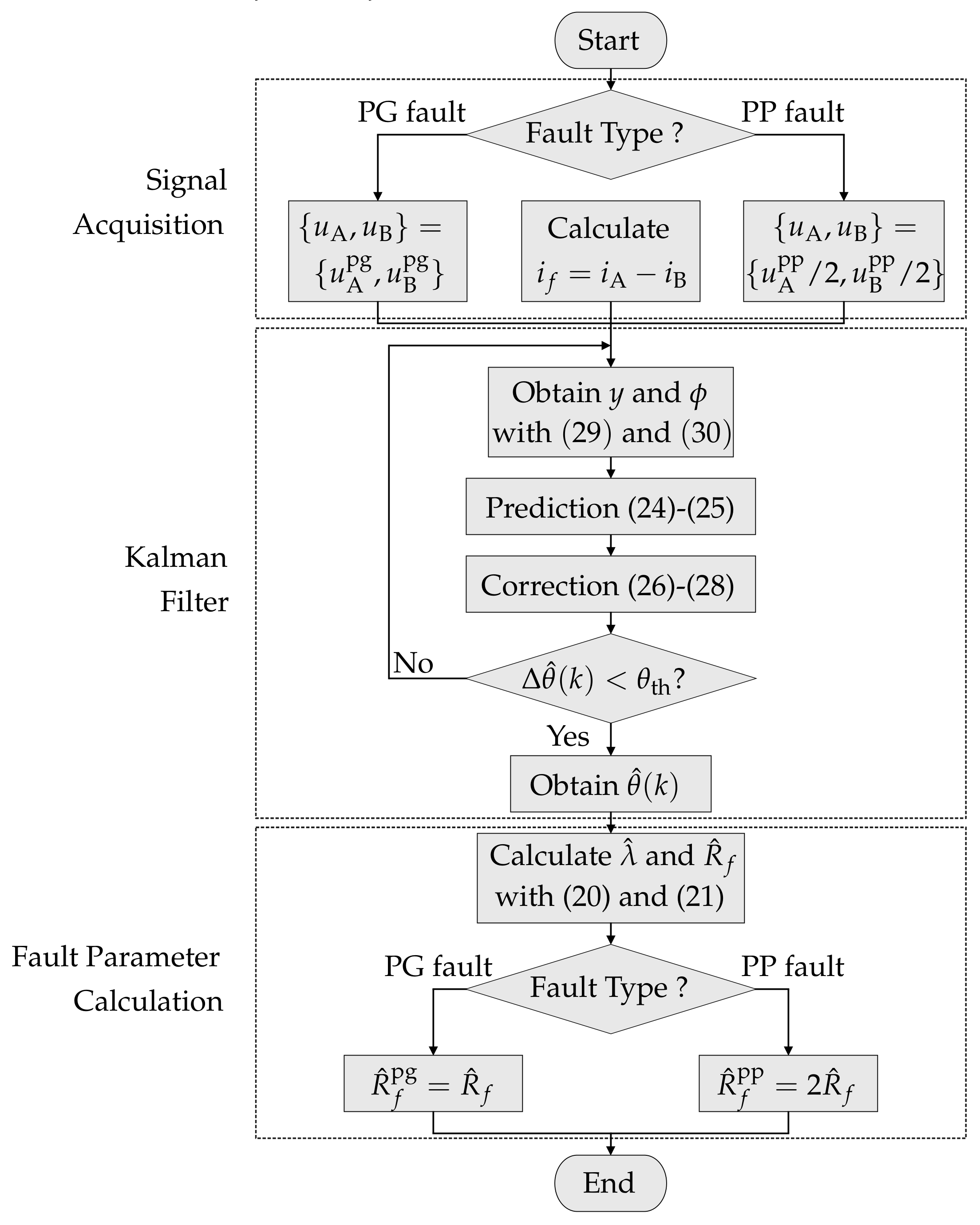
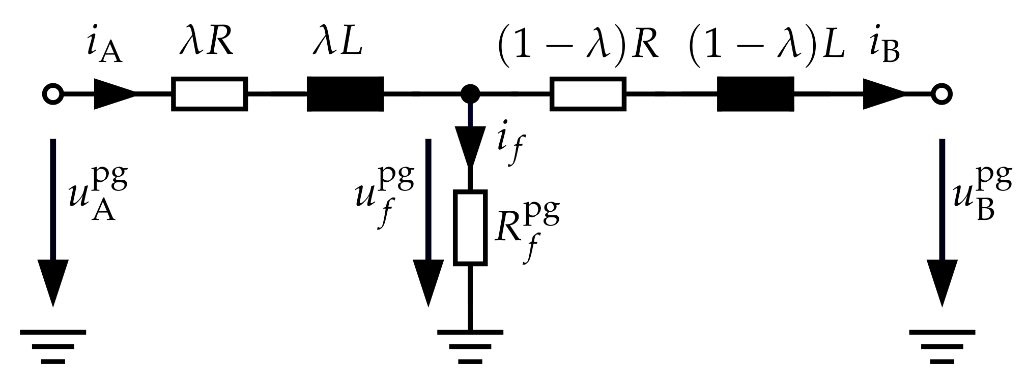
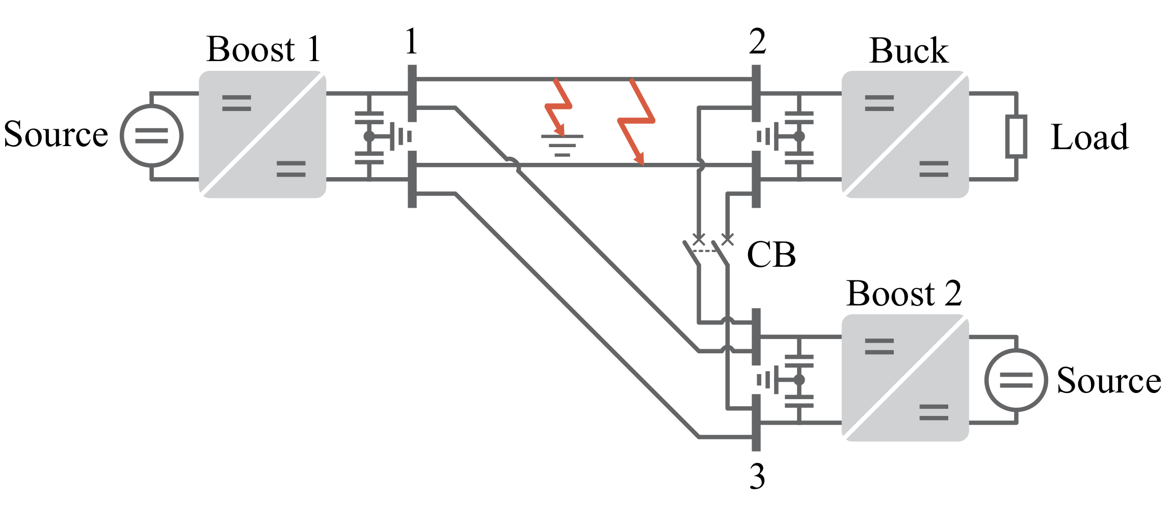
Beside the reviewed deficiencies of conventional online fault identification methods, most of the methods cover only the fault conditions with single-end current injection. Yet the protection of MTDC distribution grids, in which fault currents are contributed by multiple power sources, entails a fault identification method that is applicable to both single- and double-end fault current injection modes. To fill this gap, an online fault identification method is introduced in this work, which makes use of the available communication infrastructure and measurement sensors in MTDC distribution grids. First, a generic model of DC cables with pole-to-ground (PG) or pole-to-pole (PP) faults is developed. On this basis, a Kalman filter is established to reconstruct the fault distance and resistance with single- and double-end current injection. Through the real-time simulation of various PG and PP fault scenarios in a three-terminal DC distribution grid, the accuracy and speed of the proposed online fault identification method are verified. Compared with the existing online fault identification methods, the advantageous features of the proposed method include:

(1)

The proposed fault identification method can cover both PG and PP faults in DC lines with single- or double-ended fault current injection, which has improved applicability in the protection of MTDC distribution grids.

(2)

Unlike those fault location methods that only estimate the fault distance, the proposed fault identification method also provides the estimated value of the fault resistance, with which the fault severity can be determined.

(3)

Using the Kalman filter-based parameter estimation algorithm, the proposed method can achieve fast fault identification with a short response time of less than 1 ms. Its speed and effectiveness in different fault scenarios were verified through real-time simulation.

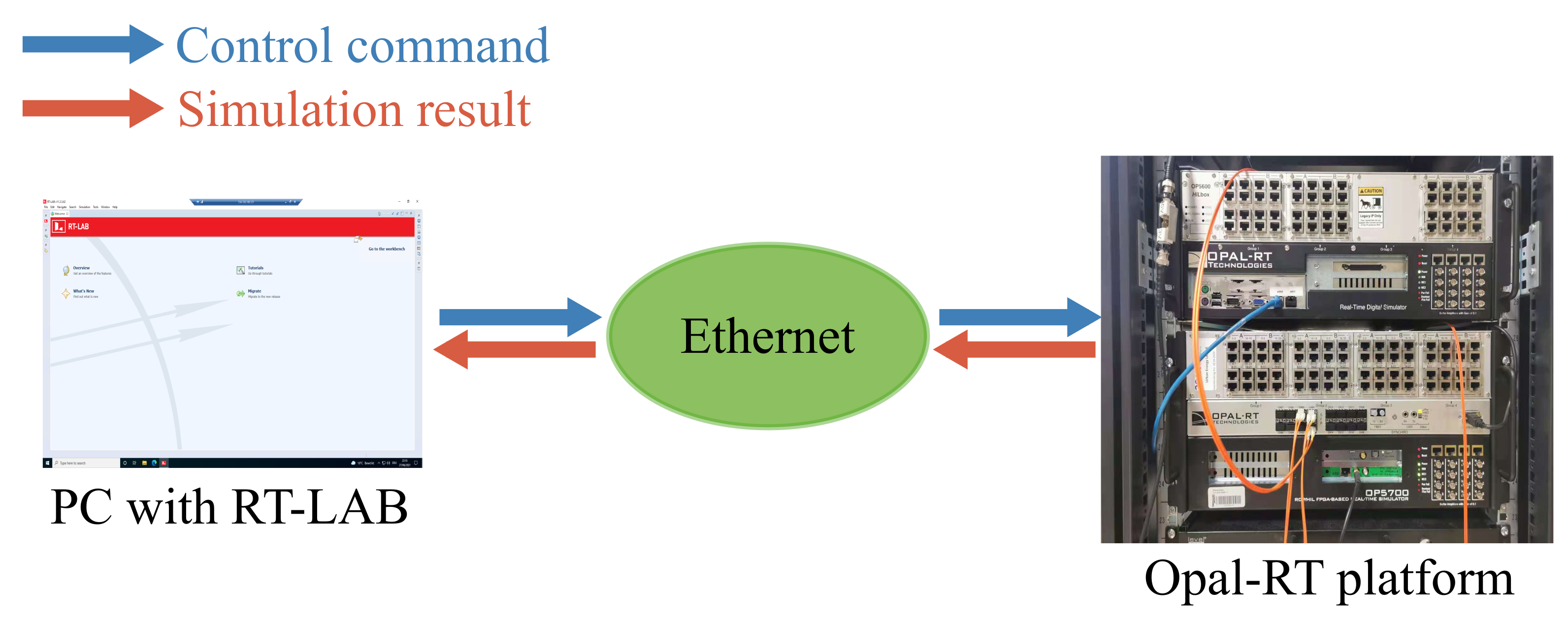
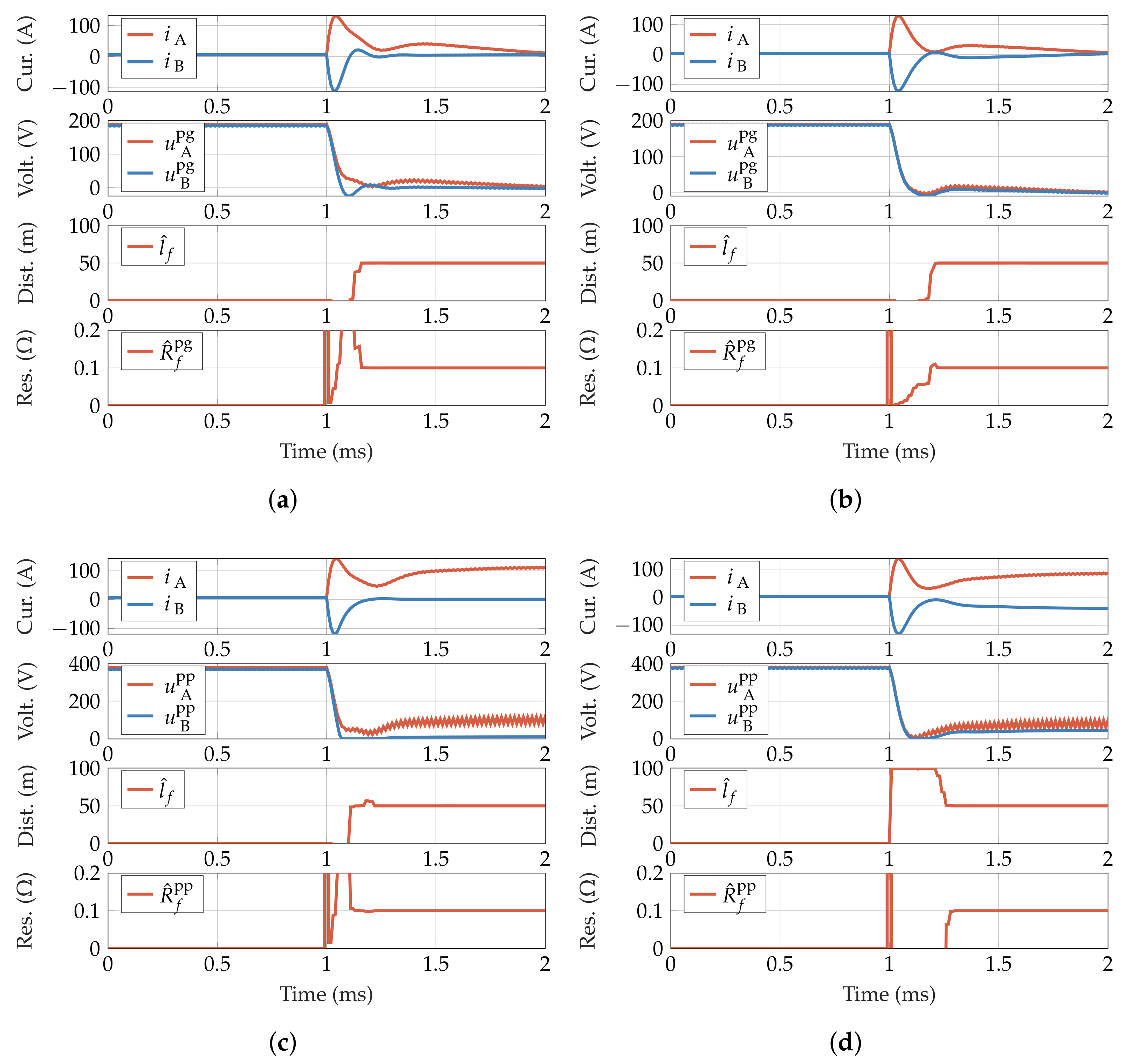
The remainder of this paper is structured in this way: Section 2 discusses the major challenges to online fault identification in MTDC distribution grids. Section 3 develops the mathematical models of the DC lines with PG and PP faults. Section 4 introduces the parameter estimation algorithm and presents the complete procedures of the proposed online fault identification approach. Section 5 verifies the performance of this fault identification method through real-time simulation. Section 6 concludes the paper.

2. Challenges to Online Fault Identification in MTDC Distribution Grids

In this section, the major challenges in the implementation of online fault identification functions in MTDC grids are first reviewed.

2.1. Grid Architecture

To improve the reliability of power supply, MTDC distribution grids are often of ring or meshed topologies [22]. A typical MTDC distribution grid is shown in Figure 2.

When a short-circuit fault occurs in such a system, the DC-link capacitors of multiple converters directly discharge towards the fault point. The sum of the capacitive discharge currents flowing to the fault is given by

$$\begin{array}{c}\hfill i_{\mathrm{fault},\mathrm{dis}}=\sum _{k=1}^n{i}_{\mathrm{dis},k}\end{array}$$

(1)

where n is the number of DC-link capacitors that discharge into the fault [23]. In this condition, the fault currents from multiple sources flow into both ends of the faulty line. Therefore, a fault identification method that is fit for the double-end fault current injection is needed for the protection of MTDC distribution grids.

2.2. Response Time

In order to prevent irreversible thermal damages to power electronic devices, the faulty lines in MTDC distribution grids must be disconnected as early as possible. As a result, little response time is available for fault identification in MTDC distribution grids, which can be expressed by [18]

$$\begin{array}{c}\hfill t_{\mathrm{FI}}\le t_{\max }-t_{\mathrm{CB}}-t_{\mathrm{com}}\end{array}$$

(2)

where $t_{\mathrm{FI}}$ is the response time of fault identification. $t_{\max }$ denotes the maximum tolerance time of power electronic devices to short-circuit currents, which is in the range of milliseconds [3]. $t_{\mathrm{CB}}$ is the operation time of circuit breakers, ranging from several microseconds to tens of milliseconds according to the circuit breaker design [24]. $t_{\mathrm{com}}$ is the communication latency. As can be seen in (2) the fault identification must be achieved within a few milliseconds after fault.

2.3. Grounding Strategy

According to system grounding strategies, monopolar DC systems can be categorized into asymmetrical and symmetrical types [25,26], in which the current loops of both PG and PP faults are illustrated in Figure 3.

In the asymmetrical monopolar DC system (Figure 3a), the negative pole of DC-link is grounded. In case of either PG or PP fault, the DC-link voltage drops to a low level while a permanent over-current flows through the faulty pole of the cable. In this sense, PG and PP faults exert the similar impacts to asymmetrical monopolar DC systems.

In the symmetrical monopolar DC system (Figure 3b), the midpoint of DC-link is grounded. In this case, PP faults lead to permanent over-currents and under-voltages in both poles. Yet, a PG fault discharges only the faulty pole. In this condition, the fault current is just a temporary discharge current.

From the view point of protection, the PG faults in symmetrical DC grids are the most challenging condition to fault identification because of the zero values of steady-state fault currents. Therefore, to cover the worst-case scenario, we will consider a symmetrical DC grid model as the study case in Section 5.

3. DC Line Model

As the theoretical foundation of the model-based fault identification method in MTDC distribution grids, a generic model of DC lines with PP and PG short-circuit faults is introduced in this section. On this basis, the equations for fault parameter estimation are derived.

3.1. DC Line Model with PG Fault

The model of a single DC line with a PG fault is illustrated in Figure 4, in which $u_{\mathrm{A}}^{\mathrm{pg}}$ and $u_{\mathrm{B}}^{\mathrm{pg}}$ are the PG voltages, $i_{\mathrm{A}}$ and $i_{\mathrm{B}}$ the line currents measured at both ends, $R_{}$ and $L_{}$ the line resistance and line inductance while the line capacitance is ignored, $R_f^{\mathrm{pg}}$ the PG fault resistance, $u_f^{\mathrm{pg}}$ the PG voltage at the fault location, $i_f$ the fault current and $\lambda$ the fault distance factor as the percentage of fault distance against cable length. There are the following mathematical relationships in this model:

$$\begin{array}{cc}\hfill u_f^{\mathrm{pg}}=& u_{\mathrm{A}}^{\mathrm{pg}}-\lambda R_{}{i}_{\mathrm{A}}-\lambda L_{}\frac{d{i}_{\mathrm{A}}}{dt}\hfill \\ \end{array}$$

(3)

$$\begin{array}{cc}\hfill u_f^{\mathrm{pg}}=& u_{\mathrm{B}}^{\mathrm{pg}}+(1-\lambda )R_{}{i}_{\mathrm{B}}+(1-\lambda )L_{}\frac{d{i}_{\mathrm{B}}}{dt}\hfill \\ \end{array}$$

(4)

$$\begin{array}{cc}\hfill u_f^{\mathrm{pg}}=& R_f^{\mathrm{pg}}(i_{\mathrm{A}}-i_{\mathrm{B}})\hfill \\ \end{array}$$

(5)

$$\begin{array}{cc}\hfill i_f=& i_{\mathrm{A}}-i_{\mathrm{B}}\hfill \end{array}$$

(6)

Based on (3), (4), (5) and (6), the derivative of $i_f$ can be expressed as:

$$\begin{array}{cc}\hfill \frac{d{i}_f}{dt}=& \frac{d{i}_{\mathrm{A}}}{dt}-\frac{d{i}_{\mathrm{B}}}{dt}\hfill \\ \hfill =& -\left(\frac{R_f^{\mathrm{pg}}}{\lambda L_{}}+\frac{R_f^{\mathrm{pg}}}{(1-\lambda )L_{}}+\frac{R_{}}{L_{}}\right)i_f+\frac{1}{\lambda L_{}}{u}_{\mathrm{A}}^{\mathrm{pg}}+\frac{1}{(1-\lambda )L_{}}{u}_{\mathrm{B}}^{\mathrm{pg}}\hfill \end{array}$$

(7)

3.2. DC Line Model with PP Fault

The DC line model with a PP fault is illustrated in Figure 5. In this case, $u_{\mathrm{A}}^{\mathrm{pp}}$ and $u_{\mathrm{B}}^{\mathrm{pp}}$ are the PP voltages at both ends, $R_f^{\mathrm{pp}}$ the PP fault resistance and $u_f^{\mathrm{pp}}$ the PP voltage at the fault location. In this model, the following relationships hold:

$$\begin{array}{cc}\hfill u_f^{\mathrm{pp}}=& u_{\mathrm{A}}^{\mathrm{pp}}-2\lambda R_{}{i}_{\mathrm{A}}-2\lambda L_{}\frac{d{i}_{\mathrm{A}}}{dt}\hfill \\ \end{array}$$

(8)

$$\begin{array}{cc}\hfill u_f^{\mathrm{pp}}=& u_{\mathrm{B}}^{\mathrm{pp}}+2(1-\lambda )R_{}{i}_{\mathrm{B}}+2(1-\lambda )L_{}\frac{d{i}_{\mathrm{B}}}{dt}\hfill \\ \end{array}$$

(9)

$$\begin{array}{cc}\hfill u_f^{\mathrm{pp}}=& R_f^{\mathrm{pp}}(i_{\mathrm{A}}-i_{\mathrm{B}})\hfill \\ \end{array}$$

(10)

$$\begin{array}{cc}\hfill i_f=& i_{\mathrm{A}}-i_{\mathrm{B}}\hfill \end{array}$$

(11)

Similarly, the expression of $d{i}_f/dt$ in PP faults can be derived from (8), (9), (10) and (11):

$$\begin{array}{c}\hfill \begin{array}{cc}\hfill \frac{d{i}_f}{dt}=& \frac{d{i}_{\mathrm{A}}}{dt}-\frac{d{i}_{\mathrm{B}}}{dt}\hfill \\ \hfill =& -\left(\frac{R_f^{\mathrm{pp}}}{2\lambda L_{}}+\frac{R_f^{\mathrm{pp}}}{2(1-\lambda )L_{}}+\frac{R_{}}{L_{}}\right)i_f+\frac{1}{2\lambda L_{}}{u}_{\mathrm{A}}^{\mathrm{pp}}+\frac{1}{2(1-\lambda )L_{}}{u}_{\mathrm{B}}^{\mathrm{pp}}\hfill \end{array}\end{array}$$

(12)

3.3. Representation of Fault Parameters

Comparing (7) and (12), we can derive a unified representation of $d{i}_f/dt$ in both PG and PP faults:

$$\begin{array}{c}\hfill \begin{array}{cc}\hfill \frac{d{i}_f}{dt}=& -\left(\frac{R_f}{\lambda L_{}}+\frac{R_f}{(1-\lambda )L_{}}+\frac{R_{}}{L_{}}\right)i_f+\frac{1}{\lambda L_{}}{u}_{\mathrm{A}}+\frac{1}{(1-\lambda )L_{}}{u}_{\mathrm{B}}\hfill \end{array}\end{array}$$

(13)

where

$$\{R_f,u_{\mathrm{A}},u_{\mathrm{B}}\}=\left\{\begin{array}{c}\{R_f^{\mathrm{pg}},u_{\mathrm{A}}^{\mathrm{pg}},u_{\mathrm{B}}^{\mathrm{pg}}\}\mathrm{in}\mathrm{PG}\mathrm{faults},\hfill \\ \{R_f^{\mathrm{pp}}/2,u_{\mathrm{A}}^{\mathrm{pp}}/2,u_{\mathrm{B}}^{\mathrm{pp}}/2\}\mathrm{in}\mathrm{PP}\mathrm{faults}\hfill \end{array}\right.$$

Performing Laplace transform to (13) yields:

$$I_f\left(s\right)={\displaystyle \frac{(1-\lambda )U_{\mathrm{A}}\left(s\right)+\lambda U_{\mathrm{B}}\left(s\right)}{(1-\lambda )\lambda L_{}s+R_f+(1-\lambda )\lambda R_{}}}$$

(14)

Transforming (14) into discrete-time domain with backward Euler method yields:

$$\begin{array}{cc}\hfill i_f\left(k\right)=& {\displaystyle \frac{(1-\lambda )\lambda L_{}}{D}}{i}_f(k-1)+{\displaystyle \frac{(1-\lambda )T_{\mathrm{s}}}{D}}{u}_{\mathrm{A}}\left(k\right)+{\displaystyle \frac{\lambda T_{\mathrm{s}}}{D}}{u}_{\mathrm{B}}\left(k\right)\hfill \end{array}$$

(15)

where $D=(1-\lambda )\lambda L_{}+(1-\lambda )\lambda R_{}{T}_{\mathrm{s}}+R_f{T}_{\mathrm{s}}$ and $T_{\mathrm{s}}$ is the sampling step.

Rewriting (15) in matrix form yields:

$$\left[\begin{array}{c}{i}_f\left(k\right)\end{array}\right]=\left[\begin{array}{ccc}{i}_f(k-1)& u_{\mathrm{A}}\left(k\right)& u_{\mathrm{B}}\left(k\right)\end{array}\right]\left[\begin{array}{c}{\theta }_1\left(k\right)\\ {\theta }_2\left(k\right)\\ {\theta }_3\left(k\right)\end{array}\right]$$

(16)

where

$$\begin{array}{cc}\hfill {\theta }_1& ={\displaystyle \frac{(1-\lambda )\lambda L_{}}{(1-\lambda )\lambda L_{}+(1-\lambda )\lambda R_{}{T}_{\mathrm{s}}+R_f{T}_{\mathrm{s}}}}\hfill \end{array}$$

(17)

$$\begin{array}{cc}\hfill {\theta }_2& ={\displaystyle \frac{(1-\lambda )T_{\mathrm{s}}}{(1-\lambda )\lambda L_{}+(1-\lambda )\lambda R_{}{T}_{\mathrm{s}}+R_f{T}_{\mathrm{s}}}}\hfill \end{array}$$

(18)

$$\begin{array}{cc}\hfill {\theta }_3& ={\displaystyle \frac{\lambda T_{\mathrm{s}}}{(1-\lambda )\lambda L_{}+(1-\lambda )\lambda R_{}{T}_{\mathrm{s}}+R_f{T}_{\mathrm{s}}}}\hfill \end{array}$$

(19)

From (17), (18) and (19), following expressions are obtained:

$$\lambda =\frac{T_{\mathrm{s}}{\theta }_1}{L_{}{\theta }_2}=1-\frac{T_{\mathrm{s}}{\theta }_1}{L_{}{\theta }_3}$$

(20)

$$\begin{array}{cc}\hfill R_f& =\frac{L^2{\theta }_2-L^2{\theta }_1{\theta }_2+T_{\mathrm{s}}^{2}R{\theta }_1^2-T_{\mathrm{s}}L{\theta }_1+T_{\mathrm{s}}L{\theta }_1^2-T_{\mathrm{s}}LR{\theta }_1{\theta }_2}{L^2{\theta }_2^2}\hfill \\ \hfill & =\frac{L^2{\theta }_3-L^2{\theta }_1{\theta }_3+T_{\mathrm{s}}^{2}R{\theta }_1^2-T_{\mathrm{s}}L{\theta }_1+T_{\mathrm{s}}L{\theta }_1^2-T_{\mathrm{s}}LR{\theta }_1{\theta }_3}{L^2{\theta }_3^2}\hfill \end{array}$$

(21)

From (20) and (21), we can see that $\lambda$ and $R_f$ are depending on ${\theta }_1$, ${\theta }_2$ and ${\theta }_3$. Therefore, the task of fault identification becomes the estimation of ${\theta }_1$, ${\theta }_2$ and ${\theta }_3$.

4. Fault Identification Method

In Section 3, the model of faulty lines in MTDC distribution grids has been established, yet a mathematical tool to extract the fault information is still needed. In this section, a Kalman filter-based fault parameter estimation method is introduced. Afterwards, the procedures of the proposed fault identification method are presented.

4.1. Kalman Filter Algorithm

Kalman filter is a widely used mathematical tool to estimate unknown states and parameters, which is advantageous in terms of convergence speed and estimation accuracy [27,28]. The parameter estimation problem can be represented as

$$\begin{array}{cc}\hfill y\left(k\right)=& \varphi \left(k\right)\theta \left(k\right)+v\left(k\right)\hfill \end{array}$$

(22)

$$\begin{array}{cc}\hfill \theta \left(k\right)=& \theta (k-1)+w\left(k\right)\hfill \end{array}$$

(23)

where $y\left(k\right)\in {\mathbb{R}}^{m\times 1}$ is the matrix of measurement outputs, $\theta \left(k\right)\in {\mathbb{R}}^{n\times 1}$ the matrix of parameters to estimate, $\varphi \left(k\right)\in {\mathbb{R}}^{m\times n}$ the regression matrix, $v\left(k\right)\in {\mathbb{R}}^{m\times 1}$ and $w\left(k\right)\in {\mathbb{R}}^{n\times 1}$ the measurement and process noises, respectively. For uncorrelated noises v and w, their covariance matrices are denoted by $R\in {\mathbb{R}}^{m\times m}$ and $Q\in {\mathbb{R}}^{n\times n}$, respectively.

The parameter estimation is achieved through recursive prediction and correction:

Prediction:

$$\begin{array}{cc}\hfill {\widehat{\theta }}^{-}\left(k\right)=& \widehat{\theta }(k-1)\hfill \end{array}$$

(24)

$$\begin{array}{cc}\hfill P^{-}\left(k\right)=& P(k-1)+Q\hfill \\ \end{array}$$

(25)

where $\widehat{\theta }\left(k\right)$ is the estimate of parameter matrix, $P\left(k\right)$ is the covariance matrix of estimation error. The "−" superscript denotes that the predicted value is prior.

Correction:

$$\begin{array}{cc}\hfill \widehat{\theta }\left(k\right)=& {\widehat{\theta }}^{-}\left(k\right)+K\left(k\right)\left(y\left(k\right)-\varphi \left(k\right){\widehat{\theta }}^{-}\left(k\right)\right)\hfill \\ \end{array}$$

(26)

$$\begin{array}{cc}\hfill P\left(k\right)=& \left(I-K\left(k\right)\varphi \left(k\right)\right)P^{-}\left(k\right)\hfill \end{array}$$

(27)

where

$$\begin{array}{c}\hfill K\left(k\right)=P^{-}\left(k\right){\varphi }^T\left(k\right){\left(\varphi \left(k\right)P^{-}\left(k\right){\varphi }^T\left(k\right)+R\right)}^{-1}\end{array}$$

(28)

Through the iteration of prediction and correction, $\widehat{\theta }\left(k\right)$ converges, which is taken as the estimate of $\theta$.

Comparing (22) and (16), we can define y, $\varphi$ and $\theta$ in our case:

$$\begin{array}{cc}\hfill y\left(k\right)=& \left[i_f\left(k\right)\right]\hfill \end{array}$$

(29)

$$\begin{array}{cc}\hfill \varphi \left(k\right)=& \left[\begin{array}{ccc}{i}_f(k-1)& u_{\mathrm{A}}\left(k\right)& u_{\mathrm{B}}\left(k\right)\end{array}\right]\hfill \\ \end{array}$$

(30)

$$\begin{array}{cc}\hfill \theta \left(k\right)=& {\left[\begin{array}{ccc}{\theta }_1\left(k\right)& {\theta }_2\left(k\right)& {\theta }_3\left(k\right)\end{array}\right]}^T\hfill \\ \end{array}$$

(31)

Substituting (29) to (31) in (22) and (23) yields the Kalman filter equations.

4.2. Fault Identification Procedure

The procedures of the proposed fault identification algorithm are illustrated in Figure 6. As we can see, the complete process can be divided into three major steps, which are explained in the following.

(1)

Signal acquisition: the input values $i_f$, $u_{\mathrm{A}}$ and $u_{\mathrm{B}}$ are acquired in real time. To obtain $u_{\mathrm{A}}$ and $u_{\mathrm{B}}$ in PP and PG faults, either PP or PG node voltages are needed. Meanwhile, the fault current $i_f$ is calculated from the differential of the current signals measured at the both ends of faulty cable.

(2)

Kalman filter: with the known $i_f$, $u_{\mathrm{A}}$ and $u_{\mathrm{B}}$, y and $\varphi$ of the Kalman filter are obtained with (29) and (30) in real time. Then the iterative prediction and correction of Kalman filter algorithm are performed. The iteration converges when the relative error between two sequential $\widehat{\theta }$ is below a threshold ${\theta }_{\mathrm{th}}$, i.e.

$$\begin{array}{c}\hfill \Delta \widehat{\theta }\left(k\right)=\max \left\{\left|\frac{{\widehat{\theta }}_i\left(k\right)-{\widehat{\theta }}_i(k-1)}{{\widehat{\theta }}_i\left(k\right)}\right|\right\}<{\theta }_{\mathrm{th}},i=1,2,3.\end{array}$$

(32)

When (32) is met, $\widehat{\theta }\left(k\right)$ is taken as the best estimate of $\theta$.

(3)

Fault parameter calculation: based on $\widehat{\theta }\left(k\right)$, the estimates of fault distance factor $\widehat{\lambda }$ and the fault resistance ${\widehat{R}}_f$ can be obtained with (20) and (21), respectively. With $\widehat{\lambda }$, the fault distance ${\widehat{l}}_f$ can be obtained:

$$\begin{array}{c}\hfill {\widehat{l}}_f=\widehat{\lambda }l\end{array}$$

(33)

where l is the length of the cable. At last, according the fault type, the fault resistance ${\widehat{R}}_f^{\mathrm{pg}}$ or ${\widehat{R}}_f^{\mathrm{pp}}$ is determined based on ${\widehat{R}}_f$.

5. Verification Test

In this section, the proposed fault identification method is verified through the real-time simulation of different fault scenarios in a three-terminal DC distribution grid. Then the performance of this method is compared with those of existing methods.

5.1. System Model

In order to verify the performance of the proposed fault identification method in MTDC distribution grids, different fault scenarios in a three-terminal DC system were simulated with Opal-RT real-time simulator. The system diagram is shown in Figure 7. Furthermore, the component parameters are listed in

Table 1. Parameters of the MTDC Distribution Grid Model.

Component	Parameter	Value
boost converter	rated voltage (input/output)	190 V DC/380 V DC
	rated power	5 kW
	switching frequency	50 kHz
buck converter	rated voltage (input/output)	380 V DC/190 V DC
	rated power	5 kW
	switching frequency	50 kHz
DC cable	resistance per unit length	8 $\mathrm{\Omega }$/km
	inductance per unit length	$0.45$ mH/km
	capacitance per unit length	$0.1$$\mathsf{\mu }$F/km
	length	$0.1$ km

. As we can see in Figure 7 that there are two boost converters in the system, which are interfaced with two independent power sources. The buck converter feeds a resistive load. The three converters are interconnected by DC cables. The midpoints of DC links are grounded, making this grid a symmetrical monopolar DC system. We simulated both PG and PP faults in Line 12 connecting Node 1 and Node 2. To simulate both single-end and double-end fault current injection modes, an interconnection DC circuit breaker CB is installed in Line 23. When CB is open, the fault current in Line 12 is injected from Node 1. When CB is closed, the fault current is fed from both Node 1 and Node 2.

5.2. Test Setup

The test bench of the proposed fault identification algorithm is illustrated in Figure 8. The simulation of the three-terminal DC distribution grid and the implementation of the fault identification algorithm are achieved with the real-time simulator OP5700 in the Opal-RT platform. The control of the Opal-RT target and the data-recording during the real-time test are through the RT-LAB software in a separate computer, which communicates with the Opal-RT target through Ethernet. With this test setup, the performance of the proposed fault identification method can be verified in an online environment. The simulated fault scenarios are listed in

Table 2. Simulation Parameters.

Parameter	Value
sampling step $T_{\mathrm{s}}$	10 $\mathsf{\mu }$s
fault type	PG and PP
fault current injection	single-end and double-end
fault location factor $\lambda$	$10\%$, $30\%$, $50\%$, $70\%$, $90\%$
fault resistance $R_f$	$0.01$$\mathrm{\Omega }$, $0.1$$\mathrm{\Omega }$, 1 $\mathrm{\Omega }$, 10 $\mathrm{\Omega }$
convergence threshold ${\theta }_{\mathrm{th}}$	$5\ast {10}^{-4}$

.

5.3. Influences of Fault Types and Current Injection Modes

First, we tested the proposed fault identification method in PG and PP faults with both single-end and double-end fault current injections. The fault location is the midpoint of Line 12, i.e., $l_f=50$ m, and the fault resistance $R_f=0.1\mathrm{\Omega }$ (for both PG and PP faults). The test results are plotted in Figure 9. Based on these results, the responses of the proposed fault identification method to PG and PP fault types in the two current injection modes are discussed in the following.

5.3.1. Fault Types

In PG faults (Figure 9a,b), the transient over-currents $i_{\mathrm{A}}$ and $i_{\mathrm{B}}$ decay to zero within 1 ms after the fault occurrence. In the meantime, the PG voltages $u_{\mathrm{A}}^{\mathrm{pg}}$ and $u_{\mathrm{B}}^{\mathrm{pg}}$ also drop to zero, indicating that the DC-link capacitors of the faulty pole are fully discharged. These results validate the conclusion about PG faults in Section 2.3: there are only transient current impacts caused by PG faults on symmetrical monopolar DC systems. In the PP faults (Figure 9c,d) we can see the permanent over-currents ($i_{\mathrm{A}}$ in Figure 9c, $i_{\mathrm{A}}$ and $i_{\mathrm{B}}$ in Figure 9d) after the fault occurrence. Meanwhile, node voltages drop to low values in the steady state of fault. These results verify that the PP faults exert permanent influences on the system, as discussed in Section 2.3.

Besides, we can see that in PG faults, the resulted over-currents last for about 1 ms before decaying to zero. Therefore, online fault identification functions must be able to respond within such a short time otherwise the fault current might become too tiny to measure. This requirement can be satisfied with the proposed fault identification method. As can be seen in Figure 9 that ${\widehat{R}}_f^{\mathrm{pg}}$, ${\widehat{R}}_f^{\mathrm{pp}}$ and ${\widehat{l}}_f$ converge at their true values within less than $0.5$ ms, which validates the fastness of the proposed method.

5.3.2. Fault Current Injection Mode

The influence of the fault current injection mode is discussed based on the test results of PP faults in Figure 9c,d. In both Figure 9c,d, when the PP fault occurs at $t=1$ ms, $i_{\mathrm{A}}$ and $i_{\mathrm{B}}$ undergo surges in opposite directions. As time goes, we can see the effects of different fault current injection modes. In the case of single-end fault current injection (Figure 9c), $i_{\mathrm{B}}$ drops to zero in the steady state. This is because Line 23 is disconnected by CB in this case, so no fault current is fed by Node 2 into Line 12. In case of double-end fault current injection (Figure 9d), both $i_{\mathrm{A}}$ and $i_{\mathrm{B}}$ are non-zero values in the steady state. This is because when CB is closed, the fault current in Line 12 is fed from both Node 1 and Node 2.

Because of the existence of multiple power sources in MTDC distribution grids, the possibilities of both single- and double-end fault current injections have to be taken into consideration in fault identification. This demand can be met with the proposed fault identification method as it responds accurately and timely in both fault conditions.

5.4. Accuracy and Response Time

To quantify the response speed of the proposed fault identification method, the response time $\tau$ was measured, which is the duration from the fault occurrence until the fault parameters are obtained. To evaluate the accuracy of fault identification, the estimation errors in fault distance ${\delta }_{\lambda }$ and fault resistance ${\delta }_R$ were calculated:

$$\begin{array}{cc}\hfill {\delta }_{\lambda }& =|\lambda -\widehat{\lambda }|\hfill \end{array}$$

(34)

$$\begin{array}{cc}\hfill {\delta }_R& =\left|\frac{R_f-{\widehat{R}}_f}{R_f}\right|\times 100\%\hfill \end{array}$$

(35)

$\tau$, ${\delta }_{\lambda }$ and ${\delta }_R$ in the various fault scenarios defined in Table 2 are summarized in

Table 3. Test Results of PG Faults with Single-End Fault Current Injection.

	${\mathit{R}}_{\mathit{f}}$
	$\mathbf{0.01}$$\mathbf{\Omega }$			$\mathbf{0.1}$$\mathbf{\Omega }$			1 $\mathbf{\Omega }$			10 $\mathbf{\Omega }$
$\mathbf{\lambda }(\%)$	$\mathbf{\tau }$ (ms)	${\mathbf{\delta }}_{\mathbf{\lambda }}(\%)$	${\mathbf{\delta }}_{\mathit{R}}(\%)$	$\mathbf{\tau }$ (ms)	${\mathbf{\delta }}_{\mathbf{\lambda }}(\%)$	${\mathbf{\delta }}_{\mathit{R}}(\%)$	$\mathbf{\tau }$ (ms)	${\mathbf{\delta }}_{\mathbf{\lambda }}(\%)$	${\mathbf{\delta }}_{\mathit{R}}(\%)$	$\mathbf{\tau }$ (ms)	${\mathbf{\delta }}_{\mathbf{\lambda }}(\%)$	${\mathbf{\delta }}_{\mathit{R}}(\%)$
10	$0.15$	$0.00$	$0.01$	$0.16$	$0.00$	$0.00$	$0.20$	$0.01$	$0.03$	$0.50$	$1.50$	$1.73$
30	$0.17$	$0.00$	$0.28$	$0.19$	$0.00$	$0.01$	$0.21$	$0.01$	$0.04$	$0.44$	$2.62$	$3.84$
50	$0.20$	$0.01$	$0.15$	$0.19$	$0.01$	$0.04$	$0.22$	$\mathbf{0}.\mathbf{10}$	$0.23$	$0.34$	$\mathbf{4.95}$	$\mathbf{10.11}$
70	$0.17$	$0.00$	$0.02$	$0.18$	$0.00$	$0.03$	$0.18$	$0.03$	$0.06$	$0.50$	$2.56$	$3.88$
90	$0.20$	$0.00$	$0.03$	$0.28$	$0.02$	$0.01$	$0.24$	$0.01$	$0.06$	$\mathbf{1.07}$	$1.37$	$1.74$

,

Table 4. Test Results of PP Faults with Single-End Fault Current Injection.

	${\mathit{R}}_{\mathit{f}}$
	$\mathbf{0.01}$$\mathbf{\Omega }$			$\mathbf{0.1}$$\mathbf{\Omega }$			1 $\mathbf{\Omega }$			10 $\mathbf{\Omega }$
$\mathbf{\lambda }(\%)$	$\mathbf{\tau }$ (ms)	${\mathbf{\delta }}_{\mathbf{\lambda }}(\%)$	${\mathbf{\delta }}_{\mathit{R}}(\%)$	$\mathbf{\tau }$ (ms)	${\mathbf{\delta }}_{\mathbf{\lambda }}(\%)$	${\mathbf{\delta }}_{\mathit{R}}(\%)$	$\mathbf{\tau }$ (ms)	${\mathbf{\delta }}_{\mathbf{\lambda }}(\%)$	${\mathbf{\delta }}_{\mathit{R}}(\%)$	$\mathbf{\tau }$ (ms)	${\mathbf{\delta }}_{\mathbf{\lambda }}(\%)$	${\mathbf{\delta }}_{\mathit{R}}(\%)$
10	$\mathbf{0.38}$	$0.00$	$0.01$	$0.28$	$0.00$	$0.00$	$0.27$	$0.00$	$0.01$	$0.38$	$0.49$	$0.59$
30	$0.36$	$0.00$	$0.12$	$0.27$	$0.00$	$0.01$	$0.21$	$0.00$	$0.01$	$0.38$	$0.70$	$0.59$
50	$0.36$	$0.00$	$0.33$	$0.26$	$0.00$	$0.01$	$0.22$	$0.02$	$0.05$	$0.20$	$1.19$	$2.46$
70	$0.35$	$0.01$	$0.31$	$0.22$	$0.00$	$0.00$	$0.20$	$0.01$	$0.02$	$0.41$	$0.60$	$0.97$
90	$0.30$	$0.00$	$0.03$	$0.15$	$0.00$	$0.10$	$0.22$	$0.01$	$0.04$	$0.52$	$0.32$	$0.49$

,

Table 5. Test Results of PG Faults with Double-End Fault Current Injection.

	${\mathit{R}}_{\mathit{f}}$
	$\mathbf{0.01}$$\mathbf{\Omega }$			$\mathbf{0.1}$$\mathbf{\Omega }$			1 $\mathbf{\Omega }$			10 $\mathbf{\Omega }$
$\mathbf{\lambda }(\%)$	$\mathbf{\tau }$ (ms)	${\mathbf{\delta }}_{\mathbf{\lambda }}(\%)$	${\mathbf{\delta }}_{\mathit{R}}(\%)$	$\mathbf{\tau }$ (ms)	${\mathbf{\delta }}_{\mathbf{\lambda }}(\%)$	${\mathbf{\delta }}_{\mathit{R}}(\%)$	$\mathbf{\tau }$ (ms)	${\mathbf{\delta }}_{\mathbf{\lambda }}(\%)$	${\mathbf{\delta }}_{\mathit{R}}(\%)$	$\mathbf{\tau }$ (ms)	${\mathbf{\delta }}_{\mathbf{\lambda }}(\%)$	${\mathbf{\delta }}_{\mathit{R}}(\%)$
10	$0.15$	$0.00$	$0.01$	$0.13$	$0.00$	$0.00$	$0.20$	$0.00$	$0.04$	$0.52$	$1.98$	$2.35$
30	$0.20$	$0.00$	$0.13$	$0.20$	$0.00$	$0.03$	$0.22$	$0.02$	$0.07$	$0.36$	$3.06$	$4.53$
50	$0.25$	$0.00$	$0.07$	$0.24$	$0.01$	$0.03$	$0.28$	$0.06$	$0.01$	$0.22$	$4.52$	$9.12$
70	$0.23$	$0.01$	$0.17$	$0.20$	$0.01$	$0.01$	$0.15$	$0.01$	$0.03$	$0.42$	$2.65$	$4.03$
90	$0.20$	$0.00$	$0.12$	$0.20$	$0.01$	$0.01$	$0.18$	$0.00$	$0.02$	$0.52$	$1.72$	$2.09$

,

Table 6. Test Results of PP Faults with Double-End Fault Current Injection.

	${\mathit{R}}_{\mathit{f}}$
	$\mathbf{0.01}$$\mathbf{\Omega }$			$\mathbf{0.1}$$\mathbf{\Omega }$			1 $\mathbf{\Omega }$			10 $\mathbf{\Omega }$
$\mathbf{\lambda }(\%)$	$\mathbf{\tau }$ (ms)	${\mathbf{\delta }}_{\mathbf{\lambda }}(\%)$	${\mathbf{\delta }}_{\mathit{R}}(\%)$	$\mathbf{\tau }$ (ms)	${\mathbf{\delta }}_{\mathbf{\lambda }}(\%)$	${\mathbf{\delta }}_{\mathit{R}}(\%)$	$\mathbf{\tau }$ (ms)	${\mathbf{\delta }}_{\mathbf{\lambda }}(\%)$	${\mathbf{\delta }}_{\mathit{R}}(\%)$	$\mathbf{\tau }$ (ms)	${\mathbf{\delta }}_{\mathbf{\lambda }}(\%)$	${\mathbf{\delta }}_{\mathit{R}}(\%)$
10	$0.24$	$0.00$	$0.01$	$0.23$	$0.00$	$0.03$	$0.24$	$0.01$	$0.00$	$0.34$	$0.57$	$0.71$
30	$0.24$	$0.00$	$0.15$	$0.21$	$0.01$	$0.05$	$0.23$	$0.01$	$0.02$	$0.36$	$0.69$	$0.97$
50	$0.29$	$0.00$	$\mathbf{0.41}$	$0.31$	$0.01$	$0.01$	$0.30$	$0.02$	$0.01$	$0.34$	$1.25$	$2.54$
70	$0.22$	$0.01$	$0.03$	$0.21$	$0.00$	$0.02$	$0.16$	$0.01$	$0.01$	$0.28$	$0.70$	$1.11$
90	$0.20$	$0.00$	$0.09$	$0.24$	$0.00$	$0.03$	$0.16$	$0.00$	$0.01$	$0.36$	$0.51$	$0.66$

.

We can see that with the fault resistance up to 1 $\mathrm{\Omega }$, the proposed fault identification method has great performance. In this range, the fault location ${\widehat{l}}_f$ and resistance ${\widehat{R}}_f$ can be estimated with the maximum errors of $0.10\%$ and $0.41\%$, respectively. Furthermore, the maximum value of $\tau$ is $0.38$ ms. In the high-resistance (10 $\mathrm{\Omega }$) faults, the maximum value of $\tau$ reaches $1.07$ ms, and the maximum ${\delta }_{\lambda }$ and ${\delta }_R$ are $4.95\%$ and $10.11\%$, respectively.

5.5. Comparison with Existing Methods

The performance of the proposed fault identification method is also compared with those of the existing methods [8,10,17,18,21]. Since most of these works focus on low-resistance faults, a comparison with fault resistance up to $1\mathrm{\Omega }$ is shown in

Table 7. Comparison of Fault Identification Methods.

Method	Percentage Error		Response Time	Current Injection Mode	Additiona Requirement
	Distance	Resistance
[8]	$18.78\%$	N.A.	$0.65$ ms	single-end	No
[10]	$0.46\%$	N.A.	1 ms	N.A.	fault location module
[17]	$1.70\%$	N.A.	110 ms	double-end	communication
[18]	$2\%$	$2\%$	$4.1$ ms	double-end	No
[21]	$0.25\%$	$13.5\%$	$9.92$ ms	single-end	voltage divider
proposed	$0.10\%$	$0.41\%$	$0.38$ ms	single-/double-end	communication

. In this table, the impedance estimation-based fault location method [8] has an excessive fault location error $18.78\%$. The fault location module [10] has a low location error of $0.46\%$ and fast response time of 1 ms. The differential current-based fault location method in [17] achieves the fault location with a long response time of 110 ms. The iterative fault identification method [18] has the estimation errors in fault location and resistance of $2\%$, and the response time up to $4.1$ ms. Ref. [21] estimates fault location and resistance with a long response time of $9.92$ ms. At last, the proposed fault identification method has ${\delta }_{\lambda }=0.10\%$, ${\delta }_R=0.41\%$ and $\tau =0.38$ ms. Compared with the existing methods, the proposed method has significantly higher accuracy and faster response speed.

Besides that, we can also see that among all the existing methods, only [18,21] provide the information of both fault location and resistance, whereas the others estimate only the fault distance. As for the current injection mode, ref. [8,21] assume that the fault current is fed by only one end of the faulty line, whereas [17,18] consider the double-end current injection. The discussion of fault current inject mode is not applicable to [10] because it works when faulty lines are disconnected. All these functional limitations are overcome with the proposed fault identification method, which can estimate fault location and resistance in both single- and double-end current injection modes.

The specific requirements to implement these methods are also listed. Among all the six methods, ref. [8,18] require only local measurement signals. Ref. [17] and the proposed method are communication-based approaches. Ref. [10] is based on a fault location module. Ref. [21] needs the voltage signals measured from a voltage divider.

6. Conclusions

This paper introduces an online fault identification method for MTDC distribution grids, which is based on the parameter estimation in monitored DC lines. The proposed fault identification method has two advantageous features: (1) It is applicable to the faulty line with single- or double-end fault current injection. This feature makes the proposed fault identification method particularly suitable in the protection of MTDC distribution grids, which contain multiple distributed power sources. (2) It estimates not only the fault distance but also the fault resistance. Therefore, the fault severity can also be known. The test results in the real-time simulation show that the proposed online fault identification method can accurately identify different PG and PP faults with a short response time of less than 1 ms, which meets the requirement of speed in the fault identification in MTDC distribution grids. These results verify the effectiveness of this method as an online fault identification approach in MTDC distribution grids.

References

1. Siddique, H.A.B.; De Doncker, R.W. Evaluation of DC Collector-Grid Configurations for Large Photovoltaic Parks. IEEE Trans. Power Deliv. 2018, 33, 311–320. [Google Scholar] [CrossRef]
2. Xiao, L.; Lin, L.; Liu, Y. Discussions on the Architecture and Operation Mode of Future Power Grids. Energies 2011, 4, 1025–1035. [Google Scholar] [CrossRef] [Green Version]
3. Wang, T.; Monti, A.; Hu, J.; De Doncker, R.W. Protection of Dual-Active-Bridge Converters Against Underdamped Surge Current by Current Limiting Reactor. In Proceedings of the 2018 9th IEEE International Symposium on Power Electronics for Distributed Generation Systems (PEDG), Charlotte, NC, USA, 25–28 June 2018; pp. 1–6. [Google Scholar] [CrossRef]
4. Gertler, J.J. Survey of model-based failure detection and isolation in complex plants. IEEE Control Syst. Mag. 1988, 8, 3–11. [Google Scholar] [CrossRef]
5. Zhang, C.; Song, G.; Wang, T.; Yang, L. Single-Ended Traveling Wave Fault Location Method in DC Transmission Line Based on Wave Front Information. IEEE Trans. Power Deliv. 2019, 34, 2028–2038. [Google Scholar] [CrossRef]
6. Azizi, S.; Sanaye-Pasand, M.; Abedini, M.; Hasani, A. A Traveling-Wave-Based Methodology for Wide-Area Fault Location in Multiterminal DC Systems. IEEE Trans. Power Deliv. 2014, 29, 2552–2560. [Google Scholar] [CrossRef]
7. Nanayakkara, O.M.K.K.; Rajapakse, A.D.; Wachal, R. Traveling-Wave-Based Line Fault Location in Star-Connected Multiterminal HVDC Systems. IEEE Trans. Power Deliv. 2012, 27, 2286–2294. [Google Scholar] [CrossRef]
8. Feng, X.; Qi, L.; Pan, J. A Novel Fault Location Method and Algorithm for DC Distribution Protection. IEEE Trans. Ind. Appl. 2017, 53, 1834–1840. [Google Scholar] [CrossRef]
9. Christopher, E.; Sumner, M.; Thomas, D.W.P.; Wang, X.; de Wildt, F. Fault Location in a Zonal DC Marine Power System Using Active Impedance Estimation. IEEE Trans. Ind. Appl. 2013, 49, 860–865. [Google Scholar] [CrossRef]
10. Yang, Y.; Huang, C.; Xu, Q. A Fault Location Method Suitable for Low-Voltage DC Line. IEEE Trans. Power Deliv. 2020, 35, 194–204. [Google Scholar] [CrossRef]
11. Liu, W.; Liu, F.; Zha, X.; Huang, M.; Chen, C.; Zhuang, Y. An Improved SSCB Combining Fault Interruption and Fault Location Functions for DC Line Short-Circuit Fault Protection. IEEE Trans. Power Deliv. 2019, 34, 858–868. [Google Scholar] [CrossRef]
12. Yang, Q.; Li, J.; Le Blond, S.; Wang, C. Artificial neural network based fault detection and fault location in the DC microgrid. Energy Procedia 2016, 103, 129–134. [Google Scholar] [CrossRef]
13. Karmacharya, I.M.; Gokaraju, R. Fault Location in Ungrounded Photovoltaic System Using Wavelets and ANN. IEEE Trans. Power Deliv. 2018, 33, 549–559. [Google Scholar] [CrossRef]
14. Johnson, J.M.; Yadav, A. Complete protection scheme for fault detection, classification and location estimation in HVDC transmission lines using support vector machines. IET Sci. Meas. Technol. 2017, 11, 279–287. [Google Scholar] [CrossRef]
15. Tzelepis, D.; Dyśko, A.; Fusiek, G.; Niewczas, P.; Mirsaeidi, S.; Booth, C.; Dong, X. Advanced fault location in MTDC networks utilising optically-multiplexed current measurements and machine learning approach. Int. J. Electr. Power Energy Syst. 2018, 97, 319–333. [Google Scholar] [CrossRef] [Green Version]
16. Meghwani, A.; Chakrabarti, S.; Srivastava, S.C. An on-line fault location technique for DC microgrid using transient measurements. In Proceedings of the 2017 7th International Conference on Power Systems (ICPS), Pune, India, 21–23 December 2017; pp. 386–391. [Google Scholar] [CrossRef]
17. Dhar, S.; Patnaik, R.K.; Dash, P.K. Fault Detection and Location of Photovoltaic Based DC Microgrid Using Differential Protection Strategy. IEEE Trans. Smart Grid 2018, 9, 4303–4312. [Google Scholar] [CrossRef]
18. Meghwani, A.; Srivastava, S.C.; Chakrabarti, S. Local measurement-based technique for estimating fault location in multi-source DC microgrids. IET Gener. Transm. Distrib. 2018, 12, 3305–3313. [Google Scholar] [CrossRef]
19. Xu, Y.; Liu, J.; Jin, W.; Fu, Y.; Yang, H. Fault Location Method for DC Distribution Systems Based on Parameter Identification. Energies 2018, 11, 1983. [Google Scholar] [CrossRef] [Green Version]
20. Xu, J.; Lü, Y.; Zhao, C.; Liang, J. A Model-Based DC Fault Location Scheme for Multi-Terminal MMC-HVDC Systems Using a Simplified Transmission Line Representation. IEEE Trans. Power Deliv. 2020, 35, 386–395. [Google Scholar] [CrossRef]
21. Yang, J.; Fletcher, J.E.; O’Reilly, J. Short-Circuit and Ground Fault Analyses and Location in VSC-Based DC Network Cables. IEEE Trans. Ind. Electron. 2012, 59, 3827–3837. [Google Scholar] [CrossRef] [Green Version]
22. Javed, W.; Chen, D.; Farrag, M.E.; Xu, Y. System Configuration, Fault Detection, Location, Isolation and Restoration: A Review on LVDC Microgrid Protections. Energies 2019, 12, 1001. [Google Scholar] [CrossRef] [Green Version]
23. Jamali, S.Z.; Bukhari, S.B.A.; Khan, M.O.; Mehdi, M.; Noh, C.H.; Gwon, G.H.; Kim, C.H. Protection Scheme of a Last Mile Active LVDC Distribution Network with Reclosing Option. Energies 2018, 11, 1093. [Google Scholar] [CrossRef] [Green Version]
24. Wang, T.; Monti, A.; Goldbeck, R.; De Doncker, R.W. Voltage Selection and Personal Safety in Low Voltage Direct Current Networks at Customer End. In Proceedings of the 2018 IEEE PES Innovative Smart Grid Technologies Conference Europe (ISGT-Europe), Sarajevo, Bosnia and Herzegovina, 21–25 October 2018; pp. 1–6. [Google Scholar]
25. Mohammadi, J.; Badrkhani Ajaei, F.; Stevens, G. Grounding the DC Microgrid. IEEE Trans. Ind. Appl. 2019, 55, 4490–4499. [Google Scholar] [CrossRef]
26. Salomonsson, D.; Soder, L.; Sannino, A. Protection of Low-Voltage DC Microgrids. IEEE Trans. Power Deliv. 2009, 24, 1045–1053. [Google Scholar] [CrossRef]
27. Simon, D. The discrete-time Kalman filter. In Optimal State Estimation; John Wiley & Sons, Ltd.: Hoboken, NJ, USA, 2006; Chapter 5; pp. 121–148. [Google Scholar] [CrossRef]
28. Ahmeid, M.; Armstrong, M.; Gadoue, S.; Al-Greer, M.; Missailidis, P. Real-Time Parameter Estimation of DC–DC Converters Using a Self-Tuned Kalman Filter. IEEE Trans. Power Electron. 2017, 32, 5666–5674. [Google Scholar] [CrossRef] [Green Version]
Figure 1. Targets of fault diagnosis in MTDC distribution grids.
Energies 14 05630 g001
Figure 2. Discharge currents caused by a short-circuit fault in an MTDC distribution grid.
Energies 14 05630 g002
Figure 3. Current loops of PG (red) and PP (orange) faults in (a) asymmetrical and (b) symmetrical monopolar DC systems.
Energies 14 05630 g003
Figure 4. The model of DC cable with a PG fault.
Energies 14 05630 g004
Figure 5. The model of DC cable with a PP fault.
Energies 14 05630 g005
Figure 6. The flowchart of the fault identification algorithm.
Energies 14 05630 g006
Figure 7. The MTDC distribution grid in the test scenario.
Energies 14 05630 g007
Figure 8. The setup of real-time test.
Energies 14 05630 g008
Figure 9. Test results of (a) PG fault with single-end fault current injection, (b) PG fault with double-end fault current injection, (c) PP fault with single-end fault current injection and (d) PP fault with double-end fault current injection.
Energies 14 05630 g009