Article

Approximation of Permanent Magnet Motor Flux Distribution by Partially Informed Neural Networks

by
Marcin Jastrzębski
* and
Jacek Kabziński
Institute of Automatic Control, Lodz University of Technology, 90-537 Lodz, Poland
*
Author to whom correspondence should be addressed.
Energies 2021, 14(18), 5619; https://doi.org/10.3390/en14185619
Submission received: 19 July 2021 / Revised: 24 August 2021 / Accepted: 2 September 2021 / Published: 7 September 2021
(This article belongs to the Special Issue Simulation and Optimization of Electrotechnical Systems)

Abstract

:
New results in the area of neural network modeling applied in electric drive automation are presented. Reliable models of permanent magnet motor flux as a function of current and rotor position are particularly useful in control synthesis—allowing one to minimize the losses, analyze motor performance (torque ripples etc.) and to identify motor parameters—and may be used in the control loop to compensate flux and torque variations. The effectiveness of extreme learning machine (ELM) neural networks used for approximation of permanent magnet motor flux distribution is evaluated. Two original network modifications, using preliminary information about the modeled relationship, are introduced. It is demonstrated that the proposed networks preserve all appealing features of a standard ELM (such as the universal approximation property and extremely short learning time), but also decrease the number of parameters and deal with numerical problems typical for ELMs. It is demonstrated that the proposed modified ELMs are suitable for modeling motor flux versus position and current, especially for interior permanent magnet motors. The modeling methodology is presented. It is shown that the proposed approach produces more accurate models and provides greater robustness against learning data noise. The execution times obtained experimentally from well-known DSP boards are short enough to enable application of derived models in modern algorithms of electric drive control.

1. Introduction

According to [1], about 45% of all electricity is consumed by electric motors. It is commonly understood that the greatest potential for improving energy efficiency can be found in the intelligent use of electrical energy. For this reason, it is important to constantly improve control algorithms that allow for minimizing losses in electric motors. The increasing number of electric vehicles seems to confirm this thesis. Permanent magnet synchronous motors (PMSMs), and especially interior permanent magnet synchronous motors (IPMSMs), provide high torque-to-current ratio, high power-to-weight ratio and high efficiency together with compact and robust construction, especially when compared to asynchronous motors. As the magnetization of the rotor of a permanently excited synchronous motor is not generated via in-feed reactive current, but by permanent magnets, the motor currents are lower. This results in better efficiency than can be obtained with a corresponding asynchronous motor [2].
Further improvement can be achieved by smart control of speed-variable drives with IPMSMs. The maximum torque of the traction motor and minimum energy losses can be guaranteed by using the maximum torque per ampere (MTPA) control strategy [3,4]. Such control requires reliable information about the motor flux distribution. Modeling the motor flux is a complex problem and finding an accurate but practically applicable analytical model remains an unfulfilled dream of control engineers.
If a complete motor construction is known, it is possible to derive the d/q-axis flux linkage distribution of the PMSM model using finite element methods (FEMs). It is necessary to know not only all motor dimensions, for instance, precise magnet location in the rotor, but also the physical parameters of all materials used. This information is usually restricted and manufacturers never publish confidential data of the motor design. Therefore the FEM analysis method, which is able to provide tabulated data on motor magnetic flux as a function of current and rotor angle, is mainly used in the motor design and optimization process. Numerous examples of this approach may be found in the huge bibliography of the subject—works [5,6,7,8] are typical of thousands of papers concerning interior permanent magnet machine designs published in the 21st century. Analytical calculation of d- and q-axis flux distributions is also possible [9,10], but it requires almost the same knowledge as numerical FEM analysis and the acceptance of rigorous assumptions. Therefore, several methods were developed to model the flux linkages from numerical data obtained from experiments conducted with a real machine. For instance, analysis of phase back electromotive force (EMF) provides information about flux as a function of position angle and flux harmonic representation [11], although information on the current influence (saturation) is lost. Flux identification may be treated as an optimization problem—d/q axis voltages and torques calculated from assumed flux are compared to the data obtained from the real machine [12].
The process of designing an effective controller for a drive with a real permanent magnet motor consists of three main steps:
  • collecting the numerical data which allow for identifying the model of the drive, including the model of the motor,
  • constructing and identifying the model using the data,
  • designing the controller according to the control aim.
The data collected at the first stage may be inaccurate (such as nominal resistances and inductances) and disturbed by measurement noise and outliers (like almost all data collected by measurement), but some of them may be precise and reliable—such as a number of pole pairs or a pitch size.
This paper concentrates on the second stage. It is assumed and explained that the description of d/q flux as a function of current and rotor position (let us call them flux surfaces) is an important component of the complete model of the drive. Obtaining flux surfaces from numerical, discrete data which may be corrupted by noise and outliers is the main problem addressed here. A new method of obtaining such a practical description is proposed and investigated. The main challenge for the presented idea is:
  • to develop an artificial neural model of flux distribution,
  • to equip the neural network modeling the flux with any available reliable information about the motor,
  • to obtain a fast and accurate model allowing practical applications.
To face this challenge, we propose an artificial neural model of motor flux surfaces based on an extreme learning machine (ELM) approach. We demonstrate the effectiveness of ELM neural networks for the approximation of permanent magnet motor flux distribution. We introduce two original modifications of the network, using a priori information about the modeled relationship. Therefore, the novelty of the presented contribution is twofold:
  • a new method of neural network approximation of discrete data is proposed, which improves the accuracy of approximation by including any preliminary, reliable information into the network structure,
  • a new, convenient method of d/q flux distribution modeling is proposed, its reliability is tested and demonstrated and practical applicability is demonstrated.
Use of the flux distribution information by the controller is a separate problem. It is evident that exact information about the flux will enable more effective control aiming at torque ripple elimination—one of the most important problems for interior permanent magnet machines (see [13] or [14] as exemplary recent research in this field). Controller synthesis based on the flux models developed here is a separate task and remains outside the scope of this paper. However, let us mention the main benefits of using the proposed neural networks in the control algorithm. First, as the training process of the developed network is very fast, the model constructed offline can be improved online if more data are collected. Next, the proposed model is a linear-in-parameters one (if the weights of the last layer are considered as parameters) and this type of model is especially attractive for adaptive controller design. This feature of neural models was intensively used in our previous works [15,16,17].
In the next section, the problem of efficient flux distribution modeling is formulated and discussed. Section 3 contains the description of the standard ELM network. In Section 4, two original modifications of the standard network are introduced and explained. Numerical experiments allowing us to compare the effectiveness of the proposed modeling techniques and their DSP applicability are presented in Section 5. Finally, conclusions are presented.

2. Motor Flux Distribution Modeling
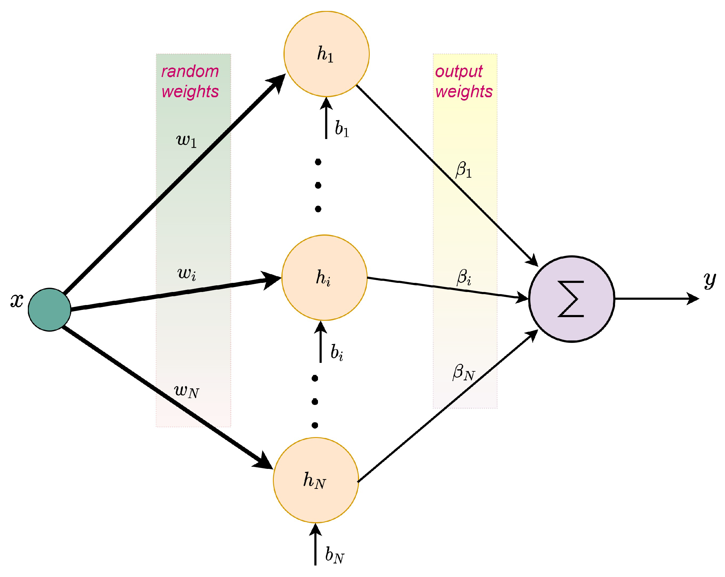
If an ideally sinusoidal flux distribution is assumed (meaning: sinusoidal radial flux density in the air gap), a motor is modeled by well-known simplified equations in the rotor oriented reference frame (notation is explained in Table 1):
L d d d t i d = ω e L q i q + ω e ψ q R s i d + V d , L q d d t i q = ω e L d i d ω e ψ d R s i q + V q .
In this case, flux-related parameters are constant:
ψ q = 0 ,   ψ d = c o n s t .
Designing a controller based on the MTPA strategy for such a simplified model is a fairly well-known task and numerous versions of this approach are described [18,19,20].
Unfortunately, in a real permanent magnet motor, the flux distribution is never perfectly sinusoidal, even if the manufacturer claims it is. Such flux distortions cause higher harmonics in no-load EMF and torque deformations. The influence of motor construction on the flux distribution, EMF, and torque are well described [21,22,23]. Especially, for interior permanent magnet motors, where the magnets are embedded inside the rotor, deformation of flux distribution is non-negligible and the simplified model (1) is unacceptable. In this case, each flux component is a non-linear function of current and rotor position [24], so a more reliable model is [25]:
L ˜ d d d t i d = ω e L q i q + ω e Ψ q ( i d , θ e ) R s i d + V d , L ˜ q d d t i q = ω e L d i d ω e Ψ d ( i d , θ e ) R s i q + V q .
The flux components Ψ q ( i q , θ e ) ,   Ψ d ( i d , θ e ) used in (3) may be complicated, non-linear functions, describing surfaces with multiple extremes.
Still, even in this situation, it is possible to minimize the losses by an MTPA approach (see, for example [26]), although it is very beneficial to have a reliable flux distribution model and to be able to compensate deformations. Having trustworthy models of flux surfaces is particularly useful in numerous applications. In addition to the energy aspect, it allows for analyzing the motor performance (torque ripples, for example) and to identify motor parameters [27,28]. They may also be used in the control loop to compensate flux and torque variations [28,29,30,31]. As analytical models obtained from field equations are too complex for practical or online applications, we concentrate on artificial neural network models.
Several methods may be used to create numerical data representing the surfaces Ψ d ( i d , θ e ) , Ψ q ( i q , θ e ) : starting from detailed 3D modeling of the motor magnetic field, ending with observers of a different type, for example, as described in [27,28,32,33]. All these methods produce data degraded (to a certain degree) by noise or outliers. An exemplary set of data is presented in Figure 1. It was obtained from a permanent magnet synchronous motor with B–202–C–21 rotor embedded permanent magnets manufactured by Kollmorgen. The diagram and the photo of the rotor are presented in Figure 2. The motor parameters are given in Table 2.
Although both flux surfaces are complex and non-linear, some regularities and repetitions are easily visible. The periodicity follows from the motor construction constant and known distance between the poles.
The shortest possible time of training is a crucial feature of a network, as the model is supposed to operate online or as a part of an embedded controller. Therefore, we decided to apply the so-called extreme learning machine (ELM) [34,35]—a neural network with activation function parameters selected at random. The most important advantage of the ELM is the extremely short training time, as training means solving a linear mean square problem and it is carried out in just one algebraic operation.
We start with a presentation of a classical ELM and discuss the effectiveness of its application to the motor flux modeling problem. Motivated by the features of this problem, having in mind the well-known drawbacks of ELMs, we present two new network structures that allow us to use the available information about the data effectively, preserving the simplicity and short training time.

3. Standard ELM

Architecture of a standard ELM is presented in Figure 3.
As was proven [34], the selection of a particular activation function (AF) is not critical for the network performance. Assuming sigmoid AFs for all hidden neurons is commonly accepted:
h i ( x ) = 1 1 + e x p ( x T w i + b i ) .
It is typical for a standard ELM approach that the weights w i = [ w i , 1 , w i , n ] T and the biases b i are selected at random, according to the uniform distribution in [ 1 , 1 ] [34,35]. The training data for an n-input ELM form a batch of M samples x k R n , k = 1 , , M and corresponding desired outputs t = [ t 1 , t M ] T . It is assumed that each input is normalized to the interval [0,1]. The batch of M samples is transformed by an ELM with N M hidden neurons into M values of output:
y = y 1 y M = h 1 , 1 h 1 , N h M , 1 h M , N β 1 β N = H β ,
where h k , i is the value of the i-th AF calculated for the k-th sample and β i is the output weight of the i-th neuron. Optimal output weights β o p t minimize the network performance index
E = β + C H β t 2 ,
hence
β o p t = 1 C I + H T H 1 H T t .
The design parameter C > 0 is introduced to avoid high condition coefficients of the matrix P : = 1 C I + H T H . This approach is called Tikhonov regularization [36,37]. A smaller value of C makes the structure of P closer to the identity matrix, but degrades the approximation accuracy, as β has a stronger impact on the performance index. A high value of C makes β o p t closer to β m i n = H + t where H + is the Moore–Penrose generalized inverse of matrix H + . The vector β m i n minimizes E 0 = H β t 2 .
A standard ELM possesses the universal approximation property [34,35,37]. This means that by increasing the number of hidden neurons, we may decrease the approximation error arbitrarily. Unfortunately, the large number of neurons increases the probability that some columns of H become almost co-linear, and generates numerical difficulties and high output weights. Tikhonov regularization is supposed to help, but it is not easy, or may even be impossible, to find a compromise value of parameter C. Several approaches to solve this dilemma were proposed (see [38,39,40] and the references therein), but none of them is perfect.
It is well recognized that insufficient variation in activation functions is responsible for numerical problems of ELMs [39,40]. Sigmoid functions with the weights and biases distributed uniformly in [−1,1] behave like linear functions in the unit hypercube and may demonstrate insignificant variation. A simple improvement was proposed in [40] and is implemented here. The first step to enlarge variation in the sigmoid activation functions is to increase the range of weights w k , i w m a x , w m a x . The weights must be large enough to expose the non-linearity of the sigmoid AF, and small enough to prevent saturation. Higher weights allow us to generate steeper surfaces and should correspond with slopes of the data.
Next, the biases are selected to guarantee that the range of each sigmoid function is sufficiently large. The minimal value of the sigmoid function h k ( x ) in the unit hypercube 0 x i 1 ,   i = 1 , , n is achieved at the vertex selected according to the following rules: w k , i > 0 x i = 0 , w k , i < 0 x i = 1 , i = 1 , , n , and equals h k , m i n = 1 1 + e x p i : w k , i < 0 w k , i + b k , while the maximum value is achieved at the vertex: w k , i > 0 x i = 1 , w k , i < 0 x i = 0 , i = 1 , , n , and equals h k , m a x = 1 1 + e x p i : w k , i > 0 w k , i + b k . Therefore, if the biases are selected at random from intervals,
b ¯ , b ˜ : = i : w k , i > 0 w k , i l n 1 r 2 1 ,   l n 1 r 1 1 i : w k , i < 0 w k , i ,
the sigmoid function h k ( x ) has a chance to cover the interval [ r 1 , r 2 ] .
This approach—enhancing variation in activation functions—is applied to model flux surfaces in all experiments presented in this paper. Still, some drawbacks of the standard ELM modeling are noticeable, therefore, we propose two new network architectures to improve the modeling quality.

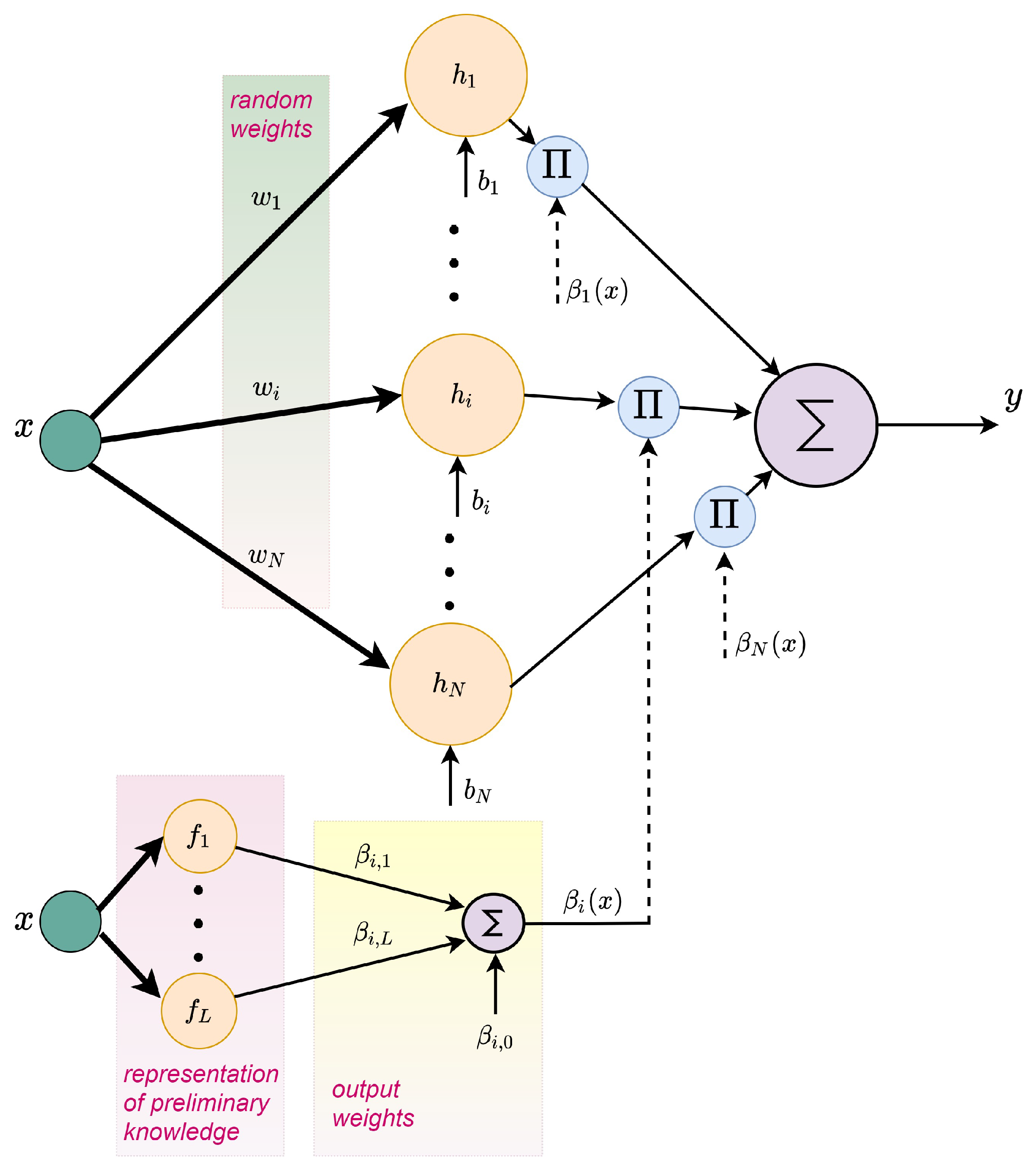
4. ELM with Input-Dependent Output Weights

4.1. New Network Structure

Very short learning times and the simplicity of the algorithm are the most attractive features of ELMs. The greatest disadvantage of a standard ELM is that a non-linear transformation with randomly selected parameters may be unable to represent all important features of the input space. Hence, a large number of neurons is necessary, which generates the numerical problems described above and in [39,40,41,42,43,44].
If we have some, even approximate, information about the structure of the modeled non-linearity, we may pass this knowledge through the network. As it is trusted information, we do not allow the network to modify it deeply. However, because it is still only partial, approximate, and incomplete knowledge, we accept a slight modification.
Motivated by this philosophy, we propose the following network structure. If we assume that L known non-linear functions of the input f l ( x ) , l = 1 , , L should be represented in the model output, we plug in those functions into the output weights β , making each weight a function of input. The network output is now given by
y = i = 1 N h i ( x ) β i ( x ) , β i ( x ) = β i , 0 + l = 1 L β i , l f l ( x ) .
The information represented in f l ( x ) , l = 1 , , L has a strong impact on the output, but it can still be modified by coefficients β i , l . The standard ELM structure is represented by the weights β i , 0 and the standard ELM is a special case of the structure presented in (9) obtained for β i , l = 0 . Therefore, the proposed network preserves the universal approximation property of the standard ELM.
Expanding Formula (9) provides
y = i = 1 N h i ( x ) β i , 0 + i = 1 N h i ( x ) f 1 ( x ) β i , 1 + + i = 1 N h i ( x ) f L ( x ) β i , L .
Architecture of the proposed ELM is presented in Figure 4.
Hence, Formula (9) is equivalent to a standard ELM structure with N ( l + 1 ) hidden neurons equipped with activation functions h i ( x ) , i = 1 , , N , h i ( x ) f 1 ( x ) , i = 1 , , N , …, h i ( x ) f L ( x ) , i = 1 , , N . Sigmoid functions h i ( x ) with randomly selected parameters represent a random, non-linear transformation of inputs into the feature space, while f l ( x ) , l = 1 , , L code an assumed knowledge about the data structure. We expect that using this knowledge directly inside the network will reduce the total number of neurons required to obtain the desired modeling accuracy, compared with a standard ELM.
A batch of M samples generates M output values
y = y 1 y M = g 1 , 1 g 1 , N ( L + 1 ) g M , 1 g M , N ( L + 1 ) β ^ = G β ^ ,
where β ^ = [ β 1 , 0 , , β N , 0 , β 1 , 1 , , β N , 1 , , β 1 , L , , β N , L ] T and g i , k are the value of the k -th function from the sequence
[ g 1 ( x ) , , g N ( L + 1 ) ( x ) ] : = [ h 1 ( x ) , , h N ( x ) , h 1 ( x ) f 1 ( x ) , , h 1 ( x ) f L ( x ) , , h N ( x ) f 1 ( x ) , , h N ( x ) f L ( x ) ]
calculated for the i-th sample. Optimal weights, minimizing the performance index E ^ = β ^ + C G β ^ t 2 , are given by
β ^ o p t = 1 C I + G T G 1 G T t .

4.2. Reduction of Output Weight Number

The coefficient h i ( x ) which multiplies each function f l ( x ) in (10) depends on the actual value of input x and randomly selected parameters of the activation function. So, to a certain degree, it is a random number from the interval [0,1]. If our aim is to simplify the network (10) and to reduce the number of output weights, while still preserving the information represented in functions f l ( x ) , we may take a random gain for each f l ( x ) and use one output weight for a group of functions f l ( x ) . For example, modification of the standard ELM according to
y = i = 1 N h i ( x ) β i ( x ) , β i ( x ) = β i , 0 + β i , 1 l = 1 L a i , l f l ( x ) ,
where parameters a i , l , l = 1 , , L are randomly selected results in
y = i = 1 N h i ( x ) β i , 0 + i = 1 N h i ( x ) l = 1 L a i , l f l ( x ) β i , 1 .
Architecture of the reduced ELM is presented in Figure 5.
Hence, (15) is equivalent to a standard ELM with 2 N hidden neurons and activation function h i ( x ) , i = 1 , , N and h i ( x ) l = 1 L a i , l f l ( x ) , i = 1 , , N . Again, the standard ELM is a special case of (15), so the network (15) possesses the universal approximation property.
Responding to the batch of M samples (15) generates M output values
y = y 1 y M = r 1 , 1 r 1 , 2 N r M , 1 r M , 2 N β ˜ = R β ˜ ,
where β ˜ = [ β 1 , 0 , , β N , 0 , β 1 , 1 , , β N , 1 ] T and r i , k are the value of the k-th function from the sequence
[ r 1 ( x ) , , r 2 N ( x ) ] : = [ h 1 ( x ) , , h N ( x ) , h 1 ( x ) l = 1 L a 1 , l f l ( x ) , , h N ( x ) l = 1 L a N , l f l ( x ) ]
calculated for the i-th sample. Optimal weights, minimizing the performance index E ˜ = β ˜ + C R β ˜ t 2 , are given by
β ˜ o p t = 1 C I + R T R 1 R T t .
Although the network (15) is simpler than (9), it is not necessarily less accurate for the same number of output weights.

5. Comparison of Networks

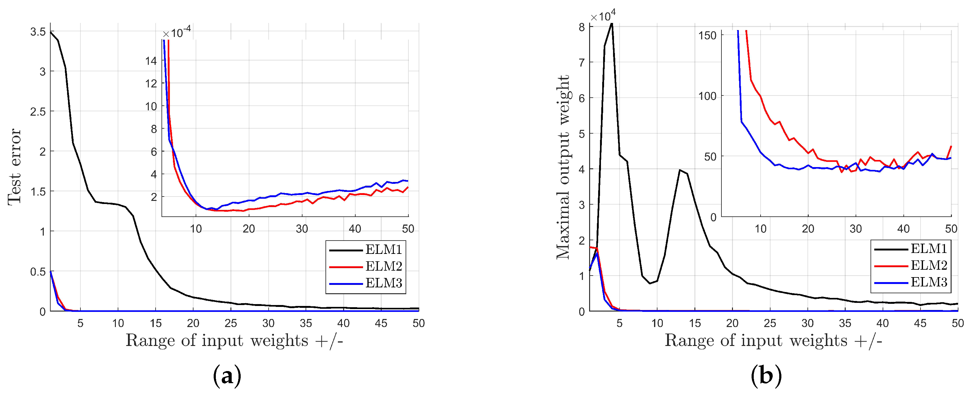
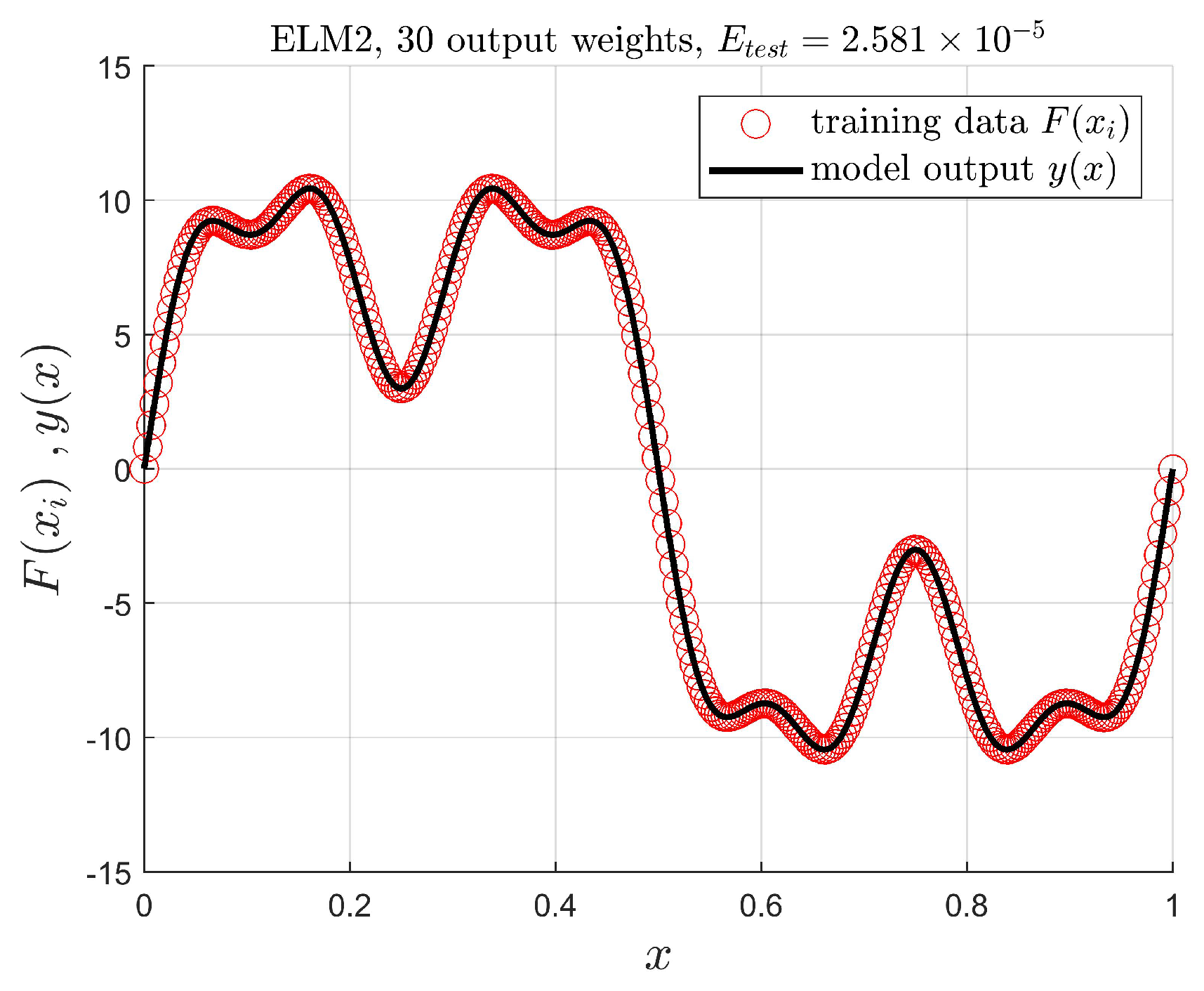
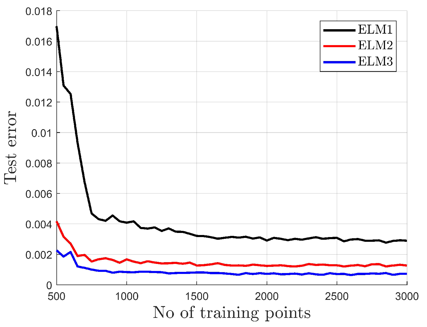
5.1. Introductory Example

To clearly demonstrate the idea of the proposed modifications, we start with a simple one-dimensional example. The curve to be approximated is given by
F ( x ) = 10 f 0 ( x ) + 5 f 1 ( x ) + 2 f 2 ( x ) = 10 sin ( 2 π x ) + 5 sin ( 6 π x ) + 2 sin ( 14 π x ) 0 x 1 .
The training set consists of N t r = 300 pairs x i , F ( x i ) where x i are equidistantly distributed in [0,1], while the test data are formed by N t e s t = 1000 such points. The final result is judged by the mean value of
E t e s t = 1 N t e s t i = 1 N t e s t F ( x i ) y ( x i ) 2 ,
where y is the model output obtained from 1000 experiments.
Three networks are compared:
  • ELM1: The standard ELM given by (5), (7) with the input weights and biases selected randomly, according to the enhanced variation mechanism (8) with r 1 = 0.1 , r 2 = 0.9 .
  • ELM2: The network with input-dependent output weights, according to (9):
    β i ( x ) = β i , 0 + β i , 1 f 1 ( x ) + β i , 2 f 2 ( x ) ,
    where the partial knowledge about the output is used.
  • ELM3: The network modified according to (14):
    β i ( x ) = β i , 0 + β i , 1 a i , 1 f 1 ( x ) + a i , 2 f 2 ( x ) ,
    where a i , 1 , a i , 2 are selected at random from the interval [−1,1].
We compare the networks with the same number of the output weights, so, if we use N hidden neurons in ELM1, the corresponding ELM2 has N / 3 , and ELM3— N / 2 neurons.
In this simple example, all three networks work properly, in the sense that we can obtain a correct approximation from any of them. An exemplary plot is presented in Figure 6. For other networks, we obtain similar results, but important differences are illustrated in Figure 7, Figure 8 and Figure 9.
Enhancement of the variance of activation functions was applied for each network. Figure 7 demonstrates that a sufficient range of input weights is important, but it also illustrates that:
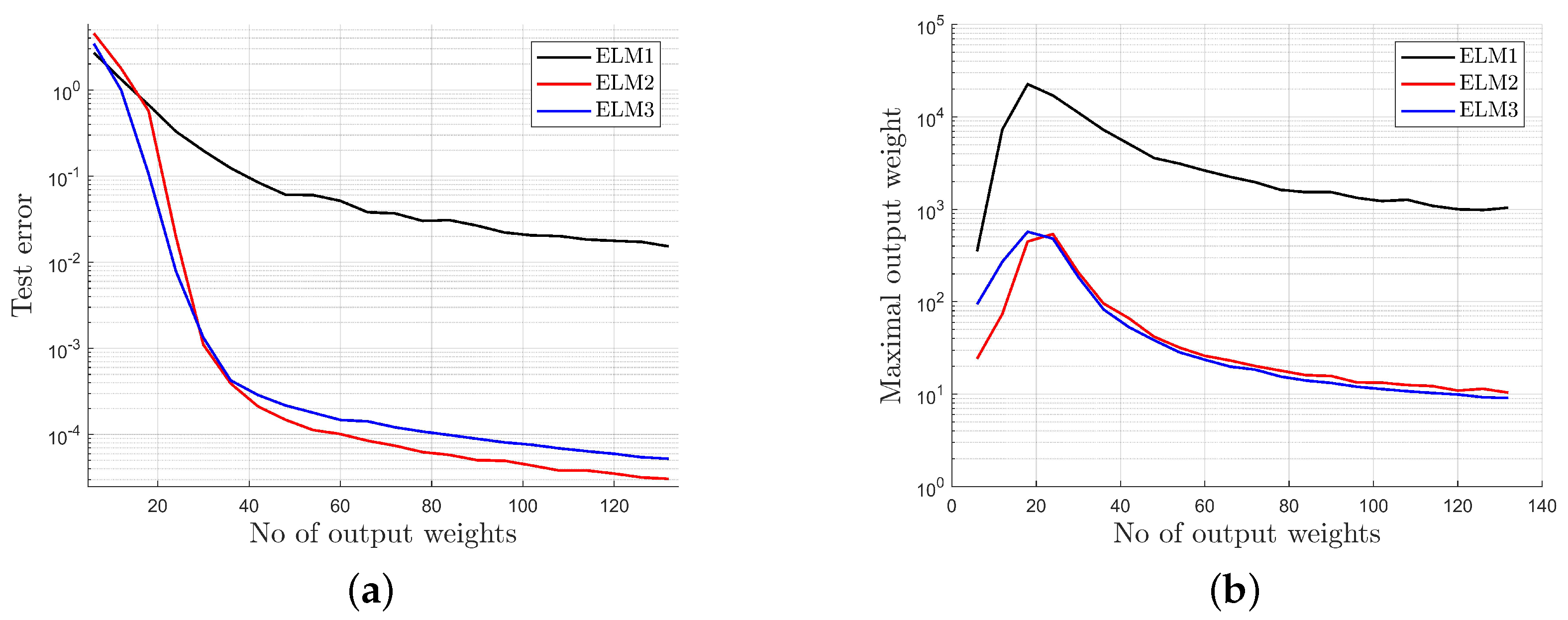
  • The standard network (ELM1) is far more sensitive to a small range of input weights than modified networks (ELM2 and ELM3).
  • The standard network (ELM1) generates a higher test error than modified networks (ELM2 and ELM3), in spite of the range of the input weights.
  • The standard network (ELM1) generates much higher output weights than modified networks (ELM2 and ELM3), so the standard model demonstrates much worse numerical properties.
The influence of the number of output weights (number of hidden neurons) is presented in Figure 8. It is shown that:
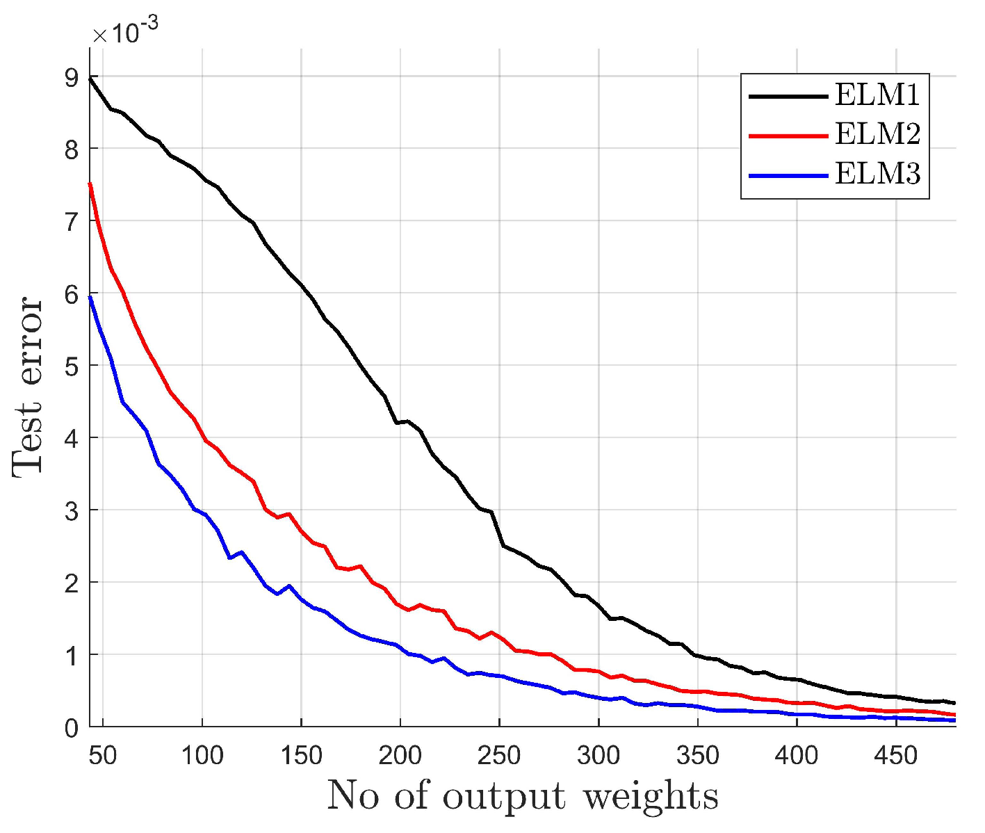
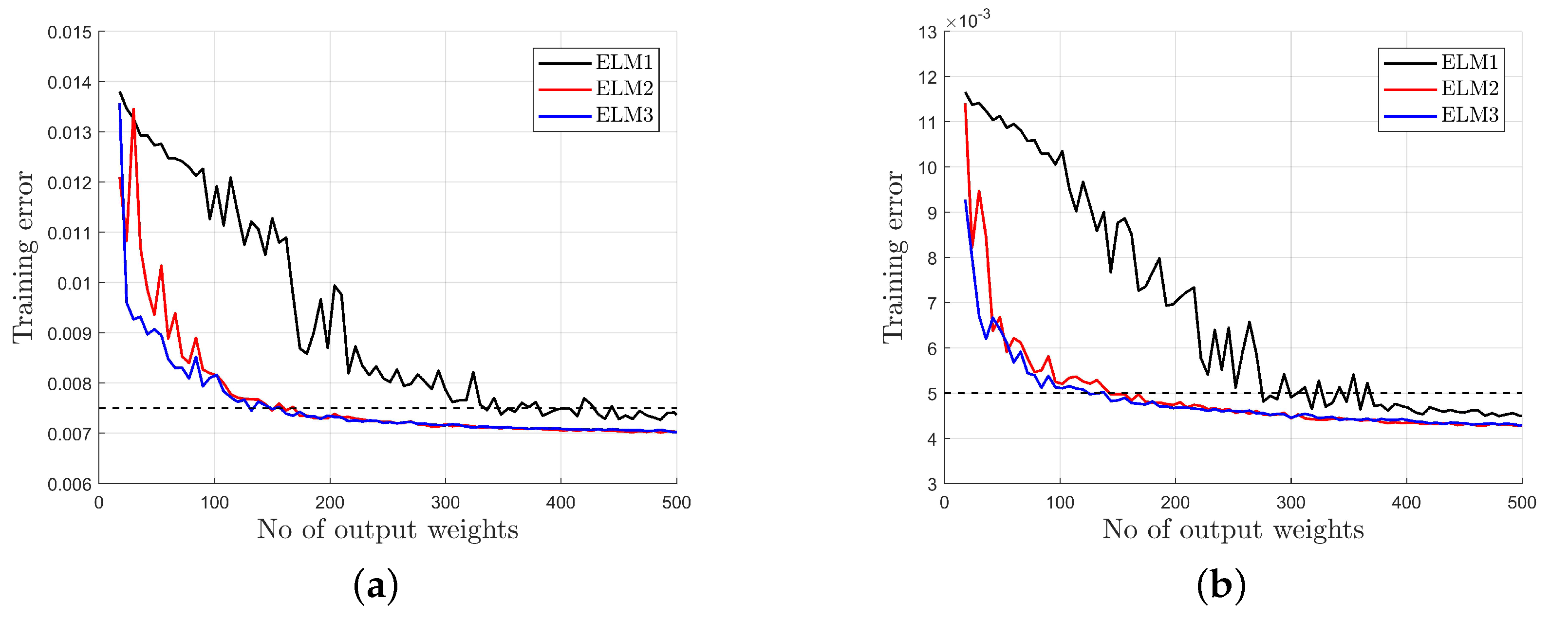
  • The standard network (ELM1) generates higher test error than modified networks (ELM2 and ELM3) for the same number of output weights and requires a much larger number of hidden neurons to obtain a similar test error as ELM2 or ELM3.
  • The standard network (ELM1) generates much higher output weights for any number of hidden neurons than modified networks (ELM2 and ELM3), so the standard model demonstrates much worse numerical properties.
The impact of the regularization parameter C is presented in Figure 9. It is evident that:
  • The standard network (ELM1) generates a much higher test error for any C than modified networks (ELM2 and ELM3).
  • The standard network (ELM1) requires strong regularization (small C to decrease output weights), resulting in poor modeling accuracy. The modified networks (ELM2, ELM3) preserve moderate output weights for any C—regularization is not necessary.

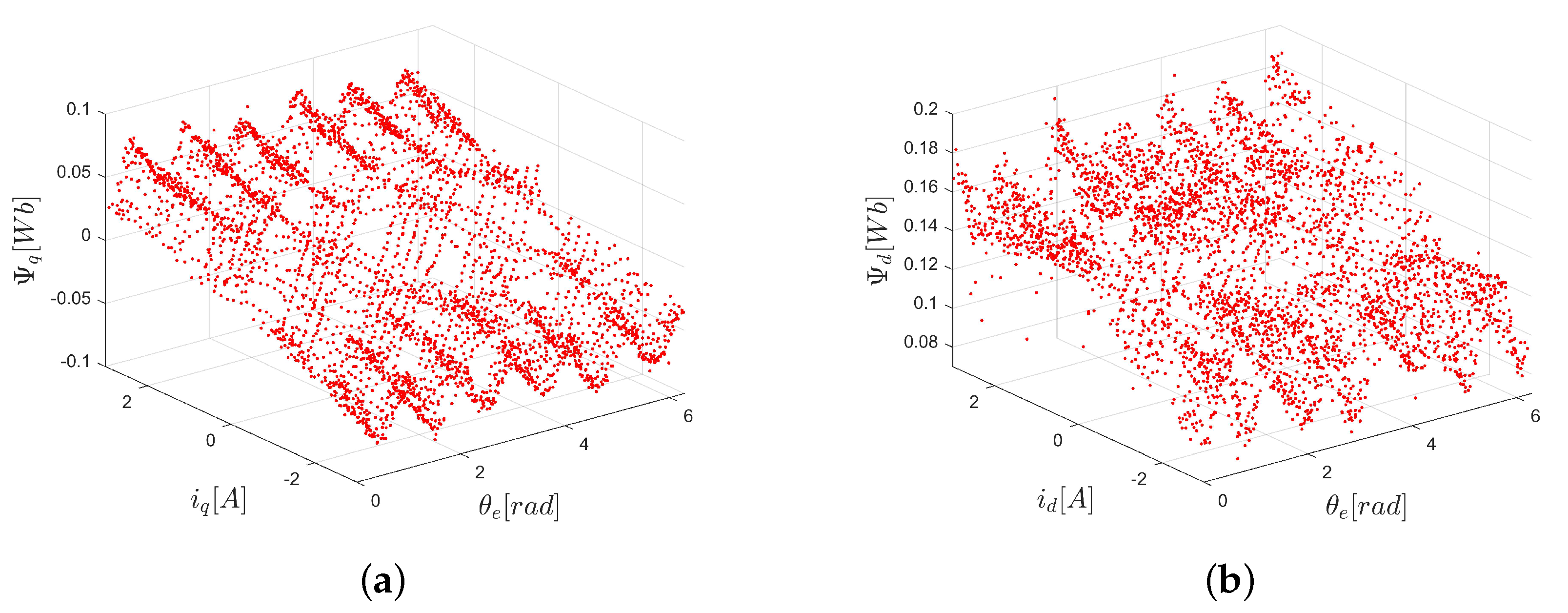
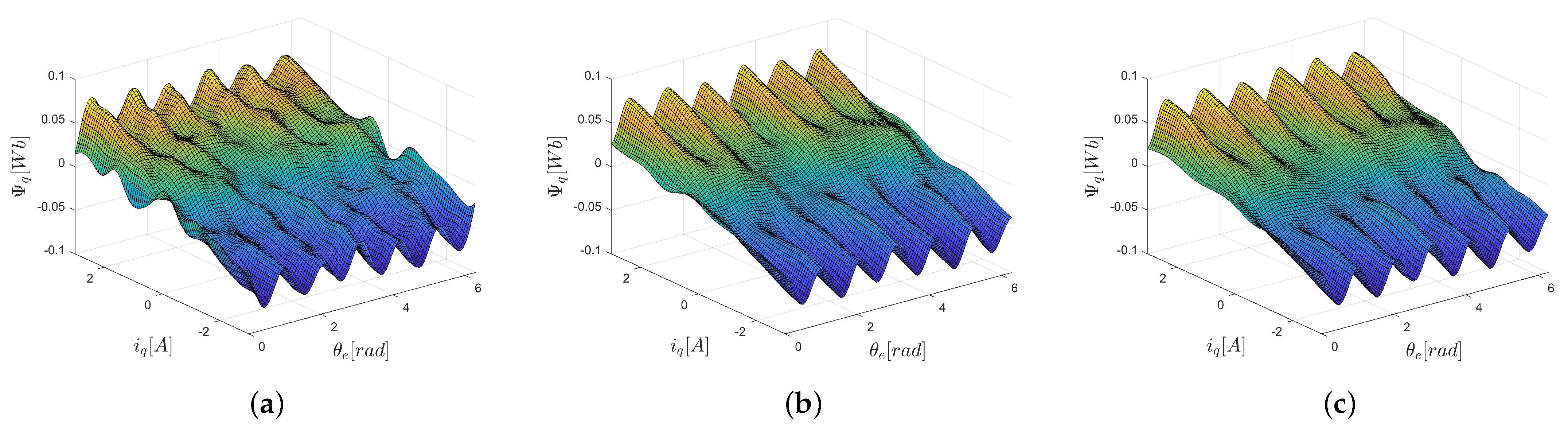
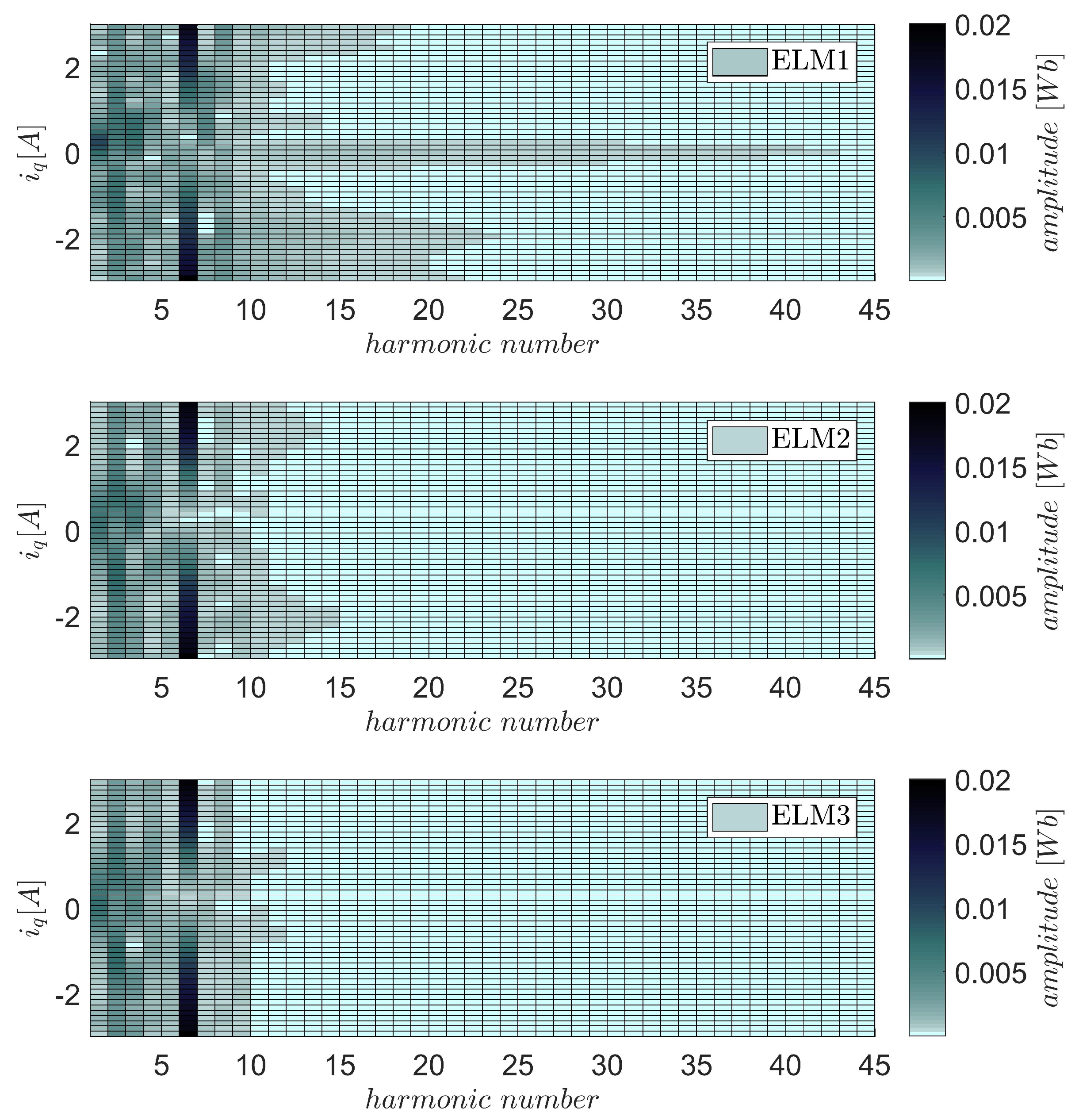
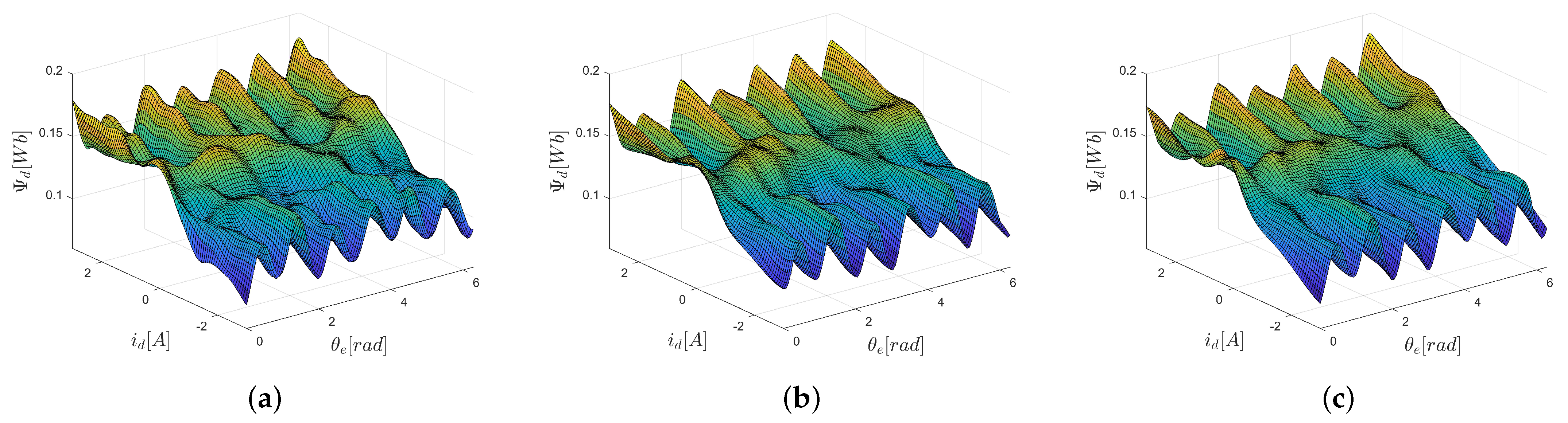
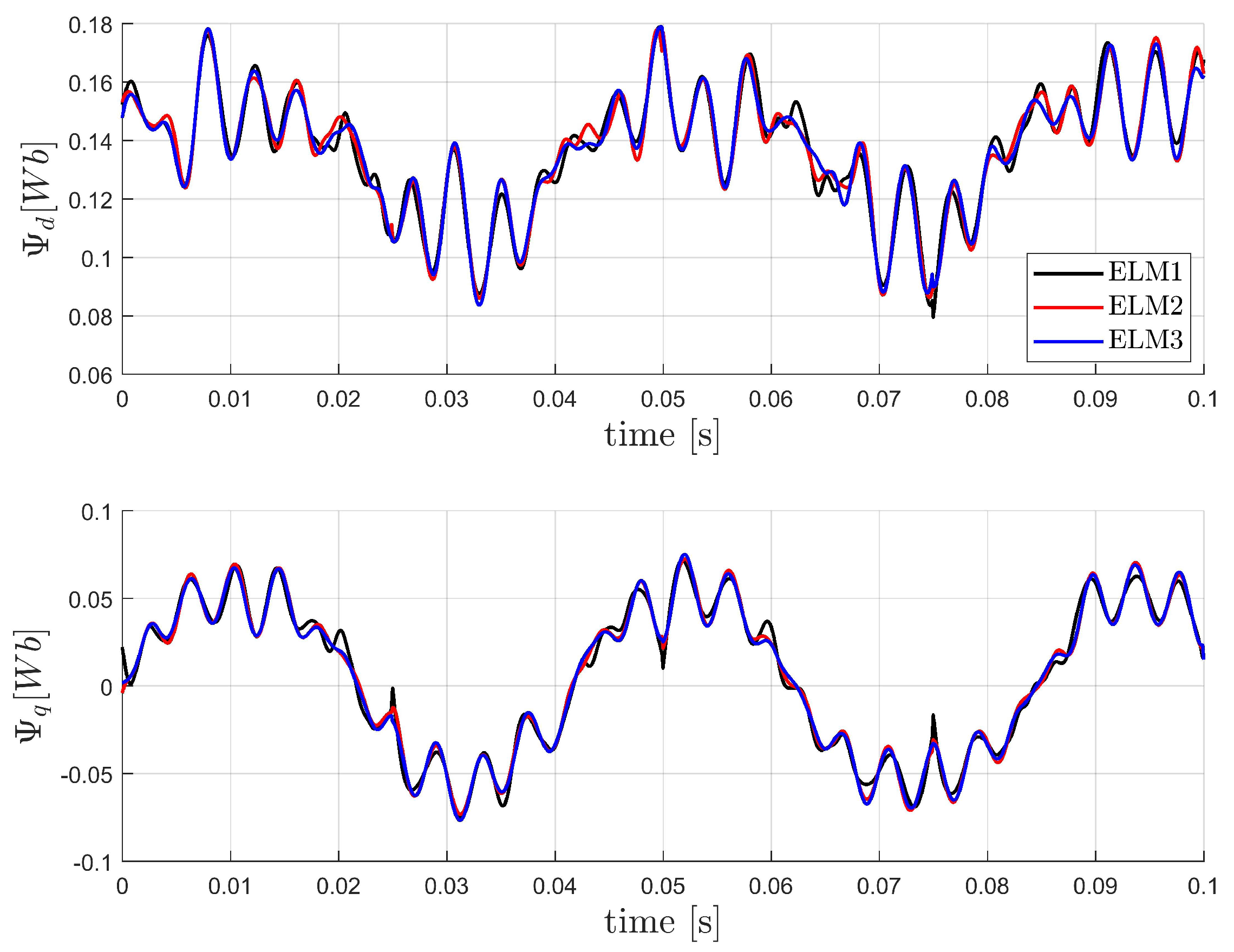
5.2. Motor Flux Modeling

To compare the performance of the discussed networks precisely, a numerically generated surface is used. The surface is presented in Figure 10, and it is similar to Ψ q ( i q , θ e ) presented in Figure 1b. The formula generating the surface is:
t ( x 1 , x 2 ) = 0.1 p 1 ( 2 x 2 1 ) + 0.02 sin ( 12 π x 1 ) ( 2 x 2 1 ) + 0.3 p 2 ( 10 x 2 5 ) , p 1 ( δ ) = 2 1 + exp ( 2 δ ) 1 ,   p 2 ( δ ) = exp ( δ ) .
Using artificial data allows us to calculate the training and test errors accurately. For each experiment, three sets of data are generated:
  • training data t i ( x 1 , i , x 2 , i ) , i = 1 , , N t r , where ( x 1 , i , x 2 , i ) are randomly selected from the input area [0,1] × [0,1],
  • training data corrupted by noise t i * ( x 1 , i , x 2 , i ) = t i ( x 1 , i , x 2 , i ) ( 1 + γ i ) , i = 1 , , N t r , where γ i is a random variable possessing normal distribution N ( 0 , 0.1 ) ,
  • testing data t i 0 ( x 1 , i 0 , x 2 , i 0 ) , i = 1 , , N t e s t randomly selected from the input area [0,1] × [0,1], different from the training data. N t e s t = 3000 is used for all experiments.
The main index used to compare the networks is the test error:
E t e s t = 1 N t e s t i = 1 N t e s t t i 0 ( x 1 , i 0 , x 2 , i 0 ) y ( x 1 , i 0 , x 2 , i 0 ) 2 ,
where y denotes the actual network output. The test error E t e s t compares the network output with accurate data, even if noisy data were used for training.
As each network depends on randomly selected parameters, 100 experiments are performed and mean values of obtained test errors are used for comparison. The average value from the modeled surface is about 0.05, so an error smaller than 0.005 provides the relative error ∼10%.
Three networks are compared:
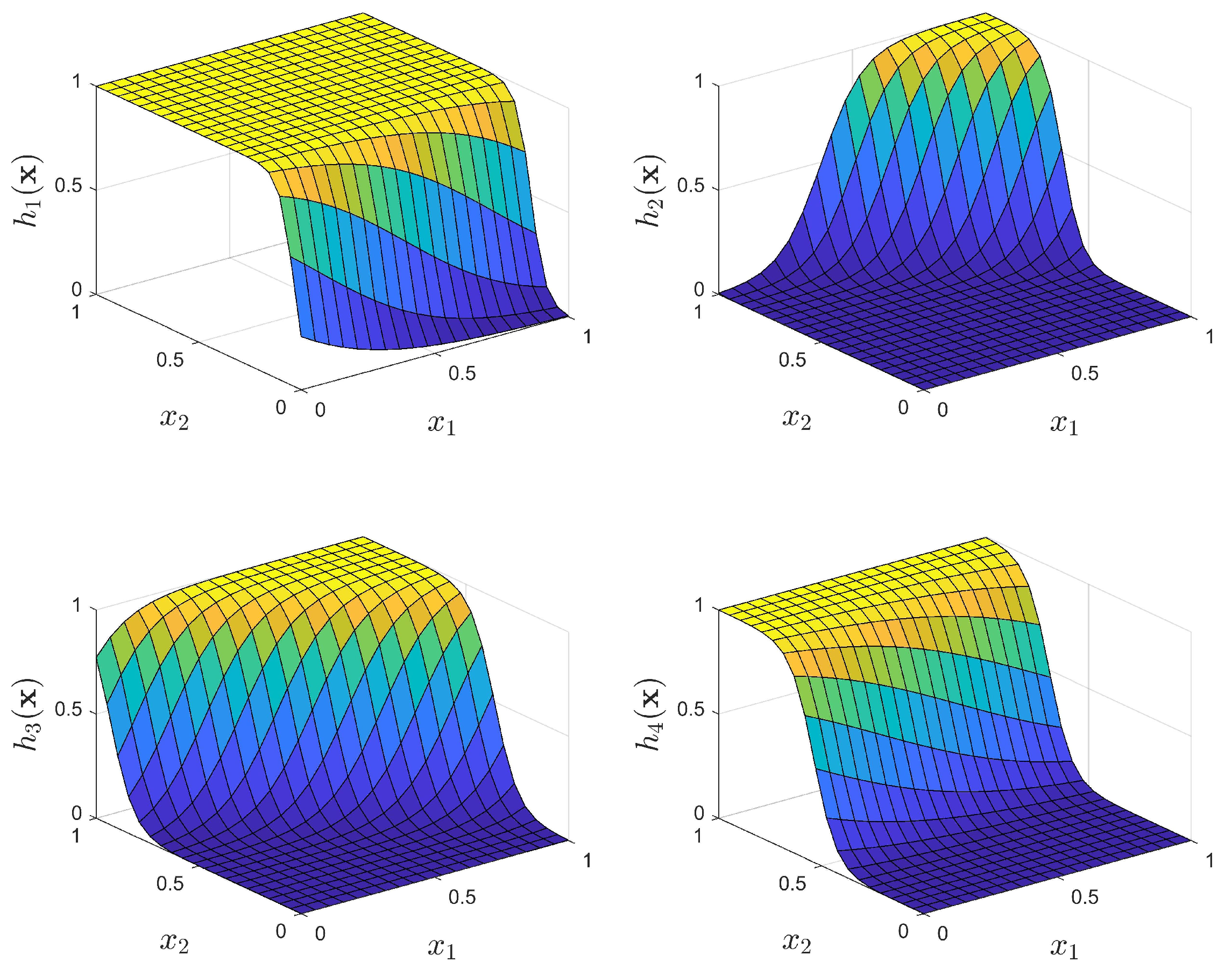
  • ELM1: The standard ELM given by (5), (7) with the input weights selected randomly, according to a uniform distribution, from the interval [ w m a x , w m a x ] = [ 30 , 30 ] and the biases selected according to (8) for r 1 = 0.1 , r 2 = 0.9 This approach provides activation functions with a sufficient variance, as presented in Figure 11.
  • ELM2: The network with input-dependent output weights, according to (9):
    β i ( x ) = β i , 0 + β i , 1 f 1 ( x ) + β i , 2 f 2 ( x ) , f 1 ( x ) = sin ( 12 π x 1 )   f 2 ( x ) = cos ( 12 π x 2 ) ,
    where the knowledge about the motor construction (number of pole pairs) is used to propose f 1 ( x ) , f 2 ( x ) .
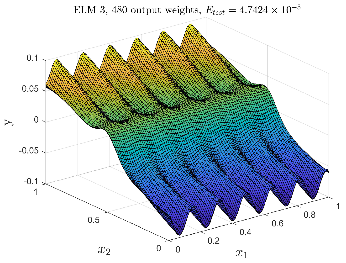
  • ELM3: The network with input-dependent output weights, according to (14):
    β i ( x ) = β i , 0 + β i , 1 a i , 1 f 1 ( x ) + a i , 2 f 2 ( x ) , f 1 ( x ) = sin ( 12 π x 1 )   f 2 ( x ) = cos ( 12 π x 2 ) ,
    where a i , 1 , a i , 2 are selected at random from interval [−1,1].
As carried out previously, we compare the networks with the same number of output weights, so if we use N hidden neurons in ELM1, the corresponding ELM2 has N / 3 , and ELM3— N / 2 neurons.
The test errors of compared networks as functions of output weight number are presented in Figure 12 for noiseless data N t r =3000 and N t e s t = 3000 , C = 10 10 , w m a x = 30 .
The modified networks (ELM2 and ELM3) provide significantly lower modeling errors than the standard one (ELM1). The surface generated by one of the modified networks is presented in Figure 13, it is indistinguishable from the original one plotted in Figure 10.
The advantage of modified networks (ELM2 and ELM3) becomes more visible when the information about the surface is poorer. Figure 14 presents the test error as the function of the number of training points N t r for N t e s t = 3000 , C = 10 10 , w m a x = 30 , N = 240 .
The modified networks also offer smaller test errors if the training data are corrupted by noise. This situation is presented in Figure 15 for N t r = 3000 and N t e s t = 3000 , C = 10 10 , w m a x = 30 . The advantage of modified networks is even more significant, as in the presence of the noisy data it is impossible to increase the number of neurons arbitrarily. A large number of hidden neurons causes an increase in the test error as the network loses generalization properties due to overfitting. The analysis of the error surface structure demonstrates that the smaller number of neurons gives a smoother modeling error surface with a smaller number of local extremes.

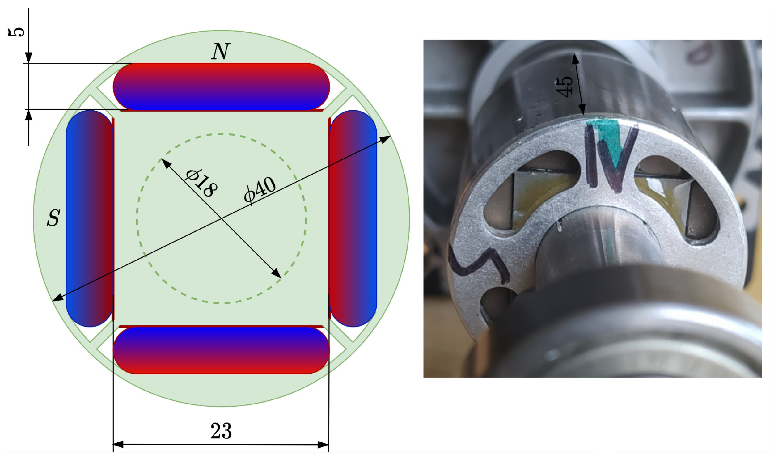
5.3. Modeling of Experimental Data

A similar comparison of the networks is repeated with the experimental data presented in Figure 1. The data set was divided into the training data N t r = 20,000 and the test data N t e s t = 20,000. Of course, as the accurate value of the flux is unknown, the test error is defined with respect to the experimental data from the test data set. The training and the test error behave similarly, so only the training error is plotted in Figure 16. The result of the comparison is similar: for both flux surfaces, the modified networks (ELM2 and ELM3) provide significantly lower modeling errors than the standard one (ELM1).
The number of hidden neurons and output weights necessary to obtain a training error smaller than 0.0075 for Ψ d ( i d , θ e ) or smaller than 0.0050 for Ψ q ( i q , θ e ) is presented in Table 3.
The surfaces generated by the networks described in Table 3 are presented in Figure 17 and Figure 18. Of course, currents and position are rescaled to the original range in amperes and radians. Application of networks ELM2 and ELM3, where the knowledge about the motor construction is used, allows us to smooth the modeled surface, to reduce the number of extremes, and to obtain a continuous transition at θ e = 0 / θ e = 2 π . The models obtained from the modified networks (ELM2 and ELM3) are more regular, with a smaller number of extremes.
The time history of the flux generated for a given current–position trajectory is presented in Figure 19. The flux obtained from the modified networks (ELM2 and ELM3) is continuous for θ e = n 2 π , while the one generated from the standard network (ELM1) is not. Therefore, the model generated from ELM1 violates physical principles of motor operation, while modified networks benefit from the knowledge coded in functions f 1 ( x ) and f 2 ( x ) included in the network.
The signal presented in Figure 19 is not periodical. It is a time history of the flux generated under variable speed and current. Therefore, Fourier analysis of this signal does not provide any useful information. Instead of this, fast Fourier transform (FFT) analysis of the outputs of the considered models obtained for a constant velocity and for several fixed values of the q-axis current is presented. In this case, the flux is a periodical function of a rotor position. The results of such an analysis, shown in Figure 20, confirm the existence of the sixth harmonic with high amplitude, which is in line with the expectations. The model created with the use of the standard network (ELM1) generates non-negligible content of higher harmonics, especially for small current values. The presence of all subsequent higher harmonics in the FFT of the output of ELM1 demonstrates an undesirable ability to generate noise by this model. The modified networks ELM2 and ELM3 generate waveforms with a lower content of higher harmonics, which is undoubtedly an advantage.
Finally, a practical, hardware implementation of the proposed networks was considered. The time necessary for model execution on some popular DSP boards is presented in Table 4. The obtained results encourage the implementation of ELMs in control algorithms.

6. Conclusions

Both proposed modified structures of the ELM allow for incorporating preliminary, partial, imprecise information about modeled data into the network structure. It was demonstrated that the modified network may be interpreted as a network with input-dependent output weights, or as a network with modified activation functions. The proposed approach preserves all the attractive features of the standard ELM:
  • the universal approximation property,
  • fast, random selection of parameters of activation functions,
  • extremely short learning time, as learning is not an iterative process, but is reduced to a single algebraic operation.
It was demonstrated by numerical examples that both modified networks outperform the standard ELM:
  • offering better modeling accuracy for the same number of output weights and a smaller number of parameters, while assuring the same accuracy, therefore reducing the problem of dimensionality,
  • generating lower output weights and better numerical conditioning of output weight calculation,
  • being more flexible for Tikhonov regularization,
  • being more robust against data noise,
  • being more robust against small training data sets.
It is difficult to decide which of the proposed modifications is “better”. For the presented examples, they are comparable and the selection of one of them depends on the specific features of a particular problem.
It was shown that the proposed modified ELMs are suitable for modeling motor flux versus position and current, especially for interior permanent magnet motors. The modeling methodology was presented. The extra information about flux surfaces is available from the motor construction (pole pitch) and may be easily included. The obtained models preserve flux continuity around the rotor, and provide good agreement with measured signals (like torque and EMF), so they may be considered trustworthy.
The modified networks provide significantly lower modeling errors than the standard one and this feature becomes more visible when the information about the surface is poorer (fewer samples are available), or the training data are corrupted by noise. FFT analysis of the networks’ periodical outputs demonstrates that the modified networks generate more reliable spectra, corresponding to theoretical expectations, while the standard one generates a visible amount of high-harmonic noise.
The obtained neural models may be used for control or identification, working online. The execution times obtained from well-known DSP boards are short enough for modern algorithms of electric drive control. Therefore, we claim that the recent control methods of PMSM drives might be improved by taking flux deformations into account.

Author Contributions

Conceptualization, M.J.; methodology, M.J. and J.K.; formal analysis, M.J. and J.K.; writing—original draft preparation, M.J. and J.K.; writing—review and editing, M.J. and J.K. All authors have read and agreed to the published version of the manuscript.

Funding

The APC was funded by Lodz University of Technology.

Institutional Review Board Statement

Not applicable.

Informed Consent Statement

Not applicable.

Acknowledgments

The authors are grateful to Tomasz Sobieraj for his support in obtaining experimental data.

Conflicts of Interest

The authors declare no conflict of interest.

References

  1. Waide, P.; Brunner, C.U. Energy-Efficiency Policy Opportunities for Electric Motor-Driven Systems; International Energy Agency: Paris, France, 2011; 132p. [Google Scholar] [CrossRef]
  2. Melfi, M.J.; Rogers, S.D.; Evon, S.; Martin, B. Permanent Magnet Motors for Energy Savings in Industrial Applications. In Proceedings of the 2006 Record of Conference Papers—IEEE Industry Applications Society 53rd Annual Petroleum and Chemical Industry Conference, Philadelphia, PA, USA, 11–15 September 2006; pp. 1–8. [Google Scholar] [CrossRef]
  3. Baek, S.K.; Oh, H.K.; Park, J.H.; Shin, Y.J.; Kim, S.W. Evaluation of Efficient Operation for Electromechanical Brake Using Maximum Torque per Ampere Control. Energies 2019, 12, 1869. [Google Scholar] [CrossRef] [Green Version]
  4. Tochenko, O. Energy Efficient Speed Control of Interior Permanent Magnet Synchronous Motor. In Applied Modern Control; IntechOpen: London, UK, 2019. [Google Scholar] [CrossRef] [Green Version]
  5. Mellor, P.; Wrobel, R.; Holliday, D. A Computationally Efficient Iron Loss Model for Brushless AC Machines That Caters for Rated Flux and Field Weakened Operation. In Proceedings of the 2009 IEEE International Electric Machines and Drives Conference, Miami, FL, USA, 3–6 May 2009; pp. 490–494. [Google Scholar] [CrossRef]
  6. Tseng, K.; Wee, S. Analysis of Flux Distribution and Core Losses in Interior Permanent Magnet Motor. IEEE Trans. Energy Convers. 1999, 14, 969–975. [Google Scholar] [CrossRef]
  7. Chakkarapani, K.; Thangavelu, T.; Dharmalingam, K.; Thandavarayan, P. Multiobjective Design Optimization and Analysis of Magnetic Flux Distribution for Slotless Permanent Magnet Brushless DC motor using evolutionary algorithms. J. Magn. Magn. Mater. 2019, 476, 524–537. [Google Scholar] [CrossRef]
  8. Lee, J.G.; Lim, D.K. A Stepwise Optimal Design Applied to an Interior Permanent Magnet Synchronous Motor for Electric Vehicle Traction Applications. IEEE Access 2021, 9, 115090–115099. [Google Scholar] [CrossRef]
  9. Liang, P.; Pei, Y.; Chai, F.; Zhao, K. Analytical Calculation of D- and Q-axis Inductance for Interior Permanent Magnet Motors Based on Winding Function Theory. Energies 2016, 9, 580. [Google Scholar] [CrossRef] [Green Version]
  10. Michalski, T.; Acosta-Cambranis, F.; Romeral, L.; Zaragoza, J. Multiphase PMSM and PMaSynRM Flux Map Model with Space Harmonics and Multiple Plane Cross Harmonic Saturation. In Proceedings of the IECON 2019—45th Annual Conference of the IEEE Industrial Electronics Society, Lisbon, Portugal, 14–17 October 2019; Volume 1, pp. 1210–1215. [Google Scholar] [CrossRef]
  11. Hua, W.; Cheng, M.; Zhu, Z.Q.; Howe, D. Analysis and Optimization of Back EMF Waveform of a Flux-Switching Permanent Magnet Motor. IEEE Trans. Energy Convers. 2008, 23, 727–733. [Google Scholar] [CrossRef]
  12. Khan, A.A.; Kress, M.J. Identification of Permanent Magnet Synchronous Motor Parameters. In Proceedings of the WCX™ 17: SAE World Congress Experience, Detroit, MI, USA, 4–6 April 2017; SAE International: Warrendale, PA, USA, 2017. [Google Scholar] [CrossRef]
  13. Kumar, P.; Bhaskar, D.V.; Muduli, U.R.; Beig, A.R.; Behera, R.K. Disturbance Observer based Sensorless Predictive Control for High Performance PMBLDCM Drive Considering Iron Loss. IEEE Trans. Ind. Electron. 2021. [Google Scholar] [CrossRef]
  14. Rehman, A.U.; Choi, H.H.; Jung, J.W. An Optimal Direct Torque Control Strategy for Surface-Mounted Permanent Magnet Synchronous Motor Drives. IEEE Trans. Ind. Inform. 2021, 17, 7390–7400. [Google Scholar] [CrossRef]
  15. Jastrzębski, M.; Kabziński, J.; Mosiołek, P. Adaptive and Robust Motion Control in Presence of LuGre-type Friction. In Proceedings of the 2017 22nd International Conference on Methods and Models in Automation and Robotics (MMAR), Miedzyzdroje, Poland, 28–31 August 2017; pp. 113–118. [Google Scholar] [CrossRef]
  16. Kabziński, J.; Orłowska-Kowalska, T.; Sikorski, A.; Bartoszewicz, A. Adaptive, Predictive and Neural Approaches in Drive Automation and Control of Power Converters. Bull. Pol. Acad. Sci. Tech. Sci. 2020, 68, 959–962. [Google Scholar] [CrossRef]
  17. Kabziński, J. Advanced Control of Electrical Drives and Power Electronic Converters; Springer: Cham, Switzerland, 2017. [Google Scholar] [CrossRef]
  18. Sun, J.; Lin, C.; Xing, J.; Jiang, X. Online MTPA Trajectory Tracking of IPMSM Based on a Novel Torque Control Strategy. Energies 2019, 12, 3261. [Google Scholar] [CrossRef] [Green Version]
  19. Dianov, A.; Anuchin, A. Adaptive Maximum Torque per Ampere Control of Sensorless Permanent Magnet Motor Drives. Energies 2020, 13, 5071. [Google Scholar] [CrossRef]
  20. Zhou, Z.; Gu, X.; Wang, Z.; Zhang, G.; Geng, Q. An Improved Torque Control Strategy of PMSM Drive Considering On-Line MTPA Operation. Energies 2019, 12, 2951. [Google Scholar] [CrossRef] [Green Version]
  21. Yoon, K.Y.; Baek, S.W. Performance Improvement of Concentrated-Flux Type IPM PMSM Motor with Flared-Shape Magnet Arrangement. Appl. Sci. 2020, 10, 6061. [Google Scholar] [CrossRef]
  22. Huynh, T.A.; Hsieh, M.F. Performance Analysis of Permanent Magnet Motors for Electric Vehicles (EV) Traction Considering Driving Cycles. Energies 2018, 11, 1385. [Google Scholar] [CrossRef] [Green Version]
  23. Jang, H.; Kim, H.; Liu, H.C.; Lee, H.J.; Lee, J. Investigation on the Torque Ripple Reduction Method of a Hybrid Electric Vehicle Motor. Energies 2021, 14, 1413. [Google Scholar] [CrossRef]
  24. Krishnan, R. Permanent Magnet Synchronous and Brushless DC Motor Drives; CRC Press: Boca Raton, FL, USA, 2010. [Google Scholar]
  25. Kabzinski, J. Fuzzy Modeling of Disturbance Torques/Forces in Rotational/Linear Interior Permanent Magnet Synchronous Motors. In Proceedings of the 2005 European Conference on Power Electronics and Applications, Dresden, Germany, 11–14 September 2005; p. 10. [Google Scholar] [CrossRef]
  26. De Castro, A.G.; Guazzelli, P.R.U.; Lumertz, M.M.; de Oliveira, C.M.R.; de Paula, G.T.; Monteiro, J.R.B.A. Novel MTPA Approach for IPMSM with Non-Sinusoidal Back-EMF. In Proceedings of the 2019 IEEE 15th Brazilian Power Electronics Conference and 5th IEEE Southern Power Electronics Conference (COBEP/SPEC), Santos, Brazil, 1–4 December 2019; pp. 1–6. [Google Scholar] [CrossRef]
  27. Lin, H.; Hwang, K.Y.; Kwon, B.I. An Improved Flux Observer for Sensorless Permanent Magnet Synchronous Motor Drives with Parameter Identification. J. Electr. Eng. Technol. 2013, 8, 516–523. [Google Scholar] [CrossRef] [Green Version]
  28. Sobieraj, T. Selection of the Parameters for the Optimal Control Strategy for Permanent-Magnet Synchronous Motor. Prz. Elektrotech. 2018, 94, 91–94. [Google Scholar] [CrossRef]
  29. Wójcik, A.; Pajchrowski, T. Application of Iterative Learning Control for Ripple Torque Compensation in PMSM Drive. Arch. Electr. Eng. 2019, 68, 309–324. [Google Scholar] [CrossRef]
  30. Mosiołek, P. Sterowanie Adaptacyjne Silnikiem PMSM z Dowolnym Rozkładem Strumienia. Prz. Elektrotech. 2014, 90, 103–108. [Google Scholar] [CrossRef]
  31. Kabziński, J. Oscillations and Friction Compensation in Two-Mass Drive System with Flexible Shaft by Command Filtered Adaptive Backstepping. IFAC-Pap. 2015, 48, 307–312. [Google Scholar] [CrossRef]
  32. Veeser, F.; Braun, T.; Kiltz, L.; Reuter, J. Nonlinear Modelling, Flatness-Based Current Control, and Torque Ripple Compensation for Interior Permanent Magnet Synchronous Machines. Energies 2021, 14, 1590. [Google Scholar] [CrossRef]
  33. Kabziński, J.; Sobieraj, T. Auto-Tuning of Permanent Magnet Motor Drives with Observer Based Parameter Identifiers. In Proceedings of the 10th International Conference on Power Electronics and Motion Control, Dubrovnik & Cavtat, Croatia, 9–11 September 2002. [Google Scholar]
  34. Huang, G.B.; Zhu, Q.Y.; Siew, C.K. Extreme Larning Machine: Theory and Applications. Neurocomputing 2006, 70, 489–501. [Google Scholar] [CrossRef]
  35. Huang, G.B.; Zhou, H.; Ding, X.; Zhang, R. Extreme Learning Machine for Regression and Multiclass Classification. IEEE Trans. Syst. Man Cybern. Part B (Cybern.) 2012, 42, 513–529. [Google Scholar] [CrossRef] [PubMed] [Green Version]
  36. Tikhonov, A.N.; Goncharsky, A.V.; Stepanov, V.V.; Yagola, A.G. Numerical Methods for the Solution of Ill-Posed Problems; Springer: Dordrecht, The Netherlands, 1995. [Google Scholar] [CrossRef]
  37. Huang, G.; Huang, G.B.; Song, S.; You, K. Trends in Extreme Learning Machines: A Review. Neural Netw. 2015, 61, 32–48. [Google Scholar] [CrossRef] [PubMed]
  38. Kabziński, J. Rank-Revealing Orthogonal Decomposition in Extreme Learning Machine Design. In Artificial Neural Networks and Machine Learning—ICANN 2018; Kůrková, V., Manolopoulos, Y., Hammer, B., Iliadis, L., Maglogiannis, I., Eds.; Springer International Publishing: Cham, Switzerland, 2018; pp. 3–13. [Google Scholar]
  39. Akusok, A.; Björk, K.M.; Miche, Y.; Lendasse, A. High-Performance Extreme Learning Machines: A Complete Toolbox for Big Data Applications. IEEE Access 2015, 3, 1011–1025. [Google Scholar] [CrossRef]
  40. Kabziński, J. Extreme learning machine with diversified neurons. In Proceedings of the 2016 IEEE 17th International Symposium on Computational Intelligence and Informatics (CINTI), Budapest, Hungary, 17–19 November 2016; pp. 000181–000186. [Google Scholar] [CrossRef]
  41. Miche, Y.; Sorjamaa, A.; Bas, P.; Simula, O.; Jutten, C.; Lendasse, A. OP-ELM: Optimally Pruned Extreme Learning Machine. IEEE Trans. Neural Netw. 2010, 21, 158–162. [Google Scholar] [CrossRef] [PubMed]
  42. Feng, G.; Lan, Y.; Zhang, X.; Qian, Z. Dynamic Adjustment of Hidden Node Parameters for Extreme Learning Machine. IEEE Trans. Cybern. 2015, 45, 279–288. [Google Scholar] [CrossRef]
  43. Miche, Y.; van Heeswijk, M.; Bas, P.; Simula, O.; Lendasse, A. TROP-ELM: A Double-Regularized ELM Using LARS and Tikhonov Regularization. Neurocomputing 2011, 74, 2413–2421. [Google Scholar] [CrossRef]
  44. Parviainen, E.; Riihimäki, J. A Connection Between Extreme Learning Machine and Neural Network Kernel. Commun. Comput. Inf. Sci. 2013, 272, 122–135. [Google Scholar] [CrossRef]
Figure 1. Example of flux surfaces: (a) Ψ d ( i d , θ e ) , (b) Ψ q ( i q , θ e ) . Data collected from an identification experiment.
Energies 14 05619 g001
Figure 2. The rotor of the motor used in the experiment. Dimensions in millimeters.
Energies 14 05619 g002
Figure 3. Architecture of a standard ELM.
Energies 14 05619 g003
Figure 4. Architecture of an ELM with input-dependent output weights.
Energies 14 05619 g004
Figure 5. Architecture of a reduced ELM with input-dependent output weights.
Energies 14 05619 g005
Figure 6. The modeled curve and the network response.
Energies 14 05619 g006
Figure 7. Test error (a) and the biggest output weight (b) as a function of the range of input weights. N = 48 , C = 10 8 .
Energies 14 05619 g007
Figure 8. Test error (a) and the biggest output weight (b) as a function of the number of output weights. w m a x = 30 , C = 10 8 .
Energies 14 05619 g008
Figure 9. Test error (a) and the biggest output weight (b) as a function of the regularization coefficient C. w m a x = 30 , N = 48 .
Energies 14 05619 g009
Figure 10. The flux-like surface.
Energies 14 05619 g010
Figure 11. Exemplary activation functions of ELM1.
Energies 14 05619 g011
Figure 12. Test error as a function of the number of output weights.
Energies 14 05619 g012
Figure 13. The surface generated by one of the modified networks.
Energies 14 05619 g013
Figure 14. Test error as a function of the number of training points.
Energies 14 05619 g014
Figure 15. Test error as a function of the number of output weights. The training data corrupted by noise.
Energies 14 05619 g015
Figure 16. Modeling of: (a) Ψ d ( i d , θ e ) and (b) Ψ q ( i q , θ e ) . Training error as a function of the number of output weights.
Energies 14 05619 g016
Figure 17. Models of Ψ d ( i d , θ e ) generated by: (a) ELM1, (b) ELM2, (c) ELM3.
Energies 14 05619 g017
Figure 18. Models of Ψ q ( i q , θ e ) generated by: (a) ELM1, (b) ELM2, (c) ELM3.
Energies 14 05619 g018
Figure 19. The time history of the flux generated for a given current–position trajectory.
Energies 14 05619 g019
Figure 20. Amplitude of harmonics in q-axis flux generated from models ELM1–3 for a constant speed and several constant values of q-axis current.
Energies 14 05619 g020
Table 1. Signals and parameters in permanent magnet motor model.
NotationSignal/ParameterUnit
L d d-axis inductance[H]
L q q-axis inductance[H]
R s phase resistance[ Ω ]
ψ d , ψ q d and q permanent magnet flux components[Vs/rad]
Ψ d = Ψ d i + ψ d d current dependant and magnet flux components[Vs/rad]
Ψ q = Ψ q i + ψ q q current dependant and magnet flux components[Vs/rad]
L ˜ d = δ δ i d Ψ d i d flux derivative with respect to currents[H]
L ˜ q = δ δ i q Ψ q i q flux derivative with respect to currents[H]
θ e electric rotor position[rad]
ω e = d d t θ e electric rotor velocity[rad/s]
V d , V q d- and q-axis voltages[V]
Table 2. Motor parameters.
NotationSignal/Parameter
Rated power1.5 kW
Rated velocity6200 r/min
Rated torque2.59 Nm
Rated current5 A
Inertia 10 5 kgm 2
EMF constant0.1147 Vs
Torque constant0.49 Nm/ARMS
Phase resistance2.34 Ω
Phase inductance25 mH
Table 3. Number of hidden neurons and output weights necessary to obtain the desired training error value.
Axis ELM1ELM2ELM3
qNo of hidden neurons3365064
No of output weights336150128
dNo of hidden neurons2764863
No of output weights276144126
Table 4. Time necessary for model execution.
DSP BoardELM1ELM2ELM3
DS1104470 μ s70 μ s70 μ s
DS100630 μ s12 μ s12 μ s
Publisher’s Note: MDPI stays neutral with regard to jurisdictional claims in published maps and institutional affiliations.

