Krasovskii Passivity and μ-Synthesis Controller Design for Quasi-Linear Affine Systems

Abstract

This paper presents an end-to-end method to design passivity-based controllers (PBC) for a class of input-affine nonlinear systems, named quasi-linear affine. The approach is developed using Krasovskii’s method to design a Lyapunov function for studying the asymptotic stability, and a sufficient condition to construct a storage function is given, along with a supply-rate function. The linear fractional transformation interconnection between the nonlinear system and the Krasovskii PBC (K-PBC) results in a system which manages to follow the provided input trajectory. However, given that the input and output of the closed-loop system do not have the same physical significance, a path planning is mandatory. For the path planning component, we propose a robust controller designed using the $\mu$-synthesis mixed-sensitivity loop-shaping for the linearized system around a desired equilibrium point. As a case study, we present the proposed methodology for DC-DC converters in a unified manner, giving sufficient conditions for such systems to be Krasovskii passive in terms of Linear Matrix Inequalities (LMIs), along with the possibility to compute both the K-PBC and robust controller alike.

1. Introduction

In the recent years, passivity theory has gained renewed attention because of its advantages and practicality in modelling of multi-domain systems and constructive control techniques. Starting with the classical theory of dissipative systems of [1,2], the idea of differential passivity based on the idea of variational systems was developed in [3,4]. The same authors extended in [5] the idea to the incremental passivity concept. More recently, the idea of Krasovskii’s passivity was developed in [6]. This approach is based on the construction of a storage function using Krasovskii’s method to design a Lyapunov candidate function for stability as in [2]. Moreover, all these methods are useful for designing a simpler and more robust passivity-based controller (PBC).

However, a PBC manages to guarantee the closed-loop stability and reference tracking in terms of the command signal. But, in many cases, systems do not have the same physical significance and relevance for both input and output signals and, as such, an additional path planning procedure is necessary. For the purpose of this paper, we propose a robust controller to play this role, because robustness represents a major problem studied in Control Theory, with high impact in the literature, encompassing the sensitivity of a system with respect to both internal and external disturbances. The classical solutions for robust control problems uses ${\mathcal{H}}_2$ and ${\mathcal{H}}_{\infty }$ norms as a performance measure. The most common approaches to solve such problems are Algebraic Riccati Equations (AREs) [7] and Algebraic Riccati Inequalities (ARIs) [8]. In order to solve AREs in a more numerically stable manner, a solution using Popov triplets was presented in [9]. An open-source implementation of the above method is presented in [10], along with an iterative refinement described in [11]. In order to overcome the limitations of the ARE-based solutions, consisting in the impossibility of solving singular problems, a Linear Matrix Inequality (LMI) based solution was developed in [12]. For solving robust and nonlinear control problems using LMIs, an open-source implementation is described in [13]. Moreover, an open-source toolbox for automatically modelling uncertainties as required in robust control problems using MATLAB is presented in the paper [14].

Nowadays, renewable energy sources play an increasingly important role in the energy conversion, due to the negative consequences of the global warming. DC-DC converters have been found to be an adequate solution regarding renewable energy harvesting such as for sustaining prescribed voltages for high-power loads and for maximum power point tracking, as in [15,16,17], or in DC microgrids, as in [18]. An interior point method for renewable energy management was introduced in [19], where the importance of the good performance in the DC-DC converters control is underlined. For modelling DC-DC converters, there are two major improvements: the averaging of ON and OFF state-space models from [20], obtaining a nonlinear model, along with adding parasitic components in the circuit model, such as series and parallel resistors in the switching elements and passive components alike, as in [21]. The average model greatly simplifies the computations and well approximates the physical switching system to a desired ripple tolerance, based on the PWM period. Using these ideas, a technique which adds a damping injection term to reach the passivity of the system was presented in [22], and was extended for the nonideal DC-DC boost converter in [23]. A Krasovskii passive proportional-integral (PI) type controller was designed for the ideal case of DC-DC converters in [6].

The main contributions of the current paper are: a mathematical framework for studying the property of quasi-linear input-affine nonlinear systems to be passive, a method to design a passivity-based controller for such a nonlinear systems, along with an entire software mechanism which manages to compute both PBC and robust controllers. First, we provide an extended set of sufficient conditions for a quasi-linear input-affine nonlinear system to be Krasovskii passive, along with a set of necessary and sufficient conditions for DC-DC buck, boost and single-ended primary inductor (SEPIC) converters to construct an output such that the systems are Krasovskii passive. These extended methods can be used even for nonideal converters, compared to the sufficient set of conditions presented in [6]. Also, we present a method to design a Krasovskii passivity-based controller (K-PBC) which, along with the output port variable of the DC-DC converter, manages to ensure the closed-loop stability. This means that the lower linear fractional transformation between the system and the controller is asymptotically stable and manages to track any provided input trajectory. However, the input and the output signals are of different physical significance and, as such, an input trajectory path planning is needed in order to ensure a desired set of tracking performances. As a solution to this issue, we propose a robust controller designed for a linearized system around a forced equilibrium point. All these steps are included in an open-source toolbox which extends the initial iteration presented in [14].

The paper follows the structure: Section 2 describes the mathematical tools necessary for Krasovskii passivity analysis and Krasovskii passivity-based controller (K-PBC) design, along with a basic overview of Robust Control theory; Section 3 gives an extended set of sufficient conditions for a quasi-linear input-affine nonlinear system to be Krasovskii passive and presents the proposed structure for the decentralized controller, along with relevant aspects and observations regarding the software implementation; Section 4 presents the mathematical models of the nonideal DC-DC converters, the Krasovskii’s passivity analysis of these systems and the K-PBC design manner; Section 5 provides comparative simulations of the obtained closed-loop system obtained by numerical simulation obtained using the proposed open-source toolbox; Section 6 illustrates the conclusions, along with proposed improvements and future work completions.

Notation: For $\mathbf{x}\in {\mathbb{R}}^n$ and $Q=Q^{\top }\ge 0\in {\mathbb{R}}^{n\times n}$, we denote by ${\left|\right|\mathbf{x}\left|\right|}_Q:={\left({\mathbf{x}}^{\top }Q\mathbf{x}\right)}^{1/2}$.

2. Mathematical Background

2.1. Passivity-Based Control

The control method proposed in this paper is designed for a certain class of continuous time input-affine nonlinear systems. First, we consider the general form of a finite-order continuous time input-affine nonlinear system in order to describe and develop the main mathematical background:

$$(\Sigma ):\dot{\mathbf{x}}=f(\mathbf{x},\mathbf{u}):=g_0\left(\mathbf{x}\right)+\sum _{i=1}^m{g}_i\left(\mathbf{x}\right)u_i,$$

(1)

where $\mathbf{x}\in {\mathbb{R}}^n$ is the state vector, $\mathbf{u}={[u_1,\cdots ,u_m]}^{\top }\in {\mathbb{R}}^m$ is the input vector and the functions $g_i:{\mathbb{R}}^n\to {\mathbb{R}}^n$ are of class $C^1$. Consider the set of forced equilibrium points:

$$\mathcal{E}=\{(\overline{\mathbf{x}},\overline{\mathbf{u}})\in {\mathbb{R}}^n\times {\mathbb{R}}^m:f(\overline{\mathbf{x}},\overline{\mathbf{u}})=0\}.$$

(2)

We assume that the set $\mathcal{E}$ is nonempty. The notion of dissipative systems is presented according to [2] in the following definition.

Definition 1.

The system (Σ) described in Equation (1) is said to be dissipative with respect to the supply rate $\omega :{\mathbb{R}}^n\times {\mathbb{R}}^m\to \mathbb{R}$ if there exists a storage function $S:{\mathbb{R}}^n\to {\mathbb{R}}_{+}$ of class $C^1$ such that:

$$\frac{\partial S\left(\mathbf{x}\right)}{\partial \mathbf{x}}f(\mathbf{x},\mathbf{u})\le \omega (\mathbf{x},\mathbf{u}),\forall (\mathbf{x},\mathbf{u})\in {\mathbb{R}}^n\times {\mathbb{R}}^m.$$

(3)

We assume that the supply-rate can be written as $\omega (\mathbf{x},\mathbf{u})={\mathbf{u}}^{\top }h\left(\mathbf{x}\right)$, where $h:{\mathbb{R}}^n\to {\mathbb{R}}^m$. In this case, vectors $\mathbf{u}$ and $\mathbf{y}=h\left(\mathbf{x}\right)$ are called port variables.

The critical difficulty in order to prove the passivity is characterized by a suitable choice of the storage function. A typical choice of the storage function is the total energy of the system. Although these types of storage functions can be used to prove the passivity of a system, this standard approach is not useful to design a passivity-based controller due to the port variable. A solution with a damping injection term is presented by the authors in [23]. In order to design a passivity based controller (PBC), the following extended system can be considered, as in [24]:

$$\left({\Sigma }_e\right):\left\{\begin{array}{cc}\dot{\mathbf{x}}\hfill & =f(\mathbf{x},\mathbf{u});\hfill \\ \dot{\mathbf{u}}\hfill & ={\mathbf{u}}_d,\hfill \end{array}\right.$$

(4)

where ${\mathbf{u}}_d\in {\mathbb{R}}^m$ is the new input vector and $\tilde{\mathbf{x}}={\left[{\mathbf{x}}^{\top }{\mathbf{u}}^{\top }\right]}^{\top }\in {\mathbb{R}}^{n+m}$ is the new state vector. A new passivity concept was introduced by [6] using a storage function similar to the Lyapunov candidate function constructed using Krasovskii’s method presented in [2].

Definition 2.

Let $h_K:{\mathbb{R}}^n\times {\mathbb{R}}^m\to {\mathbb{R}}^m$ be the function which describes the output port variable. The nonlinear system (Σ) is said to be Krasovskii passive if its extended system (${\Sigma }_e$) is dissipative with respect to the supply rate:

$${\omega }_K(\tilde{\mathbf{x}},{\mathbf{u}}_d)={\mathbf{u}}_d^{\top }{h}_K\left(\tilde{\mathbf{x}}\right),$$

with a storage function:

$$S_K\left(\tilde{\mathbf{x}}\right)=\frac{1}{2}\left|\right|f(\mathbf{x},\mathbf{u}){\left|\right|}_Q^2,\forall \tilde{\mathbf{x}}\equiv (\mathbf{x},\mathbf{u})\in {\mathbb{R}}^n\times {\mathbb{R}}^m$$

where $Q=Q^{\top }\ge 0$.

A sufficient set of conditions for a system to be Krasovskii passive is presented in the following theorem. For simplicity, for a symmetric and positive semidefinite matrix $Q\in {\mathbb{R}}^{n\times n}$ we use the following shorthand notation:

$$Q_{g_k}\left(\mathbf{x}\right)=Q\frac{\partial g_k\left(\mathbf{x}\right)}{\partial \mathbf{x}}+\frac{\partial g_k^{\top }\left(\mathbf{x}\right)}{\partial \mathbf{x}}Q,k=\overline{0,m}.$$

(5)

Theorem 1.

The system $(\Sigma )$ is Krasovskii passive with the supply-rate ${\omega }_K(\tilde{\mathbf{x}},{\mathbf{u}}_d)={\mathbf{u}}_d^{\top }{h}_K\left(\tilde{\mathbf{x}}\right)$, where the port variable $h_K$ can be expressed as:

$$h_K(\mathbf{x},\mathbf{u})=[g_1^{\top }\left(\mathbf{x}\right)\cdots g_m^{\top }\left(\mathbf{x}\right)]Qf(\mathbf{x},\mathbf{u})$$

(6)

and with the storage function:

$$S_K\left(\tilde{\mathbf{x}}\right)\equiv S_K(\mathbf{x},\mathbf{u})=\frac{1}{2}\left|\right|f(\mathbf{x},\mathbf{u}){\left|\right|}_Q^2,$$

(7)

if there exists a matrix $Q\in {\mathbb{R}}^{n\times n}$, $Q=Q^{\top }\ge 0$, that satisfies the following condition:

$$Q\left(\tilde{\mathbf{x}}\right)\equiv Q_{g_0}\left(\mathbf{x}\right)+\sum _{k=1}^m{Q}_{g_k}\left(\mathbf{x}\right)u_k\le 0,$$

(8)

for all $\tilde{\mathbf{x}}\equiv (\mathbf{x},\mathbf{u})\in {\mathbb{R}}^n\times {\mathbb{R}}^m$.

Proof. 

Taking the Lie derivative of $S_K$ along the vector field of $\left({\Sigma }_e\right)$:

$$\frac{\partial S_K\left(\tilde{\mathbf{x}}\right)}{\partial \tilde{\mathbf{x}}}{f}_e(\tilde{\mathbf{x}},{\mathbf{u}}_d)=f^{\top }\left(\tilde{\mathbf{x}}\right)Q\left(\tilde{\mathbf{x}}\right)f\left(\tilde{\mathbf{x}}\right)+u_d^{\top }{h}_K\left(\tilde{\mathbf{x}}\right),$$

where

$$f_e(\tilde{\mathbf{x}},{\mathbf{u}}_d)=\left[\begin{array}{c}f(\mathbf{x},\mathbf{u})\\ {\mathbf{u}}_d\end{array}\right],$$

describes the system $\left({\Sigma }_e\right)$: $\dot{\tilde{\mathbf{x}}}=f_e(\tilde{\mathbf{x}},{\mathbf{u}}_d)$.

From $Q\left(\tilde{\mathbf{x}}\right)\le 0$ we obtain the inequality:

$$\frac{\partial S_K\left(\tilde{\mathbf{x}}\right)}{\partial \tilde{\mathbf{x}}}{f}_e(\tilde{\mathbf{x}},{\mathbf{u}}_d)\le u_d^{\top }{h}_K(\mathbf{x},\mathbf{u})={\omega }_K(\tilde{\mathbf{x}},{\mathbf{u}}_d),$$

which completes the proof.    □

The sufficient condition indicated in the theorem is an extension of the necessary and sufficient set of conditions for a system to be differential passive, given in [4], which assert that $Q_{g_0}\left(\mathbf{x}\right)\le 0$ and $Q_{g_k}\left(\mathbf{x}\right)=0$, for each $\mathbf{x}\in {\mathbb{R}}^n$. These necessary and sufficient conditions were extended in [6] to be sufficient conditions to Krasovskii passivity, but this approach can also lead to a port variable unusable for controller design, as it will be shown in Section 4.

Next, we want to prove that the classical interconnection between two Krasovskii passive systems presented in Figure 1 forms also a Krasovskii passive systems. Consider two such systems (${\Sigma }_1$) and (${\Sigma }_2$) given by:

$$\left({\Sigma }_j\right):{\dot{\mathbf{x}}}_j=f({\mathbf{x}}_j,{\mathbf{u}}_j),j\in \{1,2\},$$

(9)

having the extended systems (${\Sigma }_{e,1}$) and $\left({\Sigma }_{e,2}\right)$ with the states ${\tilde{\mathbf{x}}}_j\equiv ({\mathbf{x}}_j,{\mathbf{u}}_j)$, which are Krasovskii passive with respect to the supply rates ${\omega }_{K,j}({\tilde{\mathbf{x}}}_j,{\mathbf{u}}_{d,j})={\mathbf{u}}_{d,j}^{\top }{h}_{K,j}\left({\tilde{\mathbf{x}}}_j\right)$ and the storage functions $S_{K,j}\left({\tilde{\mathbf{x}}}_j\right)$. For the systems $\left({\Sigma }_{e,j}\right)$, the interconnection considered in Figure 1 can be written as:

$$\left({\Sigma }_i\right):\left[\begin{array}{c}{\mathbf{u}}_{d,1}\\ {\mathbf{u}}_{d,2}\end{array}\right]=\left[\begin{array}{cc}0& -1\\ 1& 0\end{array}\right]\left[\begin{array}{c}{h}_{K,1}\\ h_{K,2}\end{array}\right]+\left[\begin{array}{c}{\mathbf{e}}_{d_1}\\ {\mathbf{e}}_{d_2}\end{array}\right],$$

(10)

where ${\mathbf{e}}_1,{\mathbf{e}}_2\in {\mathbb{R}}^m$ are external inputs and ${\mathbf{e}}_{d,j}={\dot{\mathbf{e}}}_j$ are their derivatives. The extended system state can be expressed as

$$\tilde{\mathbf{x}}={[{\tilde{\mathbf{x}}}_1^{\top }+\left[{\mathbf{0}}_n{\mathbf{e}}_1^{\top }\right]{\tilde{\mathbf{x}}}_2+\left[{\mathbf{0}}_n{\mathbf{e}}_2^{\top }\right]]}^{\top }.$$

(11)

Lemma 1

([6]). The resulting system $\left({\Sigma }_i\right)$ is Krasovskii passive with respect to the supply-rate

$${\omega }_{K,i}(\tilde{\mathbf{x}},{\mathbf{e}}_{d_1},{\mathbf{e}}_{d_2})={\mathbf{e}}_{d_1}^{\top }{h}_{K,1}\left({\tilde{\mathbf{x}}}_1\right)+{\mathbf{e}}_{d_2}^{\top }{h}_{K,2}\left({\tilde{\mathbf{x}}}_2\right)$$

and the storage function

$$S_{K,i}\left(\tilde{\mathbf{x}}\right)=S_{K,1}\left({\tilde{\mathbf{x}}}_1\right)+S_{K,2}\left({\tilde{\mathbf{x}}}_2\right).$$

Proof. 

From the assumptions of the lemma it results that:

$$\frac{\partial S_{K,j}\left({\tilde{\mathbf{x}}}_j\right)}{\partial {\tilde{\mathbf{x}}}_j}{f}_{e,j}({\tilde{\mathbf{x}}}_j,{\mathbf{u}}_{d,j})\le {\mathbf{u}}_{d,j}^{\top }{h}_{K,j}\left({\tilde{\mathbf{x}}}_j\right),j\in \{1,2\}.$$

Consider the Lie derivative of $S_{K,i}$ along the vector fields of $\left({\Sigma }_{e,1}\right)$ and $\left({\Sigma }_{e,2}\right)$ and using the previous relations:

$$\frac{\partial S_{K,i}\left(\tilde{\mathbf{x}}\right)}{\partial \tilde{\mathbf{x}}}\left[\begin{array}{c}{f}_{e,1}({\tilde{\mathbf{x}}}_1,{\mathbf{u}}_{d_1})\\ f_{e,2}({\tilde{\mathbf{x}}}_2,{\mathbf{u}}_{d_2})\end{array}\right]\le {\mathbf{u}}_{d,1}^{\top }{h}_{K,1}\left({\tilde{\mathbf{x}}}_1\right)+{\mathbf{u}}_{d,2}^{\top }{h}_{K,2}\left({\tilde{\mathbf{x}}}_2\right)=$$

$$={\mathbf{e}}_{d,1}^{\top }{h}_{K,1}\left({\tilde{\mathbf{x}}}_1\right)+{\mathbf{e}}_{d,2}^{\top }{h}_{K,2}\left({\tilde{\mathbf{x}}}_2\right)={\omega }_{K,i}(\tilde{\mathbf{x}},{\mathbf{e}}_{d_1},{\mathbf{e}}_{d_2}),$$

which concludes the proof.    □

Now, we show a procedure to design a Krasovskii passivity-based controller (K-PBC). Let us define:

$$\left({\Sigma }_c\right):{\mathbf{y}}_c\left(t\right)={\dot{\mathbf{x}}}_c\left(t\right)=K_1(K_2{\mathbf{x}}_c-{\mathbf{u}}_c\left(t\right))\equiv f_c({\mathbf{x}}_c,{\mathbf{u}}_c),$$

(12)

where ${\mathbf{x}}_c\in {\mathbb{R}}^{n_c}$ is the state vector, ${\mathbf{u}}_c$ and ${\mathbf{y}}_c$ are the input vector and output vector, respectively, while the matrices $K_1,K_2\in {\mathbb{R}}^{n_c\times n_c}$ must be symmetric and negative definite, along with symmetric and positive definite, respectively.

Lemma 2

([6]). The controller $\left({\Sigma }_c\right)$ is Krasovskii passive with respect to the supply-rate ${\omega }_{K,c}({\mathbf{y}}_c,{\mathbf{u}}_c)={\mathbf{y}}_c^{\top }{\mathbf{u}}_c$ and with the storage function $S_{K,c}=\frac{1}{2}\left|\right|{\mathbf{x}}_c{\left|\right|}_{K_2}^2$.

Proof. 

Consider the Lie derivative of the $S_{K,c}$ along the vector field of $\left({\Sigma }_c\right)$:

$$\frac{\partial S_{K,c}\left({\mathbf{x}}_c\right)}{\partial {\mathbf{x}}_c}{f}_c({\mathbf{x}}_c,{\mathbf{u}}_c)={\dot{\mathbf{x}}}_c^{\top }{K}_2{\mathbf{x}}_c={\dot{\mathbf{x}}}_c^{\top }(K_1^{-1}{\dot{\mathbf{x}}}_c+{\mathbf{u}}_c).$$

Using $K_1<0$ and ${\mathbf{y}}_c={\dot{\mathbf{x}}}_c$, we obtain:

$$\frac{\partial S_{K,c}\left({\mathbf{x}}_c\right)}{\partial {\mathbf{x}}_c}{f}_c({\mathbf{x}}_c,{\mathbf{u}}_c)\le {\dot{\mathbf{x}}}_c^{\top }{\mathbf{u}}_c={\omega }_{K,c}({\mathbf{y}}_c,{\mathbf{u}}_c),$$

and the proof is done.    □

Now, consider the interconnection of the systems $\left({\Sigma }_e\right)$ and $\left({\Sigma }_c\right)$ given by:

$$\left[\begin{array}{c}{\mathbf{u}}_d\\ {\mathbf{u}}_c\end{array}\right]=\left[\begin{array}{cc}0& -1\\ 1& 0\end{array}\right]\left[\begin{array}{c}{h}_K\\ {\mathbf{y}}_c\end{array}\right]+\left[\begin{array}{c}0\\ {\mathbf{u}}^{🟉}\end{array}\right],$$

(13)

where ${\mathbf{u}}^{🟉}$ is the external input. The following theorem gives the sufficient condition for which the interconnection described above is Krasovskii passive.

Theorem 2

([2]). Consider the extended system $\left({\Sigma }_e\right)$ which satisfies the conditions of Theorem 1 for a symmetric and positive definite matrix $Q\in {\mathbb{R}}^{n\times n}$ with at least one equilibrium isolated point $(\overline{\mathbf{x}},\overline{\mathbf{u}})$. Also, consider the controller given by $\left({\Sigma }_c\right)$ with the states ${\mathbf{x}}_c={\mathbf{u}}^{🟉}-\mathbf{u}$ and the interconnection given by Equation (13). The closed-loop system is dissipative with respect to the supply rate ${\omega }_o({\mathbf{u}}_d,{\mathbf{u}}^{🟉})={\mathbf{u}}_d^{\top }{\mathbf{u}}^{🟉}$ with the storage function:

$$S_o(\mathbf{x},\mathbf{u},{\mathbf{x}}_c)=\frac{1}{2}\left|\right|f(\mathbf{x},\mathbf{u}){\left|\right|}_Q^2+\frac{1}{2}\left|\right|{\mathbf{x}}_c{\left|\right|}_{K_2}^2.$$

(14)

Proof. 

Consider ${\tilde{\mathbf{x}}}_o={\left[{\tilde{\mathbf{x}}}^{\top }{\mathbf{x}}_c^{\top }\right]}^{\top }$. The Lie derivative of the storage function $S_o\left({\tilde{\mathbf{x}}}_o\right)$ along the closed-loop system trajectory respects the inequality from Lemma 1:

$$\frac{\partial S_o\left({\tilde{\mathbf{x}}}_o\right)}{\partial {\tilde{\mathbf{x}}}_o}\left[\begin{array}{c}{f}_e(\tilde{\mathbf{x}},{\mathbf{u}}_d)\\ f_c({\mathbf{x}}_c,{\mathbf{u}}_c)\end{array}\right]\le {\left({\mathbf{u}}^{🟉}\right)}^{\top }·{\mathbf{y}}_c.$$

   □

All these results will be used to develop a unified approach to design K-PBC for a class of input-affine nonlinear systems in Section 3, which will be particularized to the case of DC-DC converters in Section 4 in a unified manner.

2.2. Robust Control

The proposed K-PBC will manage to ensure that the closed-loop system follows the input trajectory ${\mathbf{u}}^{🟉}$, but in most applications, the desired trajectory is with regards to the output signal, of different physical significance compared to the input signal. Therefore, this command signal needs to be computed using a second controller. For the purpose of this paper, we will use the Robust Control Framework in order to compute the input trajectories. This framework is designed for the class of linear and time invariant systems (LTI). The generalized plant used in the Robust Control Framework considering two types of uncertainties is the following:

$$P_{\Delta }:\left(\begin{array}{c}\dot{\mathbf{x}}\left(t\right)\\ ine\mathbf{v}\left(t\right)\\ \mathbf{z}\left(t\right)\\ \mathbf{y}\left(t\right)\end{array}\right)=\left(\begin{array}{ccccc}\begin{array}{c}A\\ ine{C}_v\\ C_z\\ C_y\end{array}& |& \begin{array}{c}{B}_d\\ D_{vd}\\ D_{zd}\\ D_{yd}\end{array}& \begin{array}{c}{B}_w\\ D_{vw}\\ D_{zw}\\ D_{yw}\end{array}& \begin{array}{c}{B}_u\\ D_{vu}\\ D_{zu}\\ D_{yu}\end{array}\end{array}\right)\left(\begin{array}{c}\mathbf{x}\left(t\right)\\ ine\mathbf{d}\left(t\right)\\ \mathbf{w}\left(t\right)\\ \mathbf{u}\left(t\right)\end{array}\right),$$

(15)

where the vectors presented are: the disturbance input $\mathbf{d}\in {\mathbb{R}}^{n_d}$, the exogenous input $\mathbf{w}\in {\mathbb{R}}^{n_w}$, the control input $\mathbf{u}\in {\mathbb{R}}^{n_u}$, the disturbance output $\mathbf{v}\in {\mathbb{R}}^{n_v}$, the performance output $\mathbf{z}\in {\mathbb{R}}^{n_z}$ and the measurement output $\mathbf{y}\in {\mathbb{R}}^{n_y}$. The disturbance vector $\mathbf{d}$ encompasses two types of uncertainties: parametric and unstructured. These uncertainties are modelled using the following set:

$$\Delta =\left\{\Delta =\mathrm{diag}\left({\delta }_1{I}_{n_1},\dots ,{\delta }_s{I}_{n_s},{\Delta }_1,\dots ,{\Delta }_f\right)|{\delta }_k\in \mathbb{R},{\Delta }_j\in {\mathbb{R}}^{m_j\times m_j},k=\overline{1,s},j=\overline{1,f}\right\}.$$

(16)

The entire structure is presented in Figure 2. As observed in the figure, the generalized plant has an upper linear fractional transformation (ULFT) with the uncertainty block $\Delta$ and a lower linear fractional transformation (LLFT) with the controller K. The goal of the Robust Controller is to ensure both robust stability and robust performance. In order to deal with uncertainties, the mathematical framework used for this is represented by the structural singular value:

$${\displaystyle {\mu }_{\Delta }\left(\mathtt{LLFT}(P,K)\right)=\underset{\omega \in {\mathbb{R}}_{+}}{sup}\frac{1}{{\displaystyle \underset{\Delta \in \Delta }{min}\left\{\overline{\sigma }(\Delta )\right|det(I-\mathtt{LLFT}(P,K)\left(j\omega \right)\Delta )=0\}}}.}$$

(17)

However, the structural singular values are hard to be explicitly computed, therefore an upper bound can be used [25]:

$${\mu }_{\Delta }\left(\mathtt{LLFT}(P,K)\left(j\omega \right)\right)\le \underset{D\in \mathbf{D}}{inf}\overline{\sigma }(D·\mathtt{LLFT}(P,K)\left(j\omega \right)·D^{-1}),$$

(18)

where the set $\mathit{D}$ is defined as:

$$\mathit{D}=\left\{\mathrm{diag}\left(D_1,\cdots ,D_s,d_1{I}_{m_1},\cdots ,d_f{I}_{m_f}\right)|D_k=D_k^{\top }\in {\mathbb{R}}^{n_k\times n_k},d_j>0,k=\overline{1,s},j=\overline{1,f}\right\}.$$

(19)

Using the main loop theorem, the robust stability and robust performance can be guaranteed by the small gain principle:

$${\mu }_{\Delta }\left(\mathtt{LLFT}(P,K)\right)<1,$$

(20)

which means that the robust control problem can be formulated in terms of optimization:

$$\underset{K\mathrm{stab}.}{inf}\underset{\omega \in {\mathbb{R}}_{+}}{sup}{\mu }_{\Delta }\left(\mathtt{LLFT}(P,K)\left(j\omega \right)\right),$$

(21)

and, using Equation (18), the following quasi-convex problem results:

$$\underset{K\mathrm{stab}.}{inf}\underset{\omega \in {\mathbb{R}}_{+}}{sup}\underset{D\in \mathbf{D}}{inf}\overline{\sigma }\left(D\left(j\omega \right)·\mathtt{LLFT}(P,K)\left(j\omega \right)·{\left(D\left(j\omega \right)\right)}^{-1}\right).$$

(22)

As detailed in [14,26], the $\mu$-synthesis control problem can be solved using the so-called D–K iteration procedure. This starts with an initial guess for D (usually the unitary matrix), then the controller step, consisting in solving a ${\mathcal{H}}_{\infty }$ control problem, and a scaling step, consisting in solving several Parrot problems in a prescribed set of frequencies followed by fitting a nonminimum-phase system using the obtained solutions, are executed in a loop sequence until a stopping criterion is fulfilled.

The robust control problem used in this paper is the mixed sensitivity loop-shaping. In this procedure, the LTI plant G is augmented using three weighting functions, one for each specific function: sensitivity S, complementary sensitivity T and control effort $KS$. This controller design technique provides a good trade-off between stability and performance, and can be expressed as:

$$\begin{array}{cc}\hfill & \underset{K\mathrm{stab}.}{inf}\underset{\omega \in {\mathbb{R}}_{+}}{sup}\underset{D\in \mathbf{D}}{inf}\overline{\sigma }\left(D\left(j\omega \right)·\mathtt{LLFT}(P,K)\left(j\omega \right)·{\left(D\left(j\omega \right)\right)}^{-1}\right),\hfill \\ \hfill & \mathrm{such}\mathrm{that}{∥{\left(\begin{array}{ccccc}{W}_{S}S& & W_{T}T& & W_{R}R\end{array}\right)}^T∥}_{\infty }<1,\hfill \end{array}$$

(23)

where $W_S$, $W_T$ and $W_{KS}$ are dynamic weighting functions for the closed-loop functions mentioned above, selected in order to penalise certain frequencies in different amounts.

3. Krasoviskii Passivity-Based Controller Design with $\mathbf{\mu }$-Synthesis Path Planning

3.1. Proposed Method

For the purpose of this paper, we consider the following nonlinear input-affine systems in order to develop the proposed controller design technique. First, some initial considerations should be made.

Definition 3.

A nonlinear input-affine system is calledquasi-linear affineif

$$\left({\Sigma }_a\right):\dot{\mathbf{x}}=f(\mathbf{x},\mathbf{u})=g_0\left(\mathbf{x}\right)+\sum _{k=1}^m{g}_k\left(\mathbf{x}\right)u_k,$$

(24)

where the nonlinear functions are affine, i.e., $g_k\left(\mathbf{x}\right)=A_k\mathbf{x}+b_k$, for each $k=\overline{0,m}$, with $A_k\in {\mathbb{R}}^{n\times n}$ and $b_k\in {\mathbb{R}}^n$.

Considering that:

$$\frac{\partial g_k\left(\mathbf{x}\right)}{\partial \mathbf{x}}=A_k,\forall k=\overline{0,m},$$

(25)

and using Theorem 1, the necessary and sufficient condition for a system $\left({\Sigma }_a\right)$ to be Krasovskii passive can be written as:

$$Q{A}_0+A_0^{\top }Q+\sum _{i=1}^m\left(Q{A}_i+A_i^{\top }Q\right)u_i\le 0,\forall \mathbf{u}={[u_1,u_2,\cdots ,u_m]}^{\top }\in {\mathbb{R}}^m.$$

(26)

But, due to the physical constraints of the process, the command vector is bounded: $\mathbf{u}\in [u_1^l,u_1^u]\times [u_2^l,u_2^u]\times \cdots \times [u_m^l,u_m^u]$. Given that the space spanned by the values of the command signal describes a polytope, Equation (26) can be formulated as a reunion of LMI problems, one for each vertex of the polytope. Using this remark, the necessary and sufficient conditions for a quasi-linear affine input-affine system $\left({\Sigma }_a\right)$ to be Krasovskii passive are presented in the following theorem.

Theorem 3.

The system $\left({\Sigma }_a\right)$ is Krasovskii passive with the supply-rate ${\omega }_K(\mathbf{x},\mathbf{u})={\mathbf{u}}^{\top }{h}_K\left(\mathbf{x}\right)$, where the port variable $h_K$ can be expressed as:

$$h_K(\mathbf{x},\mathbf{u})=[{\mathbf{x}}^{\top }{A}_1^{\top }+b_1^{\top }\dots {\mathbf{x}}^{\top }{A}_m^{\top }+b_m^{\top }]·Q·\dot{\mathbf{x}},$$

(27)

and with the storage function:

$$S_K\left(\mathbf{x}\right)=\frac{1}{2}{\parallel \dot{\mathbf{x}}\parallel }_Q^2$$

(28)

if and only if there exists a symmetrical matrix $Q=Q^{\top }\ge 0\in {\mathbb{R}}^{n\times n}$ which satisfies the following conditions:

$$Q{A}_0+A_0^{\top }Q+\sum _{i=1}^m\left(\left(Q{A}_i+A_i^{\top }Q\right)e_i{u}_i^l+\left(Q{A}_i+A_i^{\top }Q\right)(1-e_i)u_i^u\right)\le 0,$$

(29)

for each binary word $\mathbf{e}={\left(\begin{array}{cccc}{e}_1& e_2& \cdots & e_m\end{array}\right)}^{\top }\in {\mathbb{Z}}_2^m$.

Proof. 

Taking the Lie derivative of $S_K$ along the vector field of $\left({\Sigma }_a\right)$:

$$\frac{\partial S_K\left(\mathbf{x}\right)}{\partial \mathbf{x}}f(\mathbf{x},\mathbf{u})={\dot{\mathbf{x}}}^{\top }·\left(Q{A}_0+A_0^{\top }Q+\sum _{i=1}^m\left(Q{A}_i+A_i^{\top }Q\right)u_i\right)·\dot{\mathbf{x}}+{\mathbf{u}}^{\top }{h}_K\left(\mathbf{x}\right).$$

Now, in order to impose the desired behaviour, we need the inequality:

$$\frac{\partial S_K\left(\mathbf{x}\right)}{\partial \mathbf{x}}f(\mathbf{x},\mathbf{u})\le {\mathbf{u}}^{\top }{h}_K\left(\mathbf{x}\right)$$

to be true for each state trajectory $\mathbf{x}\in {\mathbb{R}}^n$ and for each input trajectory $\mathbf{u}\in {\mathbb{R}}^m$, which is equivalent with the following LMIs:

$$Q{A}_0+A_0^{\top }Q+\sum _{i=1}^m\left(Q{A}_i+A_i^{\top }Q\right)u_i\le 0$$

to have a common solution for each command signal $\mathbf{u}\in [u_1^l,u_1^u]\times [u_2^l,u_2^u]\times \cdots \times [u_m^l,u_m^u]$, which is a polytope problem and can be solved in its vertices only, and the proof is complete.    □

After the output port-variable is computed as in the previous theorem, a K-PBC, having Equation (12), is computed such that the closed-loop system is Krasosvkii passive. This property ensures asymptotic stability. As such, the closed-loop system manages to follow the input trajectory ${\mathbf{u}}^{🟉}$. However, in order to give a trajectory according to the desired reference for the output ${\mathbf{y}}^{🟉}$, another component, i.e., trajectory path planning, is needed. For this component we use a robust controller ${\mathbf{K}}_{\mathrm{rob}}$, obtaining the cascade structure presented in Figure 3.

The robust controller which computes the input trajectory for the K-PBC is designed for a linearized model of the system around a forced equilibrium point $\widetilde{\overline{\mathbf{x}}}=\left(\overline{\mathbf{x}}\overline{\mathbf{u}}\right)$. The LTI model of the linearized plant of the input-affine quasi-linear system $\left({\Sigma }_a\right)$ can be computed as:

$$A={\left.\frac{\partial f(\mathbf{x},\mathbf{u})}{\partial \mathbf{x}}\right|}_{\tilde{\mathbf{x}}=\widetilde{\overline{\mathbf{x}}}}=A_0+\sum _{k=1}^m{A}_i{\overline{u}}_i;B={\left.\frac{\partial f(\mathbf{x},\mathbf{u})}{\partial \mathbf{u}}\right|}_{\tilde{\mathbf{x}}=\widetilde{\overline{\mathbf{x}}}}=\sum _{k=1}^m\left(A_i\overline{\mathbf{x}}+b_i\right),$$

(30)

followed by a similar extension to the output matrices C and D by replacing the state equation function f with the output function, usually denoted by h. Now, the linearized plant can be represented as:

$$\left({\Sigma }_{a,lin}\right):\left\{\begin{array}{c}\dot{\Delta \mathbf{x}}\left(t\right)=A\Delta \mathbf{x}\left(t\right)+B\Delta \mathbf{u}\left(t\right);\hfill \\ \Delta \mathbf{y}\left(t\right)=C\Delta \mathbf{x}\left(t\right)+D\Delta \mathbf{u}\left(t\right),\hfill \end{array}\right.$$

(31)

and now all the procedures described in the paper [14] can be applied in order to obtain the uncertainty block $\Delta$, the augmented plant and, thus, to prepare the augmented plant for synthesizing the robust controller. Figure 4 encompasses all these steps. After the mixed sensitivity loop-shaping $\mu$-synthesis control Equation (23) is solved, the order reduction for the resulting high-order controller is applied. All these details are underlined in the previously mentioned paper and are summarily described in next subsection, where the software integration of the new features is presented.

3.2. Software Implementation

The software framework developed and implemented in [14] contains two main original functionalities, which are also extended in the present paper: the former regarding model-in-the-loop (MiL) simulations for a wide range of system configurations in a unified manner, while the latter allows automatic computation of uncertain plant sets near an operating point as required for robust control synthesis, in the sense of Figure 4.

Starting from said framework, an extension of the class diagram previously-published is illustrated in Figure 5. The building block for all provided system configurations starts from the abstract class System, which provides an interface for finite order, possibly time-varying dynamical systems, with a state and output equation, respectively:

$$\left\{\begin{array}{c}\dot{\mathbf{x}}\left(t\right)=f\left(\mathbf{x}\left(t\right),\mathbf{u}\left(t\right),t\right);\hfill \\ \mathbf{y}\left(t\right)=h\left(\mathbf{x}\left(t\right),\mathbf{u}\left(t\right),t\right),\hfill \end{array}\right.$$

(32)

with the vector-valued maps $f:{\mathbb{R}}^{n+m}\times {\mathbb{R}}_{+}\to {\mathbb{R}}^n$ and $h:{\mathbb{R}}^{n+m}\times {\mathbb{R}}_{+}\to {\mathbb{R}}^p$ representing multivariable Lipschitz functions. In general, the input $\mathbf{u}\left(t\right)$ size is denoted by m, state signal $\mathbf{x}\left(t\right)$ has dimension n, while the output signal $\mathbf{y}\left(t\right)$ has size p. The system initial conditions are denoted $\mathbf{x}\left(0\right)={\mathbf{x}}_0\in {\mathbb{R}}^n$. Using this interface, linear and time-invariant systems were supported, along with affine LTI systems and system interconnections, such as series, parallel, LLFT and ULFT, respectively. Another means of branching the provided System class for switching systems and other hybrid-driven behaviour is through the abstract class HybridSystem, which also provides the previously-mentioned interconnections. The abstract class UncertainPlantFactory provides means for specifying and instantiating System objects based on a family of uncertain plant dynamics. It provides two interface methods to return such systems through getNominalPlant and getRandomPlant. Based on the considered nominal plant, by convention, it also automatically generates uncertainty models using the standard models considered in the literature, such as input/output multiplicative, additive and inverse additive uncertainties and so on. Additionally, the class ExtendedDcDcConverter implements the input-affine systems of Equation (4), extended with the port variable $h_K(\mathbf{x},\mathbf{u})$ from Equation (6). In a similar manner, the class KrasovskiiPassivityBasedController implements the K-PBC system as described in Equation (12). An intermediary class which provides an interface between the plant $\left({\Sigma }_e\right)$ with K-PBC ${\mathbf{K}}_{K-PBC}$ in Equation (13) and the robust controller ${\mathbf{K}}_{rob}$ is implemented in KPBCWrapper, as in the left part of Figure 3.

The K-PBC and $\mu$-synthesis controllers are decoupled, can be used individually to control the quasi-linear affine plant, but are used to gather the benefits of both approaches, as the K-PBC assures asymptotic stability of the nonlinear plant, while the $\mu$-synthesis controller is used for robust stability and performance around the operating point. A final LLFT connection, implemented by means of class LLFTConnection, as in Figure 3, gives the proposed closed-loop system.

For the MiL component of the toolbox, closed-loop simulations will be conducted through the high-level interface of the abstract class System which links all system state and output equation definitions with the ordinary differential equation ode solver framework, inherited through the many subclasses from Figure 5 and, also mentioned in the previous paragraph. An auxiliary functionality was created in order to specify various input signals, such as combinations of steps, ramps, sine waves and interpolated lookup tables, on desired input channels, as necessary for MISO and MIMO systems, based on function handles, cell arrays and flexible low-level signal definitions.

The software structure and workflow for the automatic uncertainty set computation for a family of plants can be described in the following manner: the toolbox user must inherit the abstract UncertainPlantFactory class and adapt it with means of returning a nominal plant System object through the method getNominalPlant(), along with means of returning a random plant System object from the considered uncertainty set through the method getRandomPlant(). This interface allows encapsulating the main required functionalities of the class, without restricting the plant structure and definition, allowing the support for parametric uncertainties, unstructured uncertainties, or both. After this definition, a Monte Carlo simulation is conducted based on the nominal and randomized instances of the nonlinear plant, followed by a linearization procedure around each particular instance’s adapted operating point using the System routine linearize, resulting in a family of models of Equation (31). Finally, an uncertainty model $\Delta$ of given structure is fitted, as needed for the $\mu$-synthesis procedure. All these steps are computed automatically based on a set of specifications encompassing the desired operating point, the relevant frequency domain of the plant, number of randomized instances, uncertainty type (additive, inverse additive, input multiplicative, inverse input multiplicative and so on), order and structure of the transfer functions involved in the optimization.

The $\mu$-synthesis controller can then be computed using the results obtained in the previous paragraph, after augmenting the uncertain LTI plant family using the well-known closed-loop-shaping method, by weighting the sensitivity, complementary sensitivity and control effort functions, respectively, based on the optimization Equation (23). Additionally, an order reduction step may be performed on the resulting controller.

4. Case Study: DC-DC Converter Control—An Unified Approach

A relevant class of quasi-linear affine systems with respect to the command signal is that of DC-DC converter circuits. In the first subsection, we will provide a mathematical framework applicable to all DC-DC converter topologies, followed by three illustrations of the framework’s flexibility on buck, boost and SEPIC converters alike.

4.1. Mathematical Models

A nonideal DC-DC converter has a set of switching elements $S_i$, $i\ge 2$, with at least one of them being a transistor and, otherwise, represented by other transistors with synchronized or complementary switching, or directly diodes. Among the advantages of using multiple transistors, one can recall their smaller voltage drops, along with ease of manufacturing. The components of such a converter are:

• $L_i$: converter inductors, $i=\overline{1,k_1}$;
• $r_{L_i}$: resistances associated with the inductors, $i=\overline{1,k_1}$;
• $C_j$: converter capacitors, $j=\overline{1,k_2}$;
• $r_{C_j}$: resistances associated with the output capacitors, $j=\overline{1,k_2}$;
• R: variable output load resistor;
• E: source voltage;
• $r_{D{S}_i}$: parasitic resistances associated with the ON state of the switching elements;
• $V_{F_i}$: constant voltage drops associated with the ON state of the switching elements;
• $\mu$: normalized duty cycle of the main switching device, i.e., $\mu \in \left[0,1\right]$.

The previously-mentioned components and notations are illustrated in Figure 6 for the three classic circuit topologies studied in this section.

The mathematical modelling of the converter circuits is made using Kirchhoff’s laws. As such, the state variable vector will be defined as:

$$\mathbf{x}\left(t\right)=\left[\begin{array}{c}{\mathbf{x}}_L\left(t\right)\\ {\mathbf{x}}_C\left(t\right)\end{array}\right]={\left[\begin{array}{ccccccc}{i}_{L_1}\left(t\right)& \cdots & i_{L_{k_1}}\left(t\right)& |& u_{C_1}\left(t\right)& \cdots & u_{C_{k_2}}\left(t\right)\end{array}\right]}^{\top },$$

(33)

storing the inductor currents $i_{L_i}$, $i=\overline{1,k_1}$ and capacitor voltages $u_{C_j}$, $j=\overline{1,k_2}$ alike. Having the structure of a commutation system. dependent on at least one switching element, two different LTI state-space models are implied. As such, the ON and OFF states of the transistor provide the state-space models:

$$\dot{\mathbf{x}}\left(t\right)=f_{ON}(\mathbf{x}\left(t\right),\mathbf{u}\left(t\right));\dot{\mathbf{x}}\left(t\right)=f_{OFF}(\mathbf{x}\left(t\right),\mathbf{u}\left(t\right)).$$

(34)

Using the duty cycle command signal in a convex combination of the two previous state-space models, a practical nonlinear approximation of the switching system follows:

$$\dot{\mathbf{x}}\left(t\right)=\mu \left(t\right)·f_{ON}\left(\mathbf{x}\left(t\right),\mathbf{u}\left(t\right)\right)+(1-\mu \left(t\right))·f_{OFF}\left(\mathbf{x}\left(t\right),\mathbf{u}\left(t\right)\right).$$

(35)

Replacing the vector maps $f_{ON}$ and $f_{OFF}$ with their actual expressions returns the averaged state-space model, which well approximates the physical switching system to a desired voltage and current ripple tolerance, based on the PWM frequency.

The average model of each DC-DC converter circuit can be written as:

$$(\Sigma ):\dot{\mathbf{x}}=g_0\left(\mathbf{x}\right)+g_1\left(\mathbf{x}\right)\mu \equiv f(\mathbf{x},\mu ),$$

(36)

where the functions $g_i:{\mathbb{R}}^n\to {\mathbb{R}}^n$ can be expressed as $g_i\left(\mathbf{x}\right)=A_i\mathbf{x}+b_i$. Next, we will provide the matrices which describe three topologies: Buck, Boost and SEPIC.

4.2. Buck Converter

The electrical scheme of nonideal DC-DC buck converter is presented in Figure 6, with the electrical components described above. The vector of state variables is:

$$\mathbf{x}\left(t\right)=\left[\begin{array}{c}{x}_L\left(t\right)\\ x_C\left(t\right)\end{array}\right]=\left[\begin{array}{c}{i}_L\left(t\right)\\ u_C\left(t\right)\end{array}\right].$$

(37)

The input-affine quasi-linear model of the system can be written as:

$$\left({\Sigma }_{buck}\right):\dot{\mathbf{x}}=A_0\mathbf{x}+b_0+A_1\mathbf{x}\mu +b_1\mu \equiv f_{buck}(\mathbf{x},\mu ),$$

(38)

with the components being:

$$\begin{array}{cc}\hfill A_0& =\left[\begin{array}{cc}-\frac{1}{L}(r_L+R\left|\right|r_c-r_{DS})& -\frac{1}{L}\frac{R}{R+r_C}\\ \frac{1}{C}\frac{R}{R+r_C}& -\frac{1}{C(R+r_C)}\end{array}\right];\hfill \end{array}$$

(39a)

$$\begin{array}{cc}\hfill A_1& =\left[\begin{array}{cc}-\frac{2}{L}{r}_{DS}& 0\\ 0& 0\end{array}\right];b_0=\left[\begin{array}{c}-\frac{V_F}{L}\\ 0\end{array}\right];b_1=\left[\begin{array}{c}\frac{E}{L}\\ 0\end{array}\right],\hfill \end{array}$$

(39b)

with $r_C\left|\right|R$ denoting the parallel connection of the resistors $r_C$ and R.

The system $\left({\Sigma }_{buck}\right)$ is Krasovskii passive if the following LMI problem has a feasible solution $Q=Q^{\top }\ge 0$:

$$\left\{\begin{array}{c}Q{A}_0+A_0^{\top }Q\le 0;\hfill \\ Q{A}_0+A_0^{\top }Q+Q{A}_1+A_1^{\top }Q\le 0.\hfill \end{array}\right.$$

(40)

However, the matrix $A_0$ depends on the value of the resistance R, which is an exogenous input for the system. Therefore, the fist LMI condition can be replaced with:

$$A_0=\underset{A_{01}}{\underbrace{\left[\begin{array}{cc}-\frac{1}{L}(r_L-r_{D{S}_1}-r_C)& -\frac{1}{L}\\ \frac{1}{C}& 0\end{array}\right]}}+\frac{1}{r_C+R}\underset{A_{02}}{\underbrace{\left[\begin{array}{cc}-\frac{r_C^2}{L}& \frac{r_C}{L}\\ -\frac{r_C}{C}& -\frac{1}{C}\end{array}\right]}}.$$

(41)

Now, considering a lower and an upper bound for this exogenous input, we can express the passivity of the buck converter using the following claim.

Claim 1.

The DC-DC buck converter system $\left({\Sigma }_{buck}\right)$ is Krasovskii passive for each $R\in [R_{min},R_{max}]$ if and only of the following LMI problem has a solution $Q=Q^{\top }\ge 0$:

$$\left\{\begin{array}{c}Q{A}_{01}+A_{01}^{\top }Q+\frac{1}{r_C+R_{min}}\left(Q{A}_{02}+A_{02}^{\top }Q\right)\le 0;\hfill \\ Q{A}_{01}+A_{01}^{\top }Q+\frac{1}{r_C+R_{max}}\left(Q{A}_{02}+A_{02}^{\top }Q\right)\le 0;\hfill \\ Q{A}_{01}+A_{01}^{\top }Q+\frac{1}{r_C+R_{min}}\left(Q{A}_{02}+A_{02}^{\top }Q\right)+Q{A}_1+A_1^{\top }Q\le 0;\hfill \\ Q{A}_{01}+A_{01}^{\top }Q+\frac{1}{r_C+R_{max}}\left(Q{A}_{02}+A_{02}^{\top }Q\right)+Q{A}_1+A_1^{\top }Q\le 0.\hfill \end{array}\right.$$

(42)

The supply-rate is ${\omega }_K(\mathbf{x},\mu )=\mu ·h_K\left(\mathbf{x}\right)$, having the output port-variable:

$$h_K\left(\mathbf{x}\right)=\left({\mathbf{x}}^{\top }{A}_1^{\top }+b_1^{\top }\right)·Q·\dot{\mathbf{x}},$$

(43)

with the storage function given by:

$$S_K\left(\mathbf{x}\right)={\parallel \dot{\mathbf{x}}\parallel }_Q^2.$$

(44)

Remark 1.

The passivity analysis using the classical storage function:

$$S\left(\mathbf{x}\right)=\frac{1}{2}\left(L{i}_L^2+C{u}_C^2\right)$$

(45)

does not lead to a possible PBC, because the Lie derivative of this storage function along the state trajectory $\mathbf{x}$ follows:

$$\frac{\partial S\left(\mathbf{x}\right)}{\partial \mathbf{x}}{f}_{buck}(\mathbf{x},\mu )\le \left(\mu E-V_F\right)i_L,$$

(46)

which means that the system is passive with respect to the voltage source E, voltage drop $V_F$ and the inductor current $i_L$, where the voltage source and the voltage drop cannot be controlled.

Remark 2.

The Krasovskii passivity analysis of the nonideal DC-DC buck converter performed using the techniques presented in [6] also leads to the impossibility of constructing a PBC, because by solving the system:

$$\left\{\begin{array}{c}Q{A}_0+A_0^{\top }Q\le 0;\hfill \\ Q{A}_1+A_1^{\top }Q=0,\hfill \end{array}\right.\Rightarrow Q=\left[\begin{array}{cc}0& 0\\ 0& q\end{array}\right],q>0,$$

(47)

having the output port-variable $h_K\left(\mathbf{x}\right)\equiv 0$, thus, a K-PBC cannot be constructed.

4.3. Boost Converter

The electrical circuit of the nonideal DC-DC boost topology is presented in Figure 6, with the electrical components described above. The state variable vector is:

$$\mathbf{x}\left(t\right)=\left[\begin{array}{c}{x}_L\left(t\right)\\ x_C\left(t\right)\end{array}\right]=\left[\begin{array}{c}{i}_L\left(t\right)\\ u_C\left(t\right)\end{array}\right].$$

(48)

The input-affine nonlinear model of the system is:

$$\left({\Sigma }_{boost}\right):\dot{\mathbf{x}}=A_0\mathbf{x}+b_0+A_1\mathbf{x}\mu +b_1\mu ,$$

(49)

where the components are:

$$\begin{array}{cc}\hfill A_0& =\left[\begin{array}{cc}-\frac{1}{L}(r_L+R\left|\right|r_c+r_{DS})& -\frac{1}{L}\frac{R}{R+r_C}\\ \frac{1}{C}\frac{R}{R+r_C}& -\frac{1}{C(R+r_C)}\end{array}\right];\hfill \end{array}$$

(50a)

$$\begin{array}{cc}\hfill A_1& =\left[\begin{array}{cc}\frac{1}{L}{r}_C\left|\right|R& \frac{R}{L(r_C+R)}\\ -\frac{R}{C(r_C+R)}& 0\end{array}\right];b_0=\left[\begin{array}{c}\frac{E-V_F}{L}\\ 0\end{array}\right];b_1=\left[\begin{array}{c}0\\ 0\end{array}\right],\hfill \end{array}$$

(50b)

with $r_C\left|\right|R$ denoting the parallel connection of the resistors $r_C$ and R.

The system $\left({\Sigma }_{boost}\right)$ is Krasovskii passive if the following LMI problem has a feasible solution $Q=Q^{\top }\ge 0$:

$$\left\{\begin{array}{c}Q{A}_0+A_0^{\top }Q\le 0;\hfill \\ Q{A}_0+A_0^{\top }Q+Q{A}_1+A_1^{\top }Q\le 0.\hfill \end{array}\right.$$

(51)

However, the matrices $A_0$ and $A_1$ depend on the value of the resistance R, which is an exogenous input for the system. Therefore, these matrices can be rewritten as:

$$A_0=\underset{A_{01}}{\underbrace{\left[\begin{array}{c}-\frac{1}{L}(r_L+r_{DS}+r_C)-\frac{1}{L};\frac{1}{C}0\end{array}\right]}}+\frac{1}{r_C+R}\underset{A_{02}}{\underbrace{\left[\begin{array}{cc}\frac{r_C^2}{L}& \frac{r_C}{L}\\ -\frac{r_C}{C}& -\frac{1}{C}\end{array}\right]}};$$

(52a)

$$A_1=\frac{R}{r_C+R}\underset{A_{10}}{\underbrace{\left[\begin{array}{cc}\frac{r_C}{L}& \frac{1}{L}\\ -\frac{1}{C}& 0\end{array}\right]}}.$$

(52b)

Now, considering a lower and an upper bound for this exogenous input, we can express the passivity of the boost converter using the following claim.

Claim 2.

The DC-DC boost converter system $\left({\Sigma }_{boost}\right)$ is Krasovskii passive for each $R\in [R_{min},R_{max}]$ if and only of the following LMI problem has a solution $Q=Q^{\top }\ge 0$:

$$\left\{\begin{array}{c}Q{A}_{01}+A_{01}^{\top }Q+\frac{1}{r_C+R_{min}}\left(Q{A}_{02}+A_{02}^{\top }Q\right)\le 0;\hfill \\ Q{A}_{01}+A_{01}^{\top }Q+\frac{1}{r_C+R_{max}}\left(Q{A}_{02}+A_{02}^{\top }Q\right)\le 0;\hfill \\ Q{A}_{01}+A_{01}^{\top }Q+\frac{1}{r_C+R_{min}}\left(Q{A}_{02}+A_{02}^{\top }Q\right)+\frac{R_{min}}{r_C+R_{max}}\left(Q{A}_{10}+A_{10}^{\top }Q\right)\le 0;\hfill \\ Q{A}_{01}+A_{01}^{\top }Q+\frac{1}{r_C+R_{min}}\left(Q{A}_{02}+A_{02}^{\top }Q\right)+\frac{R_{max}}{r_C+R_{min}}\left(Q{A}_{10}+A_{10}^{\top }Q\right)\le 0;\hfill \\ Q{A}_{01}+A_{01}^{\top }Q+\frac{1}{r_C+R_{max}}\left(Q{A}_{02}+A_{02}^{\top }Q\right)+\frac{R_{min}}{r_C+R_{max}}\left(Q{A}_{10}+A_{10}^{\top }Q\right)\le 0;\hfill \\ Q{A}_{01}+A_{01}^{\top }Q+\frac{1}{r_C+R_{max}}\left(Q{A}_{02}+A_{02}^{\top }Q\right)+\frac{R_{max}}{r_C+R_{min}}\left(Q{A}_{10}+A_{10}^{\top }Q\right)\le 0.\hfill \end{array}\right.$$

(53)

The supply-rate is ${\omega }_K(\mathbf{x},\mu )=\mu ·h_K\left(\mathbf{x}\right)$, having the output port-variable:

$$h_K\left(\mathbf{x}\right)=\left({\mathbf{x}}^{\top }{A}_1^{\top }+b_1^{\top }\right)·Q·\dot{\mathbf{x}},$$

(54)

with the storage function given by:

$$S_K\left(\mathbf{x}\right)={\parallel \dot{\mathbf{x}}\parallel }_Q^2.$$

(55)

4.4. SEPIC Converter

The electrical schematic of the nonideal DC-DC SEPIC topology is provided in Figure 6, with the electrical components as described above. The state variable vector is:

$$\mathbf{x}\left(t\right)=\left[\begin{array}{c}{\mathbf{x}}_L\left(t\right)\\ {\mathbf{x}}_C\left(t\right)\end{array}\right]={\left[\begin{array}{ccccc}{u}_{C_{in}}\left(t\right)& i_{L_1}\left(t\right)& u_{C_1}\left(t\right)& i_{L_2}\left(t\right)& u_{C_2}\left(t\right)\end{array}\right]}^{\top }.$$

(56)

The input-affine nonlinear model of the system is:

$$\left({\Sigma }_{sepic}\right):\dot{\mathbf{x}}=A_0\mathbf{x}+b_0+A_1\mathbf{x}\mu +b_1\mu ,$$

(57)

where the components are:

$$\begin{array}{cc}\hfill A_0& =\left[\begin{array}{ccccc}-\frac{1}{r_{C_{in}{C}_{in}}}& 0& 0& 0& 0\\ \frac{1}{L_1}& -\frac{r_{C_{in}}+r_{L_1}+r_{C_1}+r_{D{S}_1}+r_{C_2}}{L_1}& -\frac{1}{L_1}& \frac{r_{DS}+r_{C_2}}{L_1}& -\frac{1}{L_1}\\ 0& \frac{1}{C_1}& 0& 0& 0\\ 0& \frac{r_{D{S}_2}+r_{C_2}}{L_2}& 0& -\frac{r_{D{S}_2}+r_{L_2}+r_{C_2}}{L_2}& \frac{1}{L_2}\\ 0& \frac{R}{C_2(R+r_{C_2})}& 0& -\frac{R}{C_2(R+r_{C_2})}& -\frac{1}{C_2(R+r_{C_2})}\end{array}\right];b_0=\left[\begin{array}{c}\frac{E}{r_{C_{in}}{C}_{in}}\\ -\frac{V_F}{L_1}\\ 0\\ \frac{V_F}{L_2}\\ 0\end{array}\right];\hfill \end{array}$$

(58a)

$$\begin{array}{cc}\hfill A_1& =\left[\begin{array}{ccccc}0& 0& 0& 0& 0\\ 0& \frac{r_{C_1}+r_{C_2}}{L_1}& \frac{1}{L_1}& -\frac{r_{C_2}}{L_1}& \frac{1}{L_1}\\ 0& -\frac{1}{C_1}& 0& \frac{1}{C_1}& 0\\ 0& -\frac{r_{C_2}+r_{D{S}_1}+r_{D{S}_2}}{L_2}& -\frac{1}{L_2}& \frac{r_{C_2}-r_{C_1}+r_{D{S}_2}-r_{D{S}_1}}{L_2}& -\frac{1}{L_2}\\ 0& -\frac{R}{C_2(R+r_{C_2})}& 0& \frac{R}{C_2(R+r_{C_2})}& 0\end{array}\right];b_1=\left[\begin{array}{c}0\\ -\frac{1}{L_1}(V_{F_1}-V_{F_2})\\ 0\\ \frac{1}{L_2}(V_{F_1}-V_{F_2})\\ 0\end{array}\right],\hfill \end{array}$$

(58b)

with $r_{C_2}\left|\right|R$ being the parallel connection of the resistors $r_C$ and R.

The system $\left({\Sigma }_{sepic}\right)$ is Krasovskii passive if the following LMI problem has a feasible solution $Q=Q^{\top }\ge 0$:

$$\left\{\begin{array}{c}Q{A}_0+A_0^{\top }Q\le 0;\hfill \\ Q{A}_0+A_0^{\top }Q+Q{A}_1+A_1^{\top }Q\le 0.\hfill \end{array}\right.$$

(59)

However, the matrices $A_0$ and $A_1$ depend on the value of the resistance R, which is an exogenous input for the system. Therefore, these matrices can be rewritten as:

$$A_0=\underset{A_{01}}{\underbrace{\left[\begin{array}{ccccc}-\frac{1}{r_{C_{in}}{C}_{in}}& 0& 0& 0& 0\\ \frac{1}{L_1}& -\frac{r_{C_{in}}+r_{L_1}+r_{C_1}+r_{D{S}_1}+r_{C_2}}{L_1}& -\frac{1}{L_1}& \frac{r_{D{S}_2}+r_{C_2}}{L_1}& -\frac{1}{L_1}\\ 0& \frac{1}{C_1}& 0& 0& 0\\ 0& \frac{r_{D{S}_2}+r_{C_2}}{L_2}& 0& -\frac{r_{DS}+r_{L_2}+r_{C_2}}{L_2}& \frac{1}{L_2}\\ 0& \frac{1}{C_2}& 0& -\frac{1}{C_2}& 0\end{array}\right]}}+\frac{1}{r_{C_2}+R}\underset{A_{02}}{\underbrace{\left[\begin{array}{ccccc}0& 0& 0& 0& 0\\ 0& 0& 0& 0& 0\\ 0& 0& 0& 0& 0\\ 0& 0& 0& 0& 0\\ 0& -\frac{r_{C_2}}{C_2}& 0& \frac{r_{C_2}}{C_2}& -\frac{1}{C_2}\end{array}\right]}};$$

(60a)

$$A_1=\underset{A_{10}}{\underbrace{\left[\begin{array}{ccccc}0& 0& 0& 0& 0\\ 0& \frac{r_{C_1}+r_{C_2}}{L_1}& \frac{1}{L_1}& -\frac{r_{C_2}}{L_1}& \frac{1}{L_1}\\ 0& -\frac{1}{C_1}& 0& \frac{1}{C_1}& 0\\ 0& -\frac{r_{C_2}+r_{D{S}_1}+r_{D{S}_2}}{L_2}& -\frac{1}{L_2}& \frac{r_{C_2}-r_{C_1}+r_{D{S}_2}-r_{D{S}_1}}{L_2}& \frac{1}{L_2}\\ 0& 0& 0& 0& 0\end{array}\right]}}+\frac{R}{r_C+R}\underset{A_{11}}{\underbrace{\left[\begin{array}{ccccc}0& 0& 0& 0& 0\\ 0& 0& 0& 0& 0\\ 0& 0& 0& 0& 0\\ 0& 0& 0& 0& 0\\ 0& -\frac{1}{C_2}& 0& \frac{1}{C_2}& 0\end{array}\right]}}.$$

(60b)

Now, considering a lower and an upper bound for this exogenous input, we can express the passivity of the SEPIC converter using the following claim.

Claim 3.

The DC-DC SEPIC converter system $\left({\Sigma }_{boost}\right)$ is Krasovskii passive for each $R\in [R_{min},R_{max}]$ if and only of the following LMI problem has a solution $Q=Q^{\top }\ge 0$:

$$\left\{\begin{array}{c}Q{A}_{01}+A_{01}^{\top }Q+\frac{1}{r_C+R_{min}}\left(Q{A}_{02}+A_{02}^{\top }Q\right)\le 0;\hfill \\ Q{A}_{01}+A_{01}^{\top }Q+\frac{1}{r_C+R_{max}}\left(Q{A}_{02}+A_{02}^{\top }Q\right)\le 0;\hfill \\ Q{A}_{01}+A_{01}^{\top }Q+\frac{1}{r_C+R_{min}}\left(Q{A}_{02}+A_{02}^{\top }Q\right)+Q{A}_{10}+A_{10}^{\top }Q+\frac{R_{min}}{r_C+R_{max}}\left(Q{A}_{11}+A_{11}^{\top }Q\right)\le 0;\hfill \\ Q{A}_{01}+A_{01}^{\top }Q+\frac{1}{r_C+R_{min}}\left(Q{A}_{02}+A_{02}^{\top }Q\right)+Q{A}_{10}+A_{10}^{\top }Q+\frac{R_{max}}{r_C+R_{min}}\left(Q{A}_{11}+A_{11}^{\top }Q\right)\le 0;\hfill \\ Q{A}_{01}+A_{01}^{\top }Q+\frac{1}{r_C+R_{max}}\left(Q{A}_{02}+A_{02}^{\top }Q\right)+Q{A}_{10}+A_{10}^{\top }Q+\frac{R_{min}}{r_C+R_{max}}\left(Q{A}_{11}+A_{11}^{\top }Q\right)\le 0;\hfill \\ Q{A}_{01}+A_{01}^{\top }Q+\frac{1}{r_C+R_{max}}\left(Q{A}_{02}+A_{02}^{\top }Q\right)+Q{A}_{10}+A_{10}^{\top }Q+\frac{R_{max}}{r_C+R_{min}}\left(Q{A}_{11}+A_{11}^{\top }Q\right)\le 0.\hfill \end{array}\right.$$

(61)

The supply-rate is ${\omega }_K(\mathbf{x},\mu )=\mu ·h_K\left(\mathbf{x}\right)$, having the output port-variable:

$$h_K\left(\mathbf{x}\right)=\left({\mathbf{x}}^{\top }{A}_1^{\top }+b_1^{\top }\right)·Q·\dot{\mathbf{x}},$$

(62)

with the storage function given by:

$$S_K\left(\mathbf{x}\right)={\parallel \dot{\mathbf{x}}\parallel }_Q^2.$$

(63)

5. Numerical Results

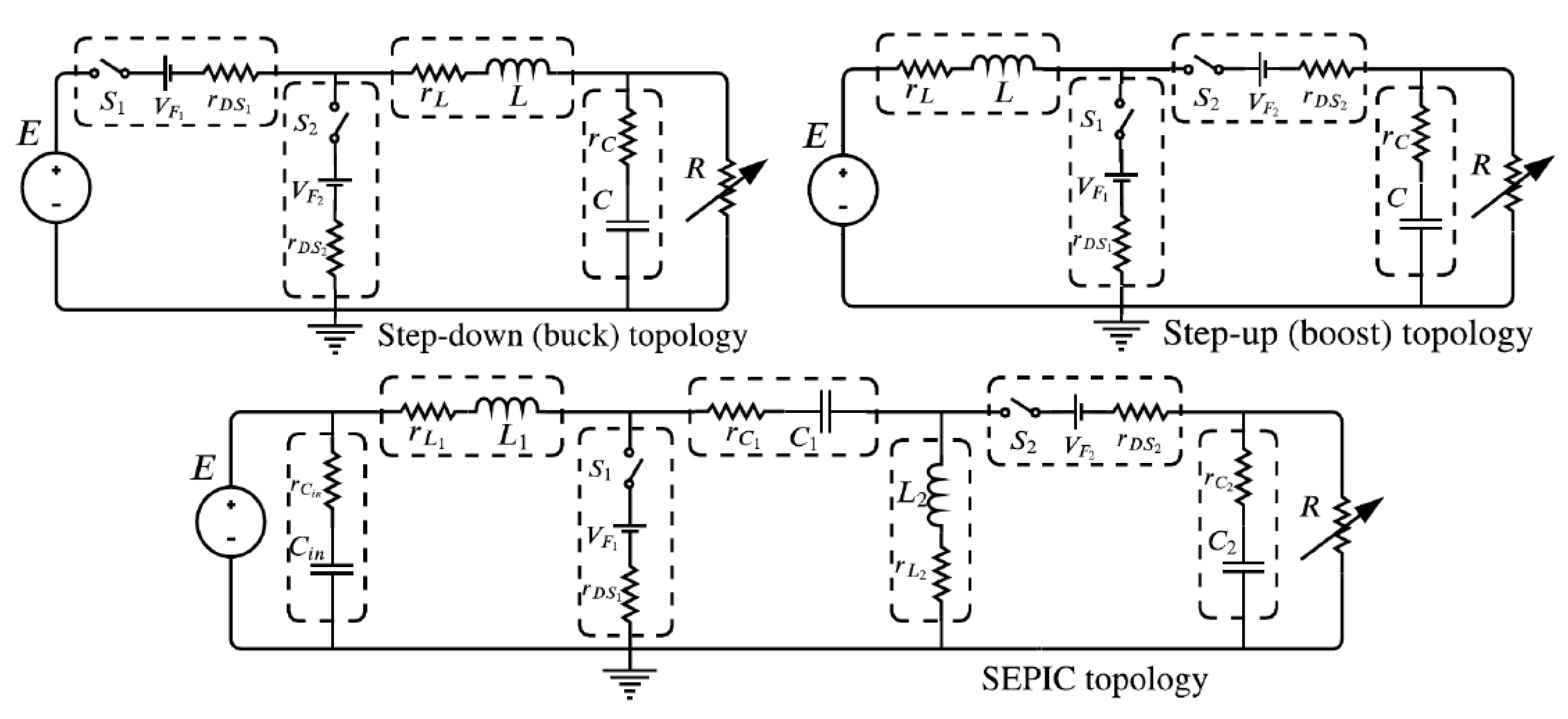
In this section we present detailed design and analysis steps of the proposed method and toolbox workflow only for the single-ended primary-inductor converter (SEPIC), for brevity. The nominal values of the SEPIC converter parameters used for this set of numerical simulations are presented in

Table 1. SEPIC topology parameters, values, along with corresponding tolerances.

Param.	Val.	Tol.	Param.	Val.	Tol.
$L_1$	$2.57$ [mH]	$\pm 20\%$	$L_2$	1.71 [mH]	$\pm 20\%$
$r_{L_1}$	130 [m$\Omega$]	$\pm 10\%$	$r_{L_2}$	110 [m$\Omega$]	$\pm 10\%$
$r_{D{S}_1}$	$0.01$ [$\Omega$]	$\pm 10\%$	$r_{D{S}_2}$	80 [m$\Omega$]	$\pm 10\%$
$C_1$	$4.7$ [$\mathsf{\mu }$F]	$\pm 20\%$	$C_2$	$3.57$ [$\mathsf{\mu }$F]	$\pm 20\%$
$r_{C_1}$	270 [m$\Omega$]	$\pm 10\%$	$r_{C_2}$	350 [m$\Omega$]	$\pm 10\%$
$C_{in}$	$3.57$ [$\mathsf{\mu }$F]	$\pm 20\%$	$r_{C_{in}}$	270 [m$\Omega$]	$\pm 10\%$
$V_{F_1}$	$0.2$ [V]	$\pm 10\%$	$V_{F_2}$	$0.62$ [V]	$\pm 10\%$

, along with their tolerances.

Firstly, we proceed to obtain the robust controller used for path planning, using the methodology presented in [14]. As such, we need to linearize the quasi-linear input-affine nonlinear system (${\Sigma }_{sepic}$) from Equation (57) according to Equation (30). This high-power configuration of the converter is targeted for renewable energy sources, with the desired input/state/output operating specifications being: output voltage $y_0\left(t\right)=u_R\left(t\right)=400$ [V], with a nominal external voltage source $E_0=300$ [V] and load input resistance $R_0=80[\Omega ]$. An initial guess for the state vector equilibrium point values was ${\tilde{\mathbf{x}}}_0=[300,10,300,-10,400]$, followed by ${\tilde{\mu }}_0=0.55$ for the duty cycle command. Through numeric computation, the nominal nonlinear plant equilibrium point follows:

$$\left({\mathbf{u}}_0,{\mathbf{x}}_0,{\mathbf{y}}_0\right)=\left(\left[300,80,0.5788\right],\left[300,6.8711,297.722,-5,400\right],400\right).$$

(64)

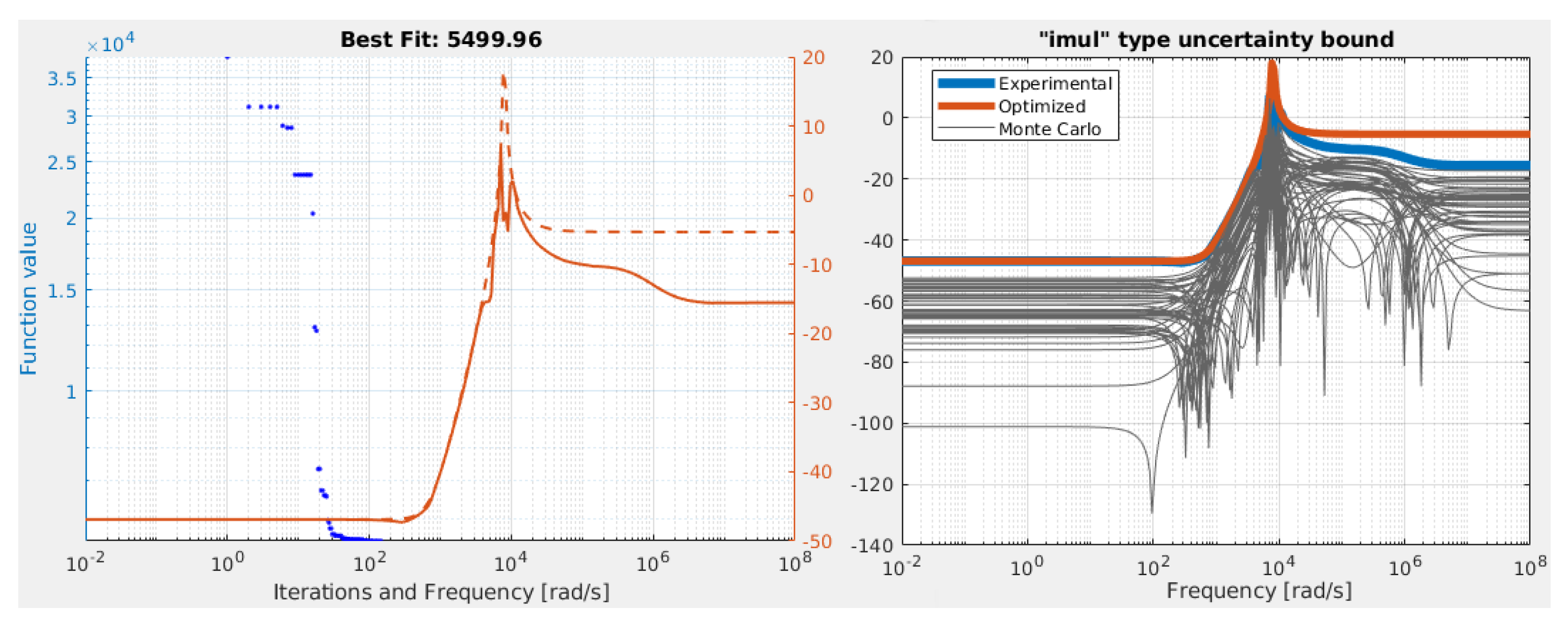
After calling the System.linearize() routine for the LTI plant model, the uncertainty model needs to be computed. For modelling the uncertainty of the electrical components and external influences, an input multiplicative model was considered, i.e., $G\left(s\right)=G_n\left(s\right)\left[1+\Delta \left(s\right)W_{unc}\left(s\right)\right]$, with ${\left|\right|\Delta \left|\right|}_{\infty }\le 1$. This model has been numerically computed in an automatic manner from the interface of input $u_3\left(t\right)\equiv \mu \left(t\right)$ to output $y_1\left(t\right)\equiv u_R\left(t\right)$, with the additional tolerances $E\in \left[290,310\right]$ [V] and $R\in \left[75,85\right]$ $[\Omega ]$, based on $N=1000$ Monte Carlo simulations. A comprehensive frequency range for this SEPIC configuration is $\left[\underline{\omega }={10}^{-2},\overline{\omega }={10}^8\right]$, with 300 equally distributed samples in logarithmic domain. For the particle swarm optimization algorithm used for computing the uncertainty bounds, a successful set of hyperparameters consists in the swarm size of 1500, initial swarm span of ${10}^3$, minimum neighbors fraction of $0.85$, and inertia range of $\left[0.15,1.15\right]$, for a complex pole and zero pair transfer function, resulting in:

$$W_{unc}\left(s\right)=K\frac{s^2+2{\zeta }_z{\omega }_{n_z}s+{\omega }_{n_z}^2}{s^2+2{\zeta }_p{\omega }_{n_p}s+{\omega }_{n_p}^2}=0.53201·\frac{s^2+1289s+4.623\mathrm{e}+5}{s^2+158.6s+6.286\mathrm{e}+7}.$$

(65)

This procedure and its validation is portrayed in Figure 7.

In minimal form, the linearized SEPIC plant family is spanned by fourth-order stable and proper systems, with four zeros, three of which are of nonminimum phase, from the control path to the load resistor voltage output. The nominal MISO transfer matrix model from $\mathbf{u}\left(t\right)\equiv {\left[\Delta R\left(t\right),\Delta E\left(t\right),\Delta \mu \left(t\right)\right]}^T$ to $y\left(t\right)\equiv \Delta u_R\left(t\right)$ is:

$${\mathbf{G}}_n\left(s\right)=\frac{s+8.003\mathrm{e}+5}{\alpha \left(s\right)}\left[\begin{array}{c}5.925\mathrm{e}+7(s^2+162.5s+7.202\mathrm{e}+7)\\ 0.021779(s+346.5)(s^2+179.7s+5.637\mathrm{e}+7)\\ 4.1368(-s+2.304\mathrm{e}+4)(s^2-717.4s+5.145\mathrm{e}+7)\end{array}\right],$$

(66)

where $\alpha \left(s\right)=(s^2+2673s+3.749\mathrm{e}+7)(s^2+1339s+6.493\mathrm{e}+7)$.

Besides the classical scope of obtaining good transient and steady-state responses, another main purpose for the controller synthesis was to penalize near-resonance control effort, as the obtained controllers would otherwise be difficult to implement in practice, requiring small sampling periods, i.e., $T_s<50$ [$\mathsf{\mu }$s]. As such, the sensitivity, complementary sensitivity and control effort loop-shaping filters are:

$$W_S\left(s\right)=\frac{0.5s+200}{s+2},W_T\left(s\right)=\frac{s^2+4000s+4\mathrm{e}+6}{1\mathrm{e}-4s^2+56.57s+8\mathrm{e}+6},W_{KS}\left(s\right)=\frac{100s+346.5}{s+346.5},$$

(67)

with an imposed sensitivity bandwidth of at least ${\omega }_B$= 200 [rad/s], admissible steady-state error of maximum $A={10}^{-2}$, allowed sensitivity peak at $M=2$. Lower bandwidth was imposed for damping the frequency response resonance and, also, to move away from the physical limitations of the multiple nonminimum phase zeros. The complementary sensitivity bandwidth must be faster than ${\omega }_{BT}=2000$ [rad/s], forcing a high frequency attenuation of at least $A_T={10}^{-4}$ with a roll-off order $n=2$, with an allowed peak of $M_T=2$. The dynamic control effort weighting function imposes all frequencies with magnitude less than 1, with a further penalization of maximum $0.1$ above $\omega \approx 1000$ [rad/s], due to the resonant peak centered at $\omega \approx 9000$ [rad/s].

From the direct application of the $\mu$-synthesis procedure for the augmented plant with uncertainties, a controller of order $n=19$ is obtained. This procedure is followed by a balanced order reduction operation, with the smallest-order controller which manages to ensure all imposed performance specifications, with a peak value ${\mu }_{\Delta }\left(\mathtt{LLFT}(P,K)\right)\le 0.901513<1$, being of order $n=3$:

$$K_{rob}^{SEPIC}=\left(\begin{array}{cccc}-1.997& 3.257& -3.706& 0.5324\\ -3.257& -2294& 6474& 0.434\\ -3.702& -6474& -1.539\mathrm{e}+04& 0.4941\\ ine0.5324& -0.434& 0.4941& 0\end{array}\right).$$

(68)

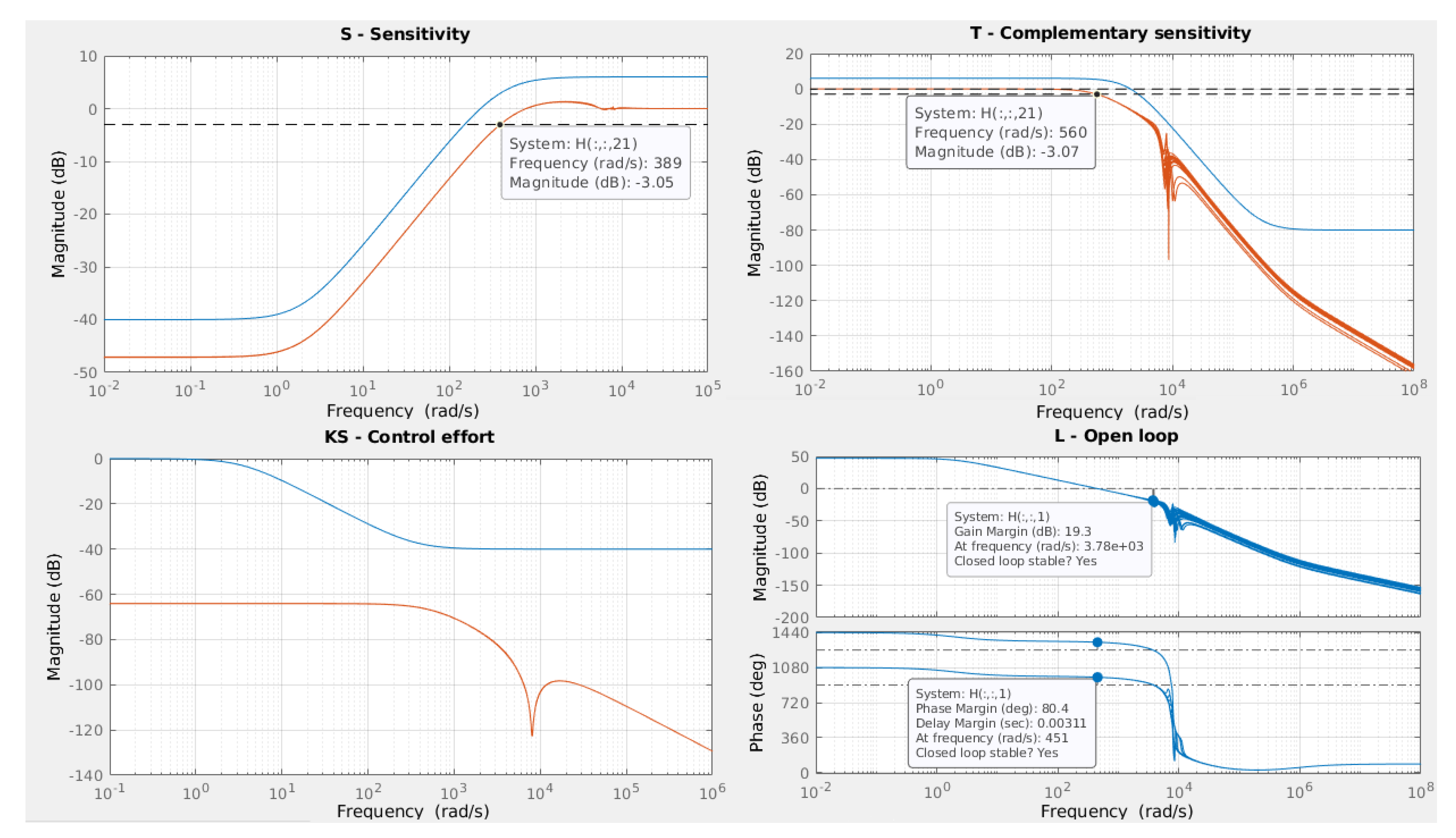
The robust path-planning design of the weighting filters, along with frequency response closed-loop performance plots with the reduced-order controller for the uncertain SEPIC converter plant set are illustrated in Figure 8 and Figure 9. The closed-loop control system presents itself with large stability margins, with a phase margin ${\gamma }_k\approx 80{[}^{\circ }]$ and gain margin of $m_k^{dB}\approx$ 19 [dB]. Additionally, as specified by the parameters $n=2$ and $A_T={10}^{-4}$ of $W_T\left(s\right)$, the closed-loop control system practically nullifies stochastic sensor noise signals spanning from ${\omega }_{BT}>2000$ [rad/s], using an initial roll-off of $-40$ [dB/dec], followed by an attenuation of at least four orders of magnitude. In practice, the attenuation continues with a further $-20$ [dB/dec] roll-off afterwards.

From the frequency response of Figure 8, the bandwidth is measured at ${\omega }_B\approx 390$ [rad/s], resulting in an equivalent rise time less than $t_r\approx$ 2.5 [ms], with a negligible steady-state error ${\epsilon }_{ss}\approx$10${}^{-2}\times (y_{ss}-y_0)=0.2$ [V], where $y_{ss}$ represents the steady-state value, relative to the desired equilibrium output $y_0=400$ [V]. Additionally, the system presents no overshoot in the vicinity of the operating point, as it was designed to behave similar to a first-order low-pass filter.

The SEPIC converter is a highly-nonlinear plant with respect to the command signal $\mu \left(t\right)$, and there are use cases where the operating point may be dynamic, along with being generally affected by a diverse set of perturbations. Besides the previously-mentioned advantages of the already designed robust controller, it will be used as an auxiliary path planning component along with the K-PBC controller used to guarantee asymptotic stability for the entire domain of operation for the converter.

In order to design the K-PBC controller, we need to construct the output port-variable $h_K(\mathbf{x},\mathbf{u})$ such that the SEPIC converter is Krasovskii passive. The LMI problem presented in Claim 3, having the bounds of the load resistance $R\in [10,1000][\Omega ]$, has been solved using the method described in [13], with a possible solution from the feasibility cone:

$$Q=1\mathrm{e}-03·\left[\begin{array}{ccccc}0.000714& 0& 0& 0& 0\\ 0& 0.514& 0& 0& 0\\ 0& 0& 0.00094& 0& 0\\ 0& 0& 0& 0.342& 0\\ 0& 0& 0& 0& 0.000714\end{array}\right],$$

(69)

from which the output port-variable have the form presented in Claim 3, as well.

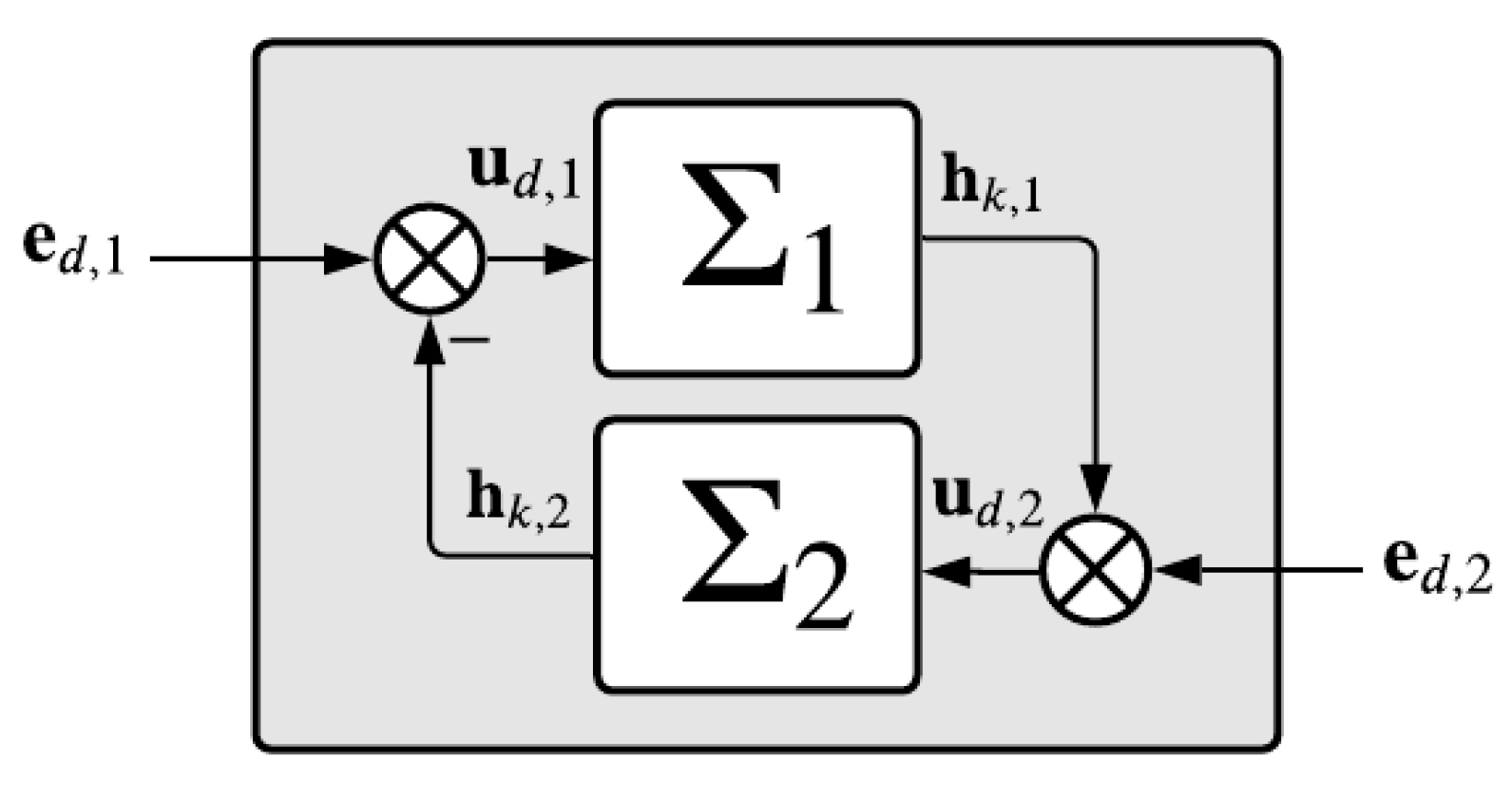
After this extra output is designed, the K-PBC having the form:

$$\left({\Sigma }_{K-PBC}\right):\left\{\begin{array}{c}{\dot{\mathbf{x}}}_c=K_1(K_2({\mathbf{x}}_c-{\mu }^{🟉})-h_K\left(\mathbf{x}\right))\hfill \\ {\mathbf{y}}_c={\mathbf{x}}_c\hfill \end{array}\right.,$$

(70)

having two inputs: the output port-variable $h_K\left(\mathbf{x}\right)$ of the extended $\left({\Sigma }_{\mathrm{sepic}}\right)$ and the desired input trajectory ${\mu }^{🟉}$, while the output is the actual value of the duty-cycle $\mu \left(t\right)\equiv y_c\left(t\right)$. The parameters of the controller (Equation (70)) are $K_1=3\times {10}^{-5}$ and $K_2={10}^8$.

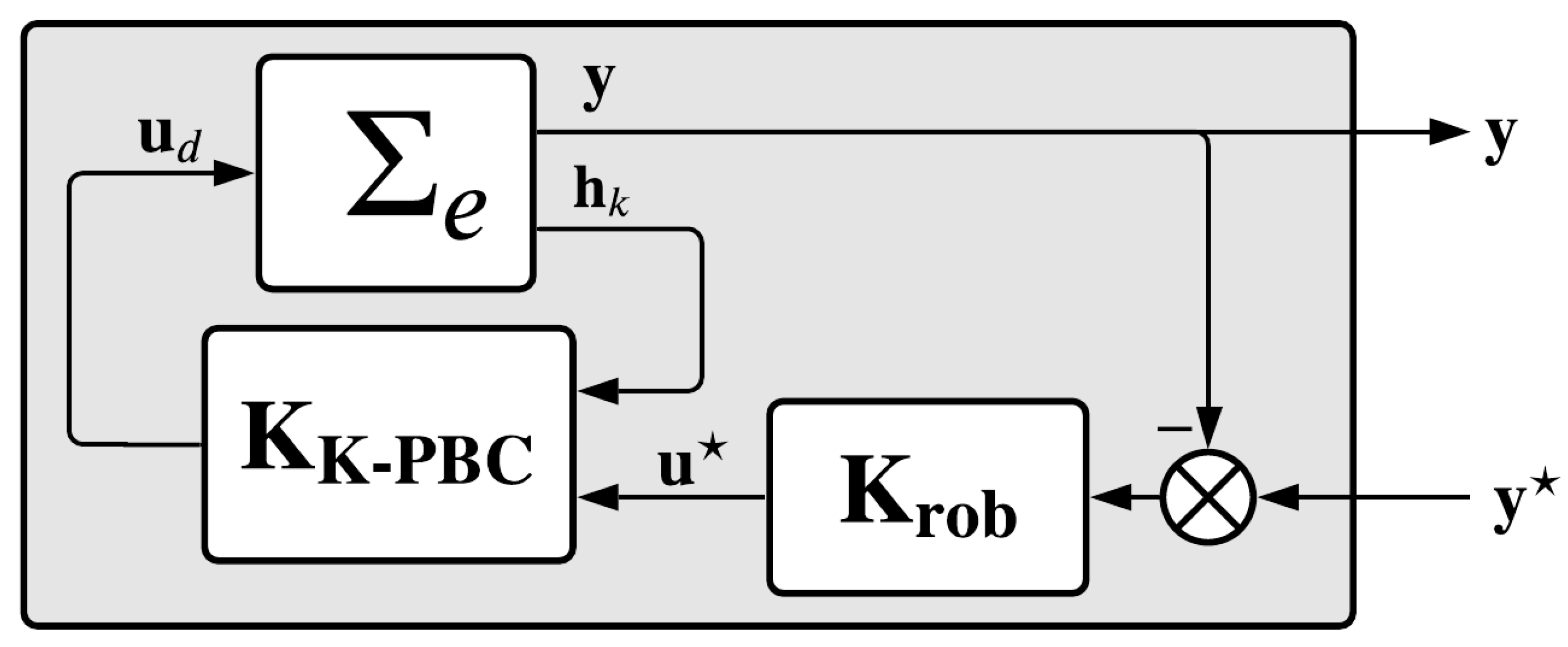
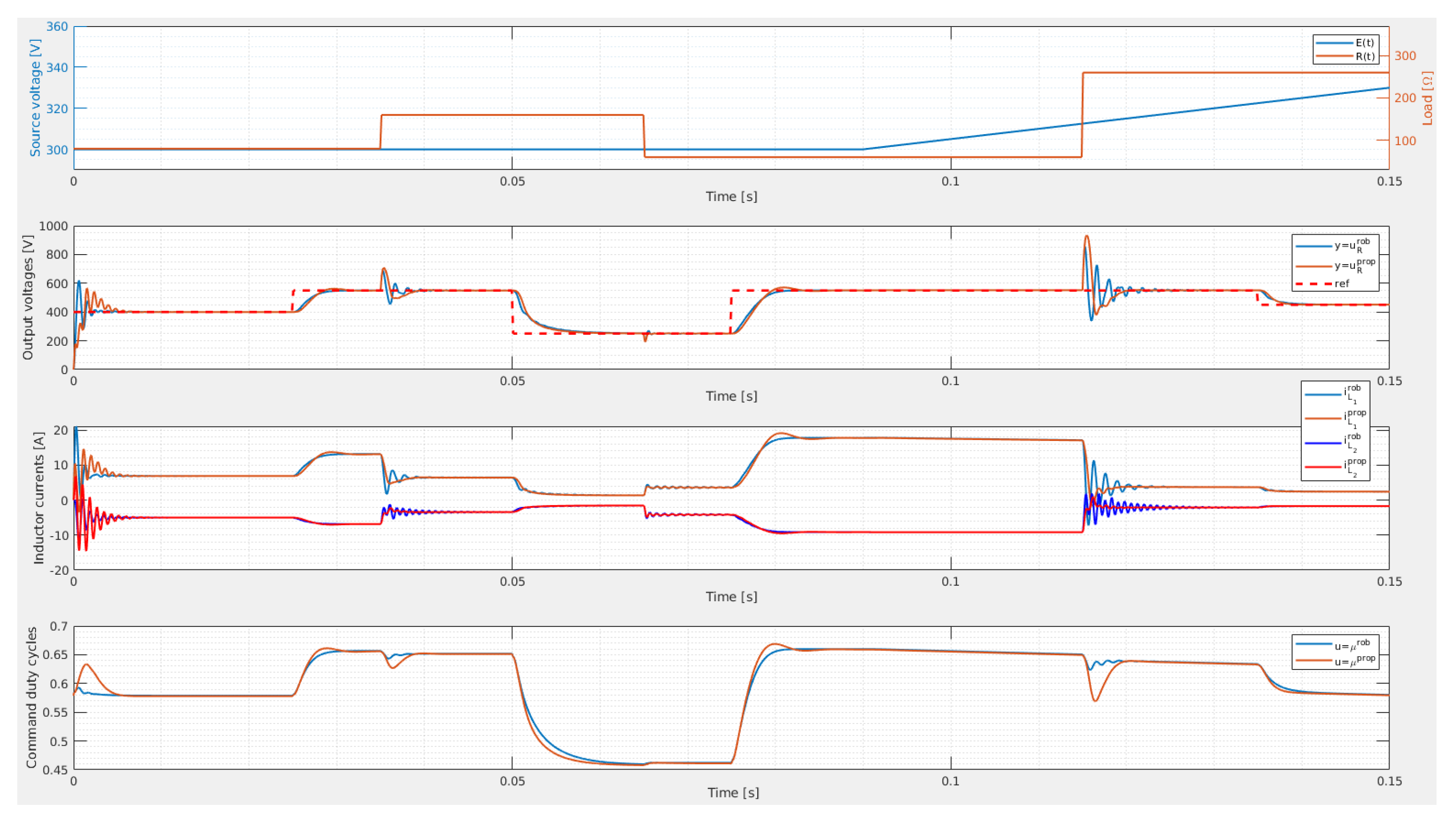
Figure 9 and Figure 10 illustrate time domain simulations of the SEPIC converter in closed-loop configuration using the proposed control structure of cascaded K-PBC with $\mu$-synthesis path planning ${\mathbf{K}}_{rob}$ at various operating points, as in Figure 3, along with different types of disturbances applied, in comparison to using the same robust controller-only approach, using the structure from Figure 4. The former compares the response of the proposed closed-loop system by comparison with the robust controller only counterpart, while the latter figure illustrates the robust stability and robust performance of the proposed method for a set of 50 Monte Carlo simulations sampled from the tolerance set of Table 1.

Both experiments start from null initial conditions applied to all state variables, in order to emphasize the behaviour to sudden jumps in the dynamics, followed by a succession of disturbances applied at the converter inputs, such as:

• a sequence of load resistance steps:

  -

  from $R(t_1^{-}=0.035-)=80$ [$\Omega$] to $R(t_1^{+}=0.035+)=160$ [$\Omega$];

  -

  from $R(t_2^{-}=0.065+)=160$ [$\Omega$] to $R(t_2^{+}=0.065+)=60$ [$\Omega$];

  -

  from $R(t_3^{-}=0.115+)=60$ [$\Omega$] to $R(t_3^{+}=0.115+)=260$ [$\Omega$].

• a ramp disturbance on the external source voltage from $E(t<0.090)\equiv 300$ [V], starting at $t_4=0.090$ [s] with an increasing slope of 500 and saturated at 50 [V];
• a sequence of output reference steps:

  -

  from $u_R^{*}(t_5^{-}=0.025-)=400$ [V] to $u_R^{*}(t_5^{+}=0.025+)=550$ [V];

  -

  from $u_R^{*}(t_6^{-}=0.050-)=550$ [V] to $u_R^{*}(t_6^{+}=0.050+)=250$ [V];

  -

  from $u_R^{*}(t_7^{-}=0.075-)=250$ [V] to $u_R^{*}(t_7^{+}=0.075+)=550$ [V];

  -

  from $u_R^{*}(t_8^{-}=0.135-)=550$ [V] to $u_R^{*}(t_8^{+}=0.135+)=450$ [V].

As noticeable in Figure 9, the proposed method not only tracks the desired voltage reference at all operating points, but it also considerably improves transients caused by changes in the disturbance signals compared to using ${\mathbf{K}}_{rob}$ only, such as for the moments t = 0, $t_1$, $t_2$, $t_3$, with smaller overshoots and more damped oscillations. A small compromise is that it adds insignificant overshoots when reference changes occur, such as at time $t_6$. The steady-state performance is not affected by the addition of the K-PBC.

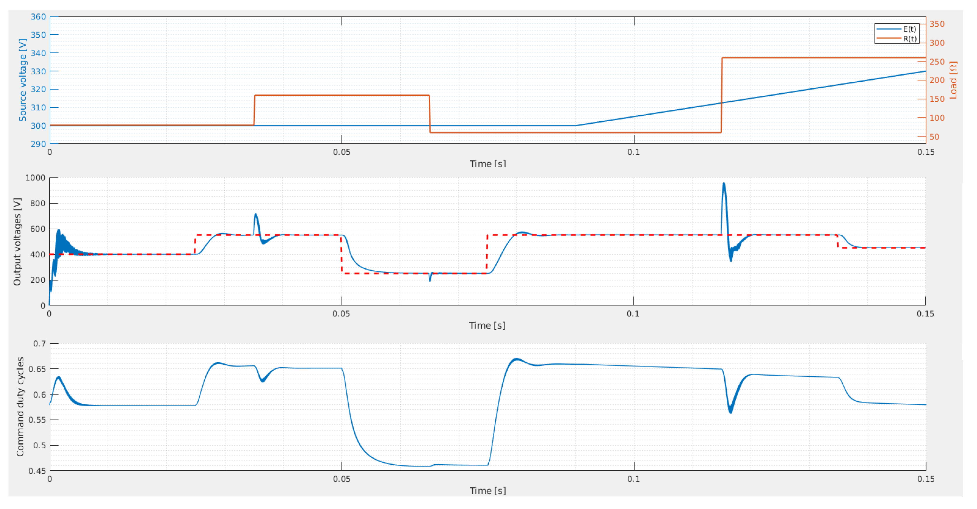
In addition to the previous results, Figure 10 shows the robustness of the method when subjected to the parametric uncertainties inherent to the SEPIC converter circuit, in which all the dynamic and steady-state performance indicators remain fundamentally unchanged even after $\pm 20\%$ variations of the circuit’s main component values.

6. Conclusions

The current paper presents a mathematical framework which allows to construct an output vector such that an input-affine nonlinear system is Krasovskii passive. Moreover, Theorem 3, which is a convex particularization of Theorem 1, without any dependency on the state variable $\mathbf{x}$, provides the set of necessary and sufficient conditions for a quasi-linear affine system to be Krasovskii passive in terms of LMIs. To illustrate the flexibility and usefulness of the method, as a case study, a unified treatment for DC-DC converters is presented. After this interface is set for such a system, a method to construct a K-PBC is presented. The LLFT interconnection between the nonlinear system and K-PBC ensures the asymptotic stability, which means that the closed-loop system manages to follow the given input trajectory. However, the input trajectory has the same physical significance as the input of the nonlinear system, which, in general, differs from that of the output. As such, another component, called path planner, is mandatory in order to obtained the desired tracking performance. The proposed method includes a dynamical path planning as a robust controller computed for the linearized plant around the desired equilibrium point by solving the mixed-sensitivity $\mu$-synthesis loop-shaping problem. In brief, the decentralized controller manages to ensure the asymptotic stability due to the K-PBC component, while the robust controller manages to compute the input trajectory such that the closed-loop system fulfills the robust performance.

Although Section 4 presents the possibility to compute the output port-variable such that various DC-DC converter topologies are Krasovskii passive, in Section 5 we present the SEPIC converter as a case study, due to its highly-nonlinear behaviour. As shown in the previous section, there are some important improvements if we compare the results obtained with the proposed method against the results obtained with the robust controller only. Moreover, the robustness of the proposed method has been proved using Monte Carlo simulations in time domain.

In this paper we managed to develop the mathematical background, which was successfully implemented in a second version of our toolbox, initially presented in [14]. However, in this current iteration we assume that all signals required for the output port-variable construction are available. But, in practice, an estimator will be necessary. As such, one possible extension for practical implementation could consist in (1) considering a high-gain observer for quasi-linear affine systems. Additionally, (2) there are three degrees of freedom for the K-PBC controller—the matrices Q, $K_1$ and $K_2$—which may also be introduced in the optimization problem when computing the robust controller. Finally, (3) the implementation of the proposed method on microcontroller units will be studied, by also taking into consideration quantization effects.