1. Introduction
In 2017, the aviation sector contributed approximately 5% of the global anthropogenic RF, with the RF attributed to contrails and contrail cirrus being estimated as 50 mW/m
2, making it the largest contribution in the sector [
1]. Yet, contrail cirrus have a much shorter lifetime than long-lived greenhouse gases, which influences their relative importance when it comes to estimating the long-term climatic impact of the aviation sector [
2], and also makes them very suitable for mitigation efforts as the effects would become very quickly apparent [
3].
It is generally agreed that the RF of contrail cirrus will increase in the coming years. This increase was estimated to occur by a factor of 3 from 2006 to 2050, reaching 160 or even 180 mW/m
2 by that year, attributed to both a large increase in air traffic and a slight shift in the air traffic towards high altitudes [
3,
4].
There was indeed a continuous increase in commercial air traffic up to the year 2019, but a steep decrease in 2020 ended this trend [
5], due to the global COVID-19 pandemic. While it is uncertain when the aviation sector will recover, this decline in air traffic is not considered to be everlasting or to mark an end to the aviation industry. As of now, central traffic forecasts used for 2050 predictions have decreased 16% compared to 2019 forecasts for the same year [
6], which greatly impacts past predictions. Nevertheless, without the implementation of mitigation measures, it appears that this will result in a simple breather rather than a fix to the present problem.
Whereas cirrus clouds require high ice supersaturation to form, contrail cirrus can form when the environment is just at ice saturation, yet their conditions for evaporation are the same as those for cirrus clouds. This means that in a substantial fraction of the upper troposphere, contrail cirrus can form and persist in air that is cloud-free, increasing the high cloud coverage in environments where cirrus clouds would not be able to form.
The alteration of flight paths to avoid the ice-saturated and low-temperature regions where contrails typically form has been previously considered as a contrail mitigation measure [
7,
8]. This strategy could potentially go one step further; contrails have far greater regional effects than those expected from global mean values, which could potentially aid mitigation efforts by avoiding flights in regions where contrails warm the Earth and increasing them in regions where contrails cool it [
9]. Yet, this strategy could result in significant increases in both flight time and cost [
8]. Additionally, while some estimates place the contribution of contrail cirrus to the aviation sector RF far above all remaining contributions, other estimates place it only slightly above CO
2 emissions. In this case, the increased CO
2 emissions could overtake any benefits gained through the decrease in contrail emissions [
2].
There have also been numerous design-based strategies to mitigate contrails, but they tend to share one characteristic: the need to overhaul current aircraft in lieu of the more climate-friendly designs [
10]. While further research could reveal these to be good long-term solutions, interim solutions which can use the current infrastructure would still be needed; the subject of this work is one such solution.
This work focuses on the reduction of soot particles as a strategy to mitigate the climatic impact of contrails. A reduction of up to one order of magnitude in soot particle emissions, from the typical range of
–
soot particles/kg-fuel, is expected to lead to approximately the same reduction in the number of ice particles in the formed contrail [
11,
12]. Experiments conducted as early as 1984 found that decreases in a fuel’s aromatic content lead to a substantially reduction in soot emissions due to its combustion [
13]. SAF, which tend to have a much lower aromatics content, have thus long been expected to yield lower soot emissions, but also higher water vapour emissions that could contribute to an increase in the frequency of contrail formation.
A few years ago, a report [
1] was published presenting the data obtained in several test flights which used a 50:50 blend of low-sulfur Jet A fuel and a HEFA C. biojet fuel. During the test flights, it was found that soot particle emissions could be up to over 50% lower for the HEFA C. blend when compared to a Jet A fuel with medium sulfur content, which was associated to a reduction in ice mass content in contrails.
In 2018, global simulations [
14] were carried out to ascertain the impact on the radiative forcing of contrails for a global decrease of 80% and 50% in soot emissions compared to current conventional jet emissions, such as could be found when using alternative fuels or lean combustion. These led to reductions in radiative forcing of 50% and 20%, respectively. Later, additional simulations [
3] were run for the year 2050, which took into account an increase in air traffic, changes in the background climate, an increase in propulsive efficiency, a 50% reduction in soot emissions, and a further 15% decrease in water emissions; the reduction in soot emissions led to a decrease of 15% in the radiative forcing of contrails when compared to simulations considering typical emissions from conventional aviation fuel.
The present study seeks to further investigate the influence of SAF on contrail formation and contrail cirrus properties, taking into account the effect of the differences in soot emissions, water vapor emissions, and other combustion and exhaust properties. It goes into detail about the influence of these properties on the different stages of a contrail’s lifetime, taking into account both the environment of formation and the fuel burned.
2. Modeling Approach
As the purpose of this work is to study the impact of SAF on contrail and contrail cirrus, an engine model capable of distinguishing between fuels during combustion is required. To this effect, a 0-D engine model by Gaspar and Sousa [
15] was implemented. This model takes as inputs the TAS of the aircraft, the flight altitude, the fuel to be simulated, and the blend ratio.
The engine model [
15] was conceived with the goal of studying the engine performance and pollutant emissions when burning SAF instead of conventional aviation fuels; this makes it ideal for this implementation. The model is extensively documented and validated in the literature, and only suffered minor alterations with the objective of reducing its computation time for this work. It was originally designed to run once per program run, while in this work it runs once per route point; this vastly increased its run time, and brought to light some critical computational bottlenecks. Resolving these issues did not alter the results or the modeling of the engine.
This study simulated the combustion of pure SAF and of SAF blended with a Jet A-1 fuel. The properties of the simulated fuels and the model for the estimation of the blend properties were obtained from the study by Gaspar and Sousa [
15], and the former are summarized in
Appendix A.
The blends were simulated at a 50:50 blend ratio, with the exception of the SIP blend which was considered with 10% SIP content only; these are the currently certified maximum blend ratios for the simulated SAF. As of now, the use of pure SAF is not certified for commercial flights. When SAF are burnt alone, their lack of aromatic content hinders the swelling of the nitrile O-rings which are typically used by the aviation sector; this can lead to fuel leakage, and is thus of great concern. Current regulations require a minimum of 8% aromatic content in a fuel blend to prevent this. However, newer O-rings fabricated from fluorocarbons do not require the swelling effect of aromatics. This could eventually lift the minimum aromatic content regulations if it was proven to no longer be necessary, making future flights with pure SAF a possibility [
16]; taking this possibility into account, simulations for pure SAF were also run and are presented here.
The engine model [
15] was coupled with the Rizk and Mongia model [
17] for the prediction of the soot emissions by the different fuels. The Rizk and Mongia model [
17] is an empirical model used for the calculation of soot mass emissions which takes into account the soot formation and the soot oxidation. In this work, soot mass emissions obtained with this model are converted into particle emissions using a mean radius for the primary particles, which are assumed to be spherical. A mean particle volume is computed from this radius and used, along with the soot density (
kg/m
3), to relate the soot mass with the soot particle number.
The current understanding of soot formation dynamics establishes that particle number variation is not proportional to particle mass variation; soot particle radius increases with engine power, and shows marked differences depending on the fuel used. In particular, SAF blends with lower aromatics than typical Jet A-1 fuel have been shown to produce soot particles with a smaller mean radius [
18].
Unfortunately, not enough data are available to establish a correlation between a fuel’s composition, engine power, and the aggregate and primary particle sizes ensuing from the combustion, thus a mean radius is established for all fuels based on typical Jet A emissions for modern aircraft [
19]. This could potentially lead to an underestimation of SAF soot particle emissions.
The life and properties of the contrails are simulated with a model based on the CoCiP model developed by Schumann [
20]. This modeling approach requires several local atmospheric parameters as inputs, which were obtained from the ERA-20CM model ensemble for the year 2010 [
21]. The parameters obtained from this model were the northward and eastward winds, the pressure change rate, the ambient temperature, and the ambient relative humidity. The ensemble gives the mean monthly values for a set of local atmospheric parameters at different latitudes, longitudes and pressure levels; this allows the atmosphere to be modeled in three-dimensional space.
Contrails are formed when the SAC is satisfied, that is, when the ambient temperature is below a critical temperature which is a function of the water vapor emissions, the net heat of combustion, and the propulsive efficiency, as well as the ambient temperature, absolute humidity, and pressure. The latter are gathered from the ERA-20CM data, while the former are obtained from the tabulated fuel properties and engine model outputs. The engine in the model is a two-spool turbofan of the same type as the Lycoming ALF 502 engine, and the aircraft dimensions were correspondingly modeled after the BAe 146.
The wake vortex phase immediately after contrail formation is not resolved; instead, contrail properties at the end of this phase are estimated using a parametric model. The parametric model is formulated in normalized form, with the characteristic scales based on initial vortex separation
and circulation
; this leads to the timescale
, represented in Equation (
3). The initial vortex separation is proportional to the aircraft wingspan
, and the circulation is a function of the ratio of the aircraft weight
to the product of the aircraft wingspan by the air speed and density.
The EDR, denoted here by symbol
, is normalized using the initial vortex separation and the initial descent speed
; in turn, the Brunt–Väisälä frequency
is normalized using the timescale
.
To simulate the contrail ice properties at the different stages of its life, two plume bulk ice quantities are used: the mass mixing ratio of ice in the contrail and the total number concentration of contrail ice particles per contrail length. The initial number of ice particles is set to be the number of soot particles that were emitted during combustion, which is consistent with previous model results [
11,
12].
The advection of the contrail is calculated using a second order Runge–Kutta scheme, with the latitude and longitude changing due to the northward and eastward winds. Additionally, the contrail is assumed to follow the mid-point of the bulk of ice particles under sedimentation, being displaced downward according to the ice particle terminal fall velocity
. The ice particle terminal fall velocity is found using Equation (
7), where
is the air dynamic viscosity,
denotes the air density,
is the maximum dimension of an ice crystal, and
stands for the Reynolds number [
22].
The maximum dimension of an ice crystal varies with temperature and crystal shape. In this work, it was estimated based on published measurements made on high-resolution images of ice crystals in cirrus clouds [
23].
The contrail dimensions, ice mass, ice particle number, and optical depth are calculated at each contrail trajectory point. A contrail’s lifetime is considered to end when its ice mass contents reaches zero, or when its optical depth reaches a small enough value, namely, . The CoCiP model also ended contrail simulations when the ice particle number concentration became too small, namely, particles/L. However, the latter criterion was not enforced in this work since the difference in ice particle number between fuels is one of the main topics of study.
2.1. Validation of Contrail Modeling
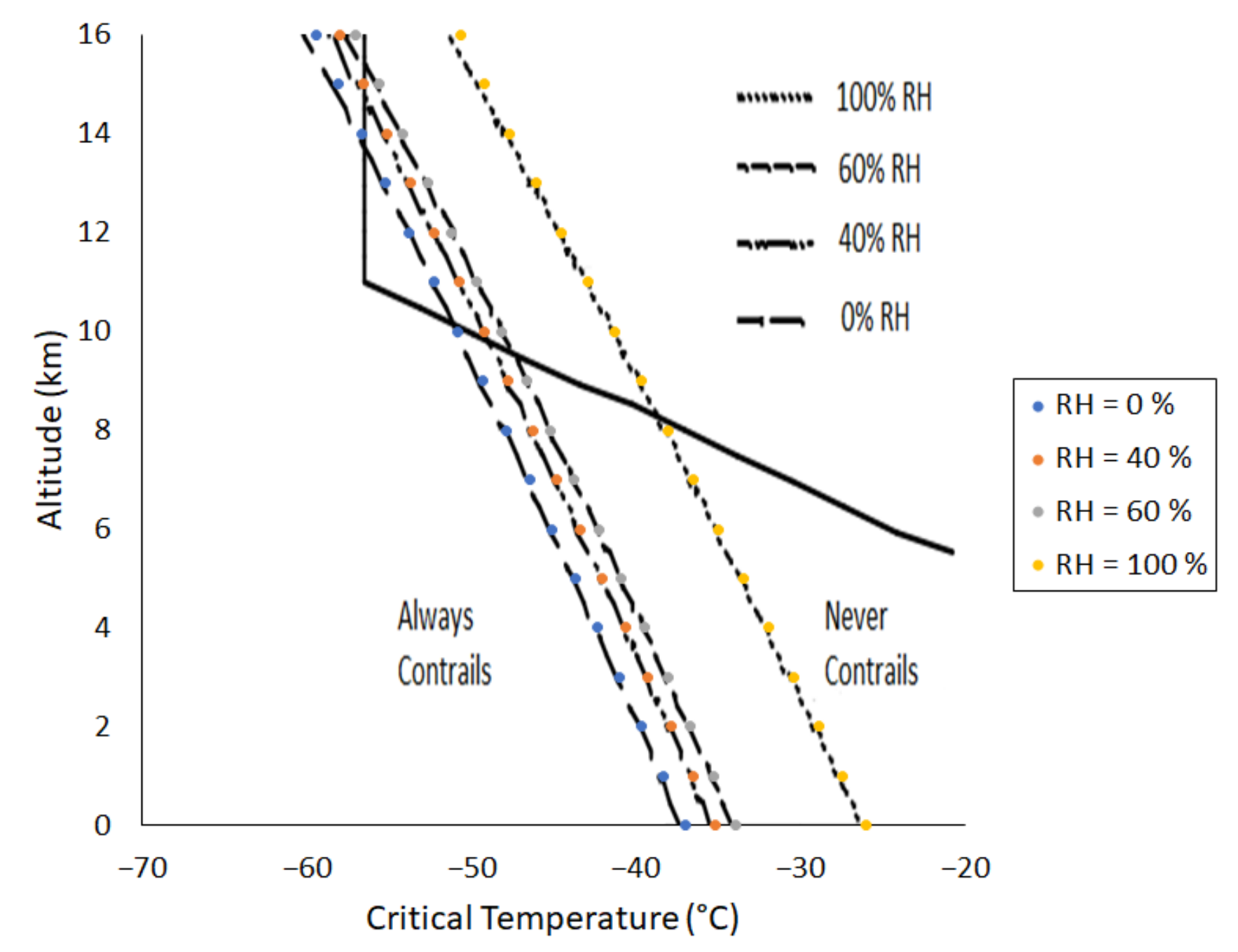
Figure 1 shows a comparison between the threshold temperatures obtained in this study using the SAC with those expected, for specified engine and fuel parameters. In this figure, the continuous thick line is the temperature profile of the standard ISA atmosphere.
Table 1 shows the comparison between the computed and measured values for the maximum displacement
, produced during the wake down vortex phase for an aircraft with dimensions equivalent to a A319-111, flying at
m/s on flight level
hft. This was one of the aircraft for which measurements were made in reference [
25], and it was chosen as its dimensions were the closest to what an aircraft with the engine modeled in this work would have. The table also shows the comparison between the ambient temperature
T, the Brunt–Väisälä frequency, and the normalized parameters computed with the model as well as obtained from the measurements.
The largest difference comes from the computed Brunt–Väisälä frequency, which shows an error of 35.29%. This can be shown to be responsible for the −19.41% error in the maximum displacement value; if the Brunt–Väisälä frequency is set to , the value obtained is m, with an error of only −0.05%. Nevertheless, a difference of 20 or even 30 m between the measured and computed values was expected and is still acceptable.
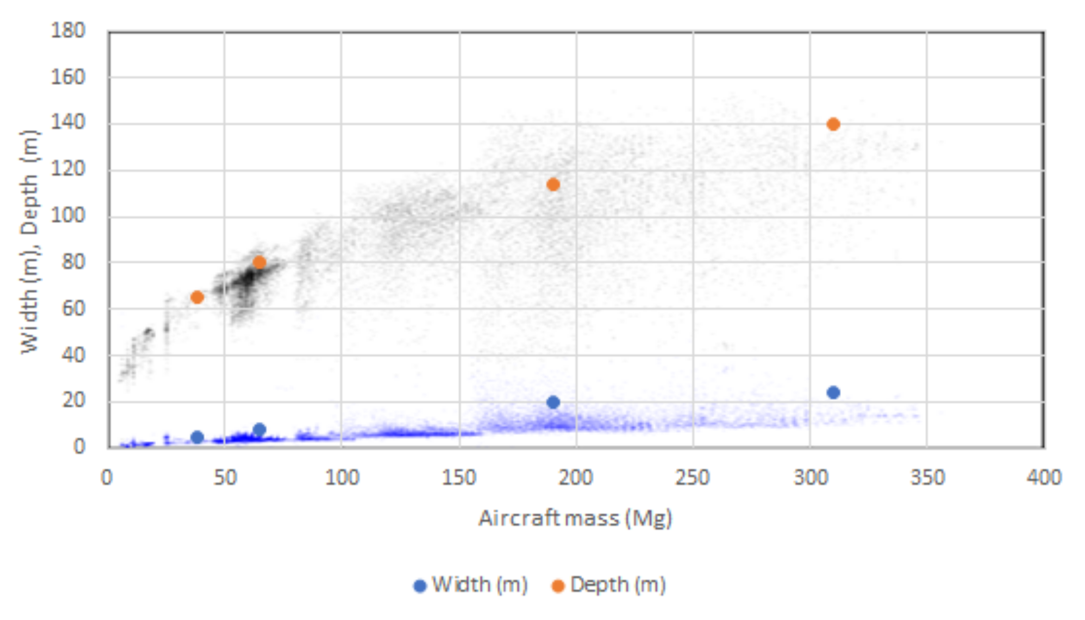
Figure 2 represents the predicted values for the initial contrail dimensions after contrail sinking due to the wake vortex downwash for different aircraft. The smallest example aircraft has the same dimensions as the BAe 146, the aircraft used for the simulations in this work, and the remaining aircraft are sample aircraft of the types B747, A330, and B737, with aircraft mass, wing span, flight speed, and fuel flow taken from in [
20]. The predicted values show an overall good agreement with the observed trend, the largest deviation from the mean occurring for the initial width of the sample large aircraft, with it nevertheless remaining within the expected scatter.
2.2. Validation of Particle Emissions Modeling
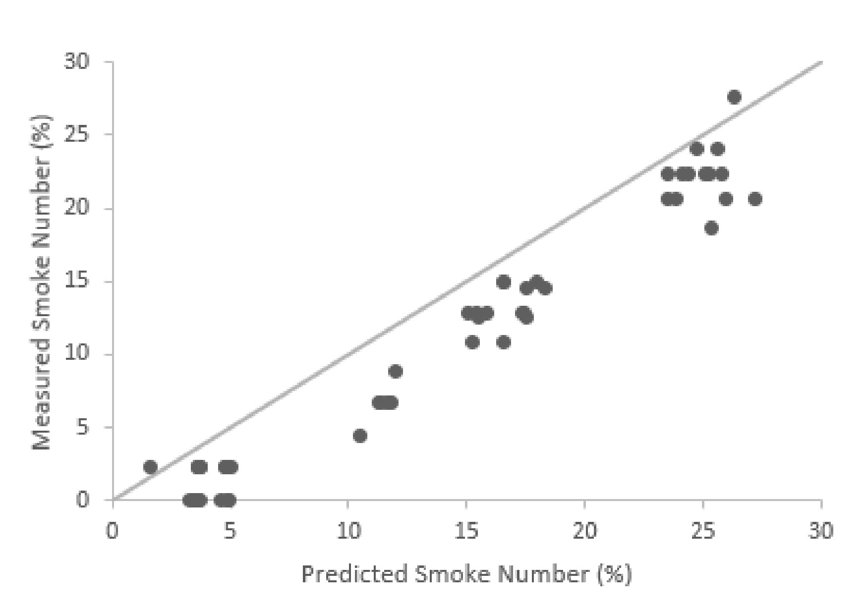
Figure 3 shows the correlation between the smoke number measured for the aero-engine Lycoming ALF 502 [
26] and the smoke number predicted with the Rizk and Mongia model [
17] for similar conditions. It can be concluded that this model tends to slightly overpredict the smoke number, but still showing a fairly reasonable correlation.
Table 2 compares the Relative Differences (RDs) in particle emissions obtained with the Rizk and Mongia model [
17] with those measured in flight tests; the comparison is done between a 50:50 blend of HEFA C. with a low-sulfur Jet A fuel, and a medium-sulfur Jet A fuel. The aircraft had four wing-mounted engines, with the exhaust plumes of the two inboard engines being measured; the data from both engines are presented, marked as Engine 1 and Engine 2.
The data are also presented with respect to different thrust settings of the engine (high, medium, and low). It can be seen that measured data showed smaller RDs for high thrust settings, and higher RDs for low thrust settings. In contrast, the model seems almost insensitive to this variation. The model accounts for variations in fuel flow, and the particle emissions vary significantly for the different thrust settings; it is the RDs between blend emissions and Jet A-1 emissions that show little variation. This lack of sensitivity could be attributed to the use of a mean radius which does not vary with thrust settings. As the simulations in the following section are all carried out for average medium-thrust cruise conditions, this should not be considered as a major shortcoming of the present modeling procedure, but it is still worthy of note.
3. Results and Discussion
The results obtained were heavily dependent on local environmental conditions, which often led to a very high dispersion in their values; to illustrate this, most results will be presented in “box and whisker” plots. A box-plot marker is constituted by a rectangular box which represents the interquartile range (with 50% of the results contained in it), split by a line which represents the median, and with two whiskers at its ends which extend up to 1.5 times the box length; this can be seen as a simplified representation of a density curve, with its peak corresponding to the median. Outliers are represented in these plots as isolated dots, and the mean value is further represented by a cross.
3.1. Contrail Formation Frequency
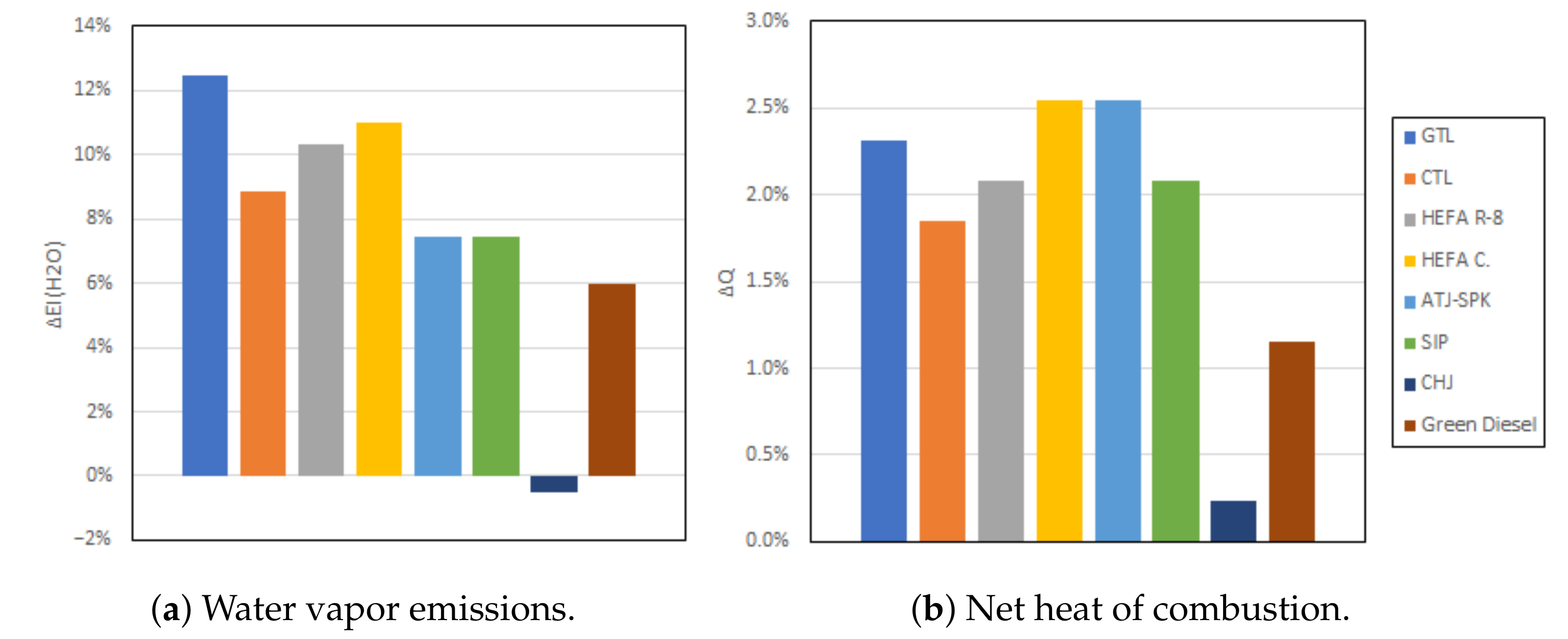
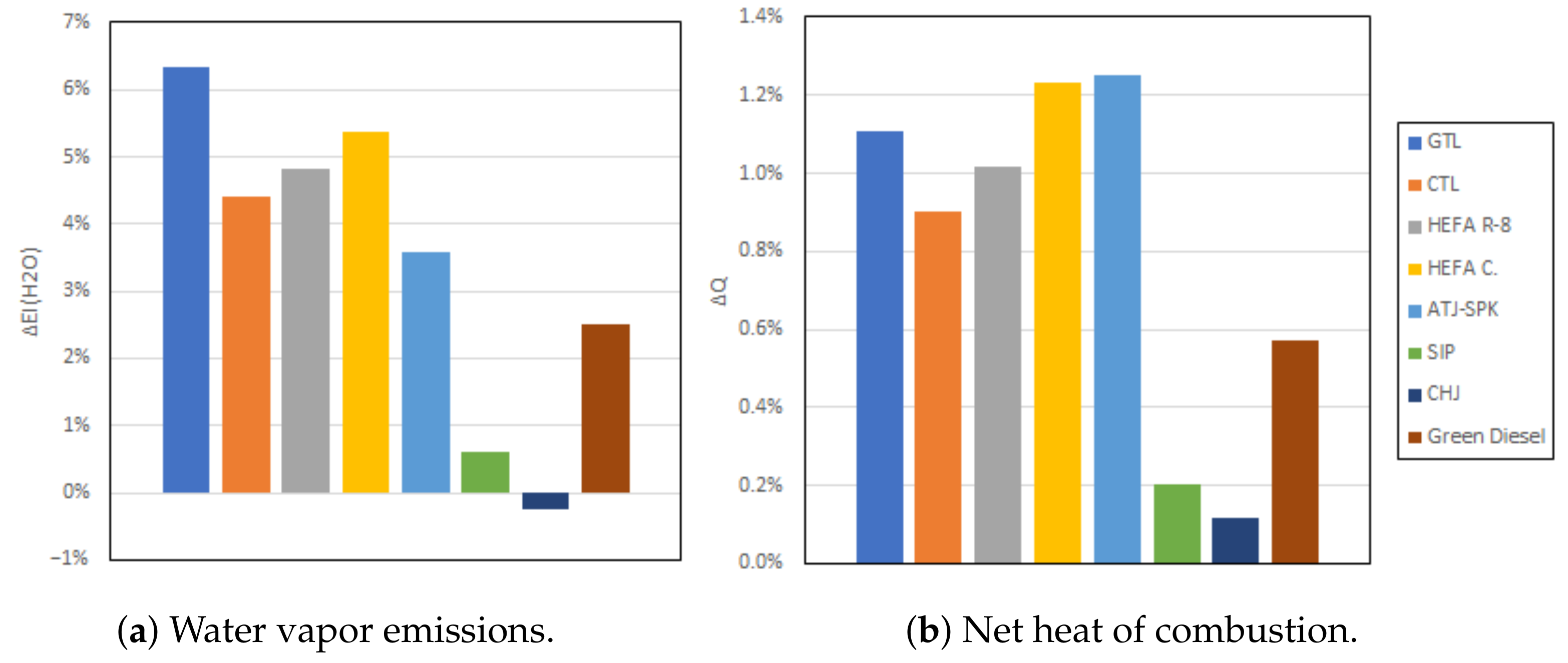
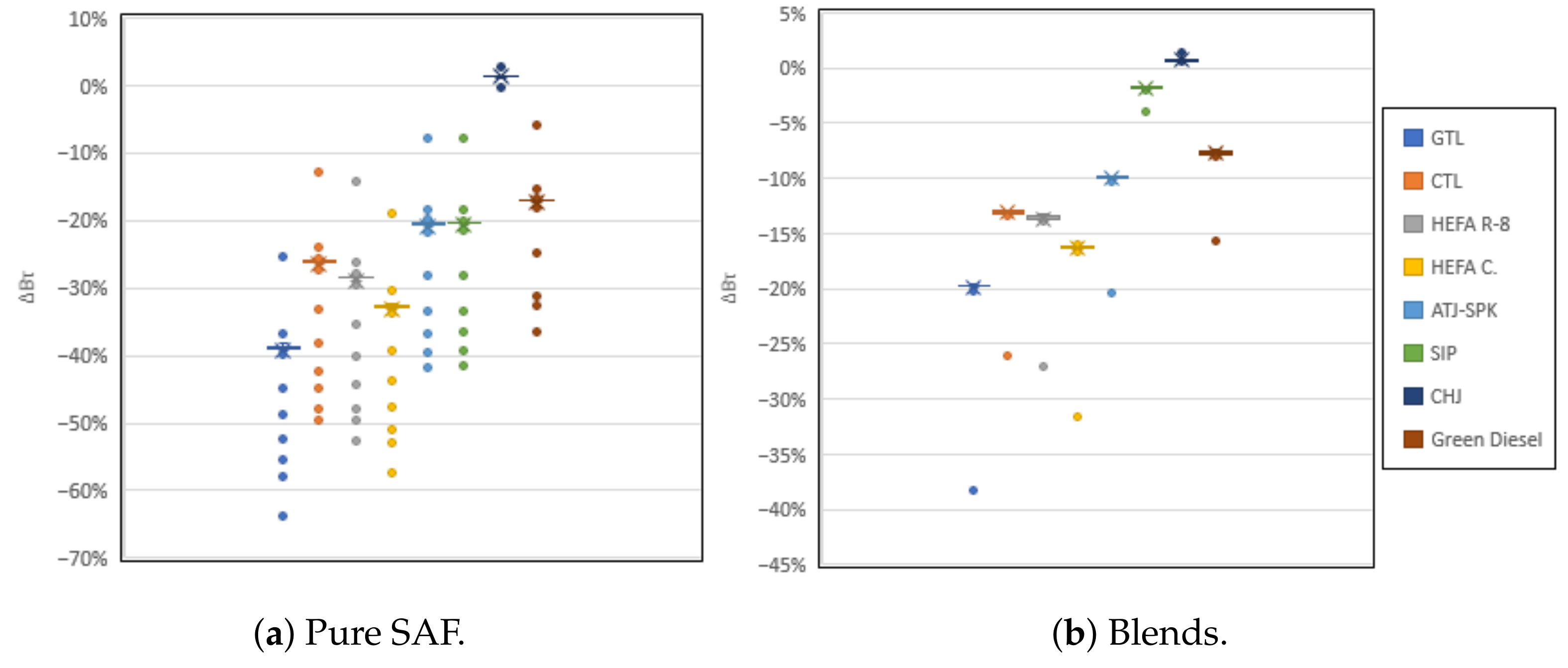
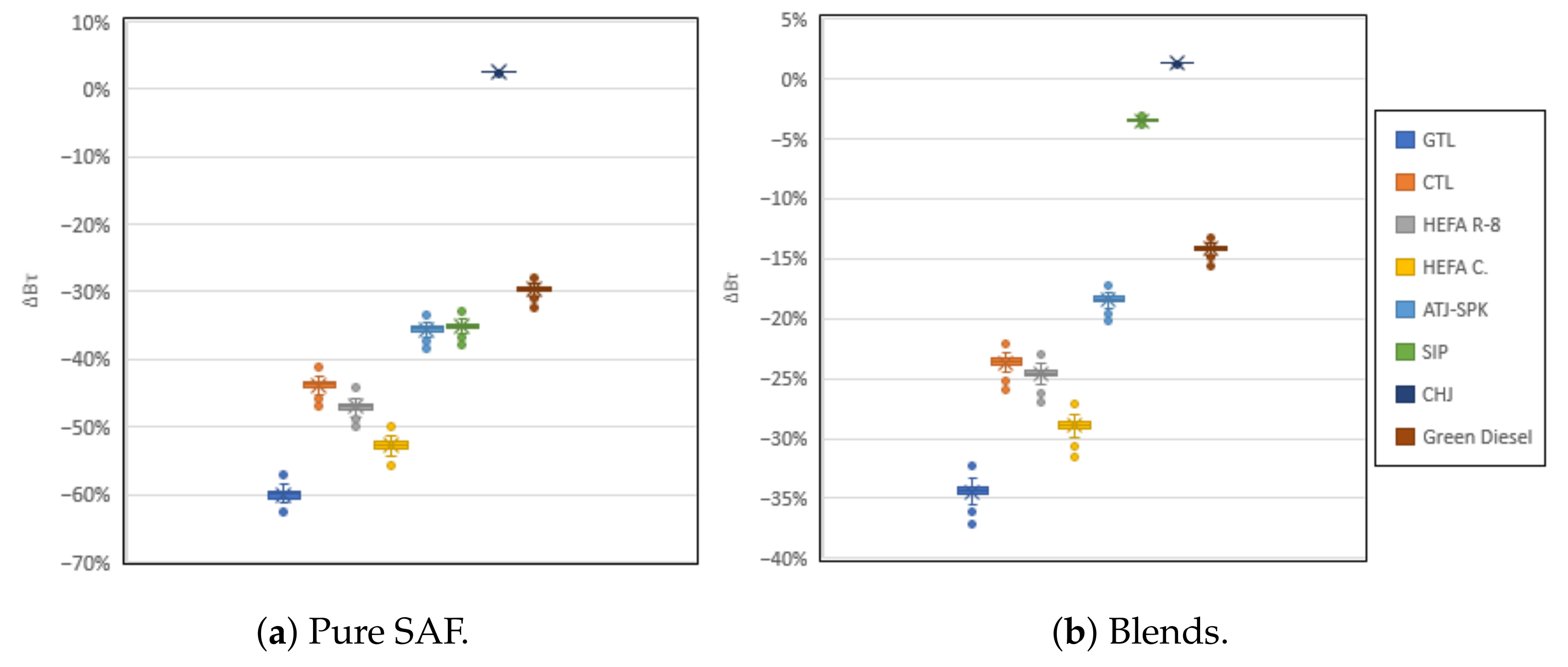
Figure 4 shows the RDs in water vapor emissions and net heat of combustion for the various SAF considered in the present study. These are presented here to contextualize the contrail formation frequency results.
An increase in water vapor emissions aids the formation of contrails, while an increase in net heat of combustion hinders it. While both the water vapor emissions indices and net heat of combustion increase for all SAF (except for CHJ, which has higher net heat of combustion and a lower water vapor emission index than Jet A-1 fuel), the increase in water vapor emissions is much greater.
The values for blends, shown in
Figure 5, follow the same trend as those for pure SAF, but with less marked differences. As stated previously, all blends have a SAF ratio of 50% except for SIP which is mixed in at 10%; this is the reason for the much smaller RDs found for the SIP blend when compared to pure SIP.
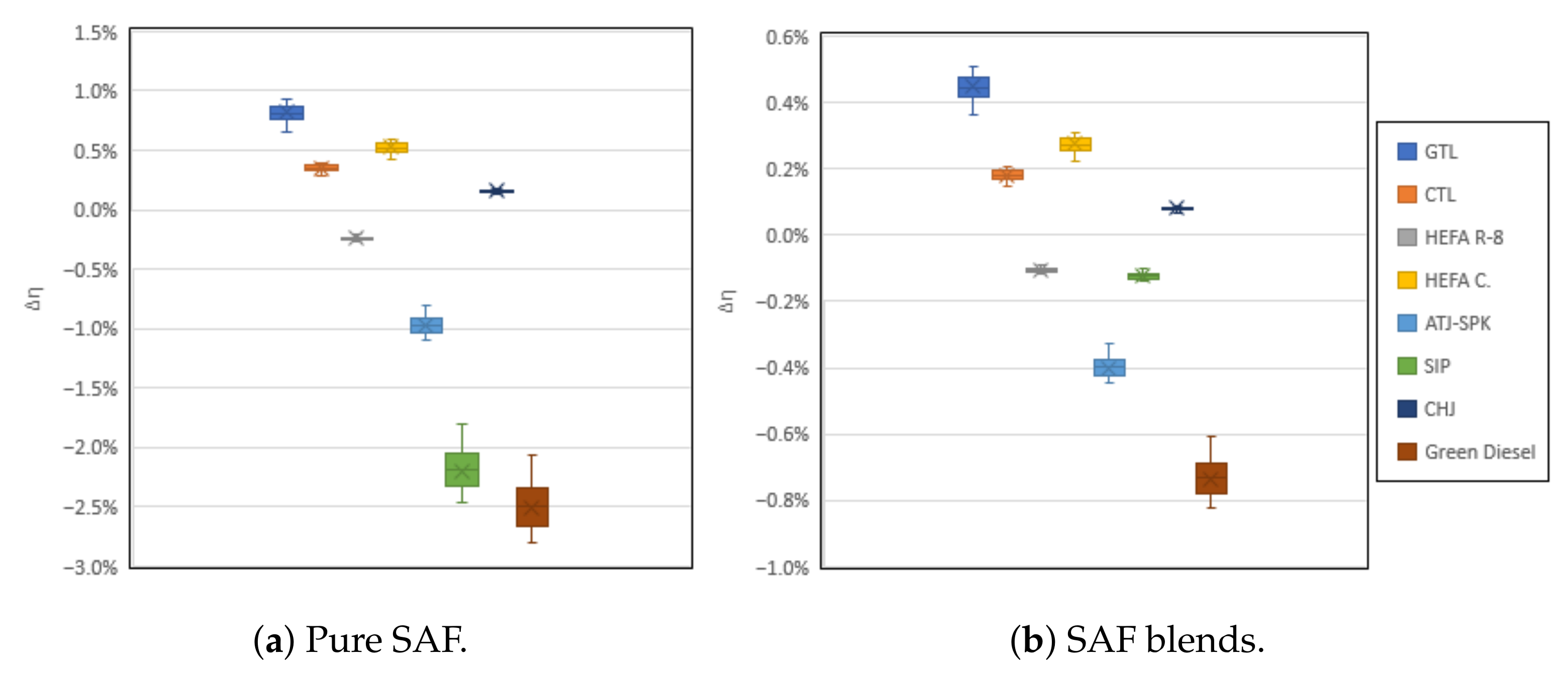
Figure 6 shows the RDs in propulsive efficiency for the different SAF and SAF blends. The use of GTL, CTL, HEFA C., and CHJ provides a small increase in propulsive efficiency, while burning the other fuels results in a small decrease. The propulsive efficiency is directly influenced by the net heat of combustion of the fuel, and indirectly influenced by a number of fuel properties during the combustion. While the latter can not be fully isolated from each other, it appears that the boiling point of the different fuels holds the greatest weight. During combustion, a higher fuel boiling point will lead to a lower combustion efficiency, which seems to be the main differing factor between the fuels. Still, the differences found in propulsive efficiency are small enough to be mostly inconsequential in the study.
An increase in contrail formation frequency was expected due to the increase in water vapor emissions typical of SAF combustion, and this was indeed the case. The increase in the net heat of combustion, which could hinder this frequency increase, is far outshone by the differences in water vapor emissions. As expected, the small decrease in propulsive efficiency experienced by some fuels (or increase in propulsive efficiency for CHJ) does not alter the trend set by the water vapor emissions either.
The increase in contrail formation frequency happened right behind and after Jet A-1 contrail formation areas; that is to say, in route segments where contrails formed for all fuels, contrails were formed for most SAF slightly earlier (with contrails forming for CHJ slightly later).
There were no contrails formed for SAF outside of these conditions. In routes where contrails were not formed for Jet A-1, they were also not formed for the other fuels, and there were no isolated segments of contrails formed for SAF only. In other words, this increase in contrail formation frequency resulted in slightly longer contrails, and not in new separate contrails.
An increase in frequency of under 1% for the different fuels was found. This is better represented by the differences in the contrail formation threshold temperature.
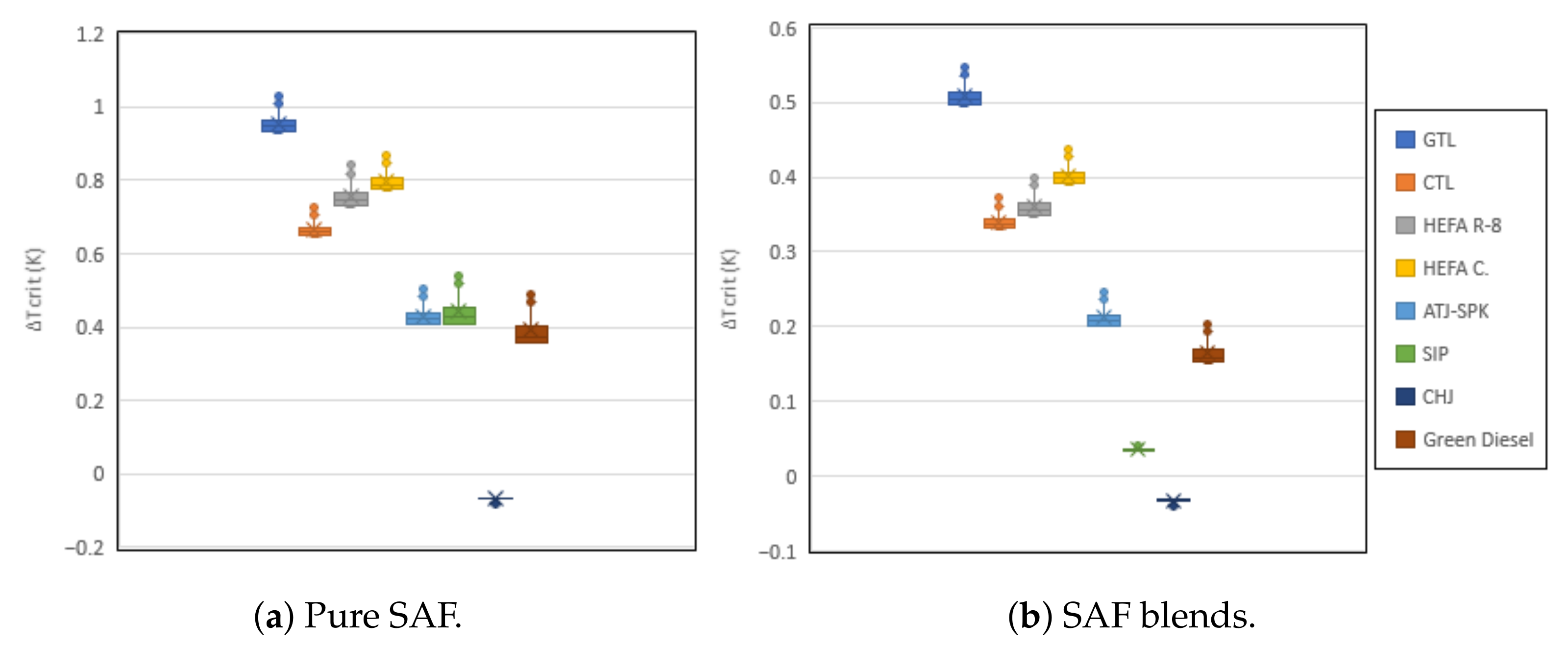
Figure 7 represents the absolute differences in threshold temperature for pure SAF and SAF blends. As stated previously, contrails form when the ambient temperature is below the calculated threshold temperature for that location. As can be seen from the plots, the contrails for the different SAF will form at temperatures within approximately 1 K or less from each other. While it is not impossible for isolated segments of SAF contrails to exist, the small difference in temperature explains why the frequency increase resulted only in longer contrails; it is unlikely for aircraft to reach SAF threshold temperatures without crossing to one degree under.
Comparing the values for ATJ-SPK and SIP in
Figure 7a, it can be seen that while water vapor emissions control the trend, the small differences in the net heat of combustion of the fuels do hold an observable influence over the formation frequency; despite the similar water vapor emission indices between these fuels, SIP has a lower net heat of combustion which results in slightly higher threshold temperatures.
3.2. Contrail Lifetime
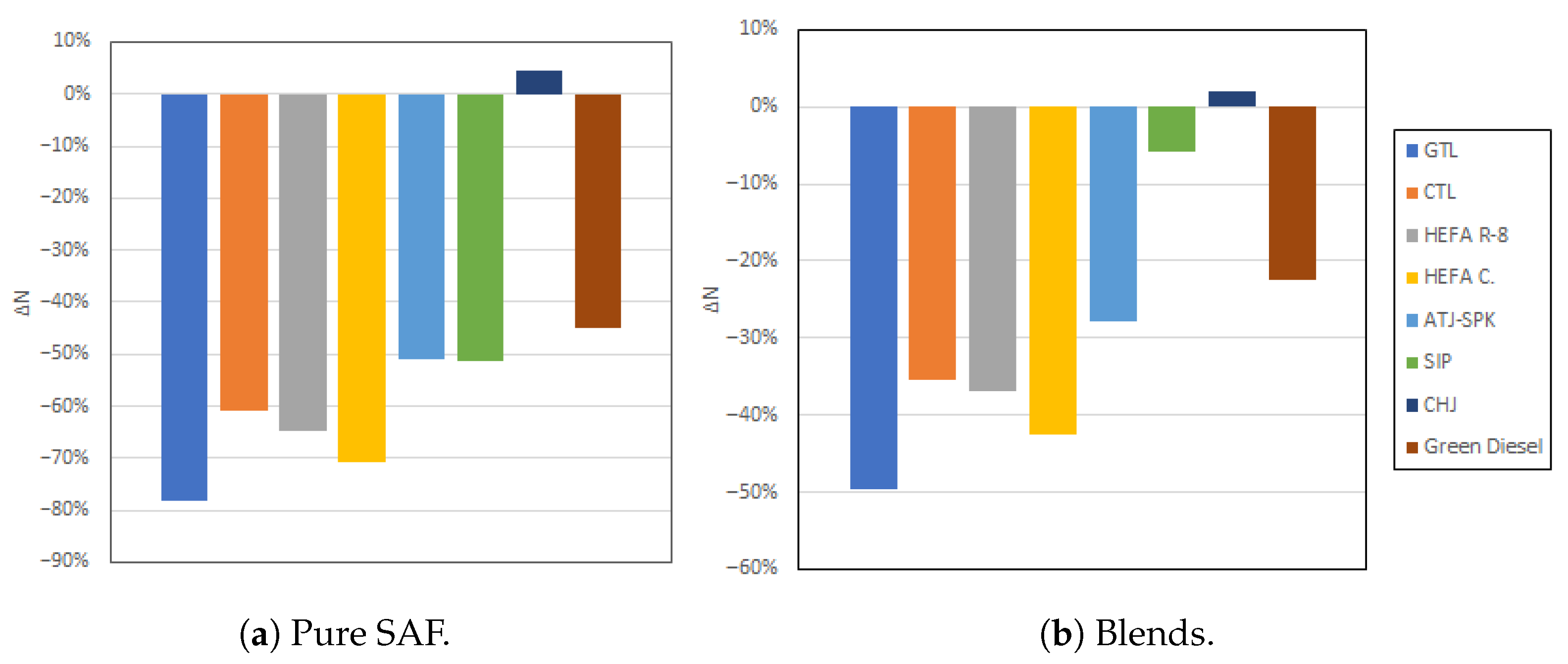
Figure 8 shows the Mean Relative Differences (MRDs) in particle number emissions between the different SAF and Jet A-1 fuel. These are shown in a bar plot, and not a box-and-whisker plot, due to the very low dispersion found in the results; this is due in part to the limited variation in flight conditions, but also possibly due to the previously expanded upon limitations of the soot prediction model used.
The main fuel-dependent factors influencing contrail properties are the water vapor emissions and the particle number emissions. All fuels show the same trend—an increase in water vapor emissions and decrease in particle number emissions—except for CHJ. To avoid redundancy, when SAF behavior is described in this section, it will be referring to all SAF with the exception of CHJ, with the implication that CHJ is displaying the opposite behavior.
The contrail lifetime analysis is split into three parts due to the large deviation in values found between these: contrails with lifetimes of up to 30 min, contrails with lifetimes ranging from 30 min to 2 h, and contrails with lifetimes greater than 2 h.
The general trend was that the higher the reference contrail lifetime was, the higher the decrease in lifetime for SAF contrails occurred, with young contrails experiencing an increase in lifetime instead. However, this was not a direct correlation. The lifetime of each contrail is heavily dependent on the surrounding environment during its lifetime, which leads to a large deviation in the RDs for reference contrails with very similar lifetimes.
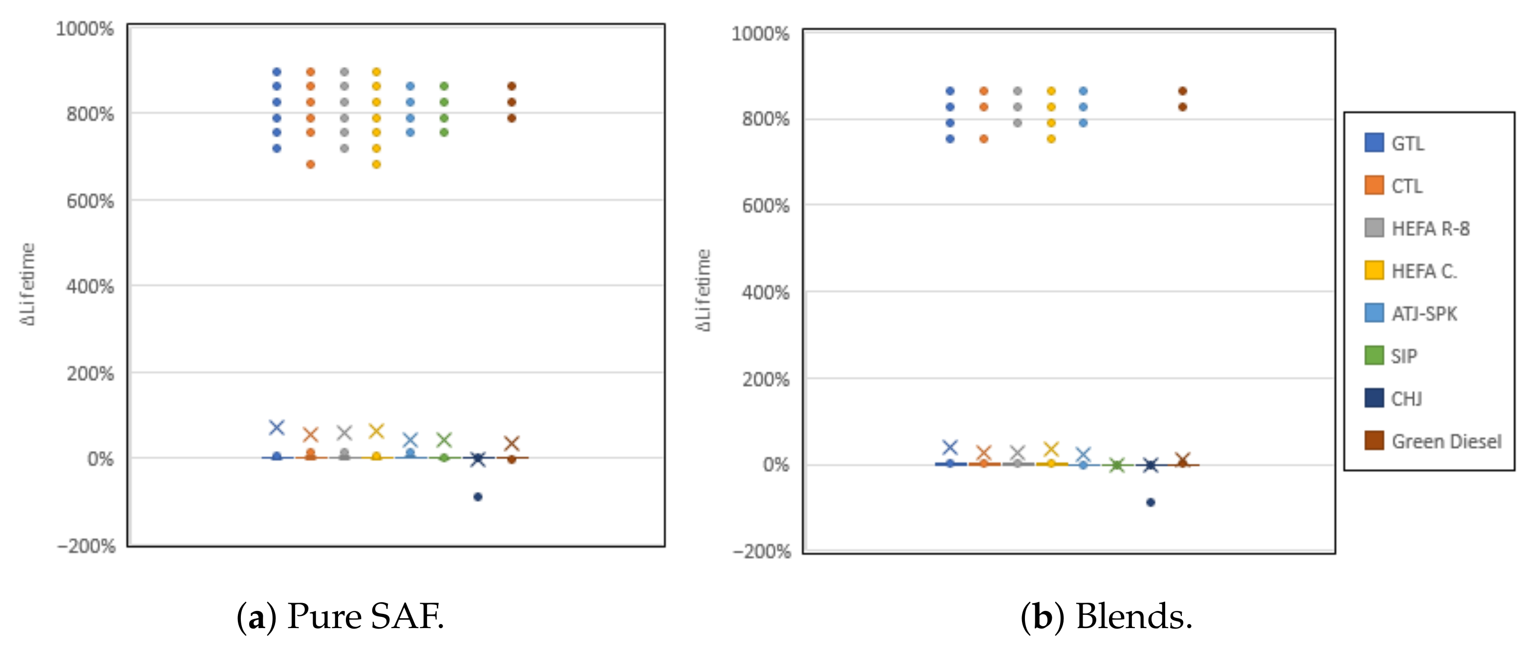
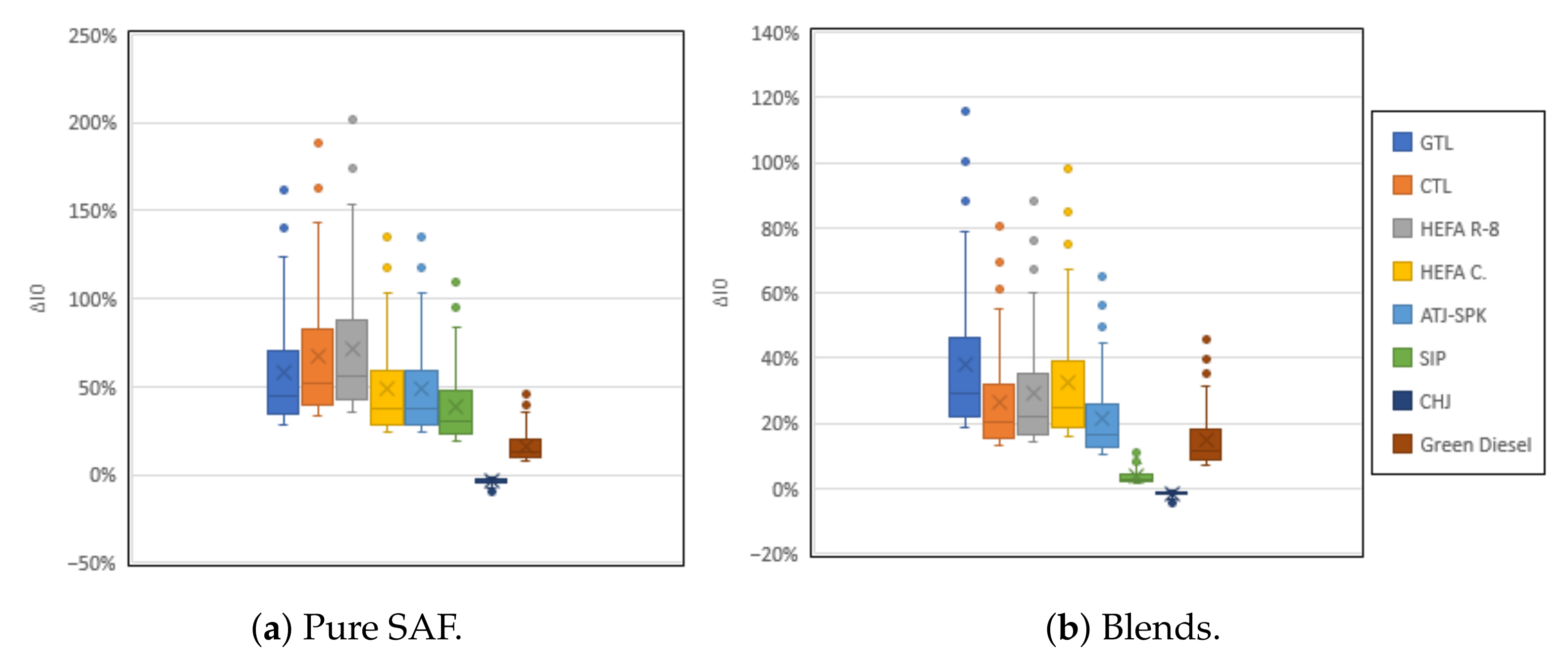
Figure 9 shows the RDs in lifetime for the cases where the reference contrail, that is, the contrail formed when Jet A-1 was burnt, had a lifetime of 30 min or less. For this time range, contrails almost always ended due to their ice mass reaching zero; this was not the case for longer lasting contrails, which typically ended due to reaching very low optical depths despite still having a positive ice mass. The key fuel-dependent factor controlling the contrail lifetime for this time range is thus considered to be the water vapor emissions index.
Most contrails in this time range have RDs in lifetime close to 0%, but the MRDs are dragged up due to the very high outliers. These outliers were all present in the same short segment and seem to be the result of SAF contrails reaching higher relative humidity areas shortly after the reference contrail lost its ice mass. The plot for the blends, cf.
Figure 9b, presents less outlier points, with the 10% SIP blend showing no outlier points in the 800% at all, despite pure SIP presenting the same number of outliers as ATJ-SPK; this is due to the SAF blend contrails, closer in properties to the Jet A-1 contrails, evaporating before the higher relative humidity areas as well.
There is a high deviation in the results for this time range even within the same few seconds; the highest RDs were found for reference contrails aged around 46 s, but other contrails of around the same age led to RDs of close to 0%.
At around the 20 min mark, the lifetime of SAF contrails starts decreasing instead of increasing with respect to that of the reference contrails; this transition zone differs among the different fuels. Small decreases for SAF contrail lifetime were found as early as 14 min for GTL and HEFA C.; at around 23 min for HEFA R-8, SIP, and Green Diesel; and at around 27 min for CTL and ATJ-SPK. Small increases for SAF contrail lifetime were found as late as 27 min for GTL; 20 min for CTL, HEFA R-8, HEFA C., and ATJ-SPK; and 13 min for SIP and Green Diesel.
Contrails with lifetimes in this transition zone were still formed in dry-enough areas that their water content was the main driving force for the differences; both SAF and conventional contrails evaporated early in their lifetimes, with the higher water content of the SAF contrails allowing them to live longer. Beyond this range, soot particle emissions control the trend; while some contrails still sediment into drier zones and evaporate, the lifetimes of most contrails end due to these becoming extremely optically thin with time.
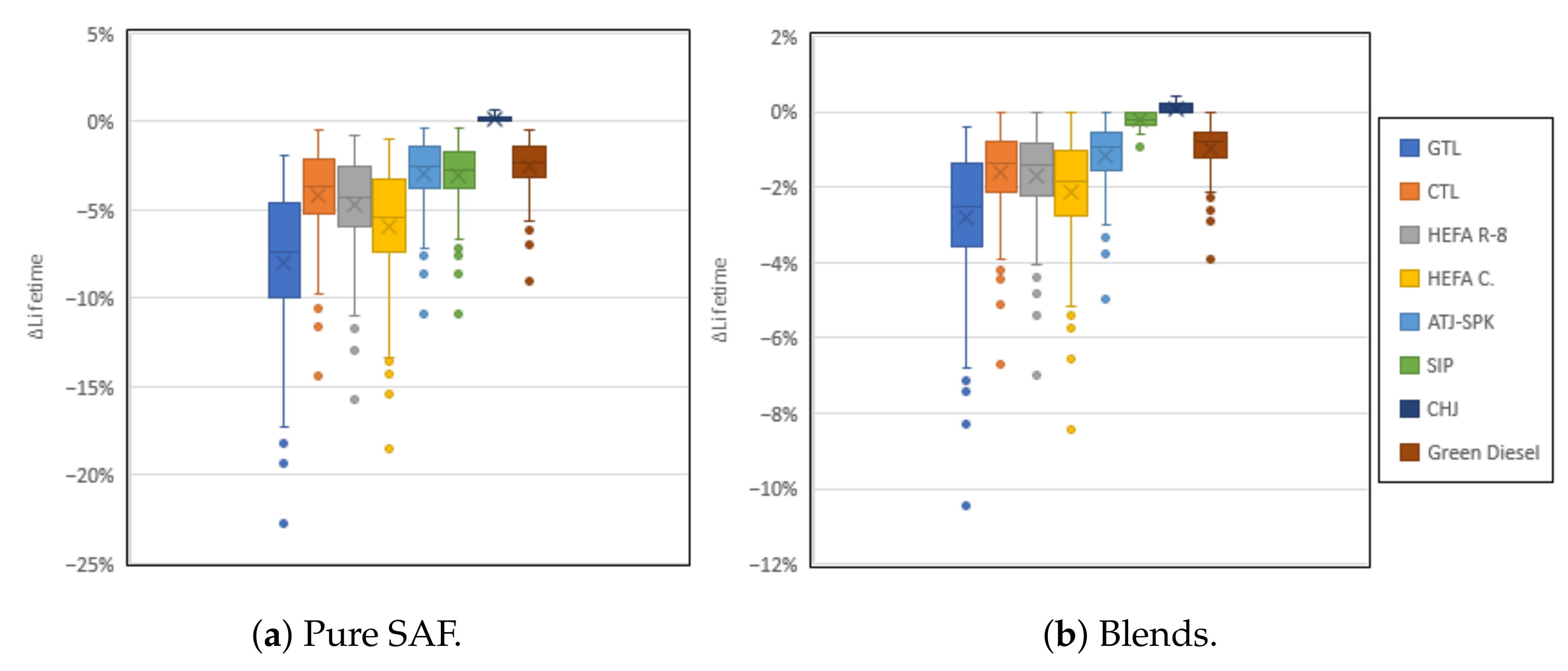
Figure 10 shows the RDs in lifetime for reference contrails with lifetimes up to 2 h. From the 27 min mark, when the last lifetime increase was found, all SAF contrails ended earlier than the reference contrails at the same point. Results in this range still show some dispersion for reference contrails lifetimes that are close to each other, but there is a clear trend of higher reference lifetimes yielding higher RDs. The outliers in this range are all found for 80 min or above, but, for this same range, values inside the IQR were still found.
Note that while RDs pale in comparison to those found for the previous time range, absolute differences are not that far apart. The outliers in
Figure 9, with increases of over 800%, correspond to absolute differences of a little less than 4 min, while mean values for this range correspond to absolute differences of around 1 min for the SIP blend to 5 min for GTL.
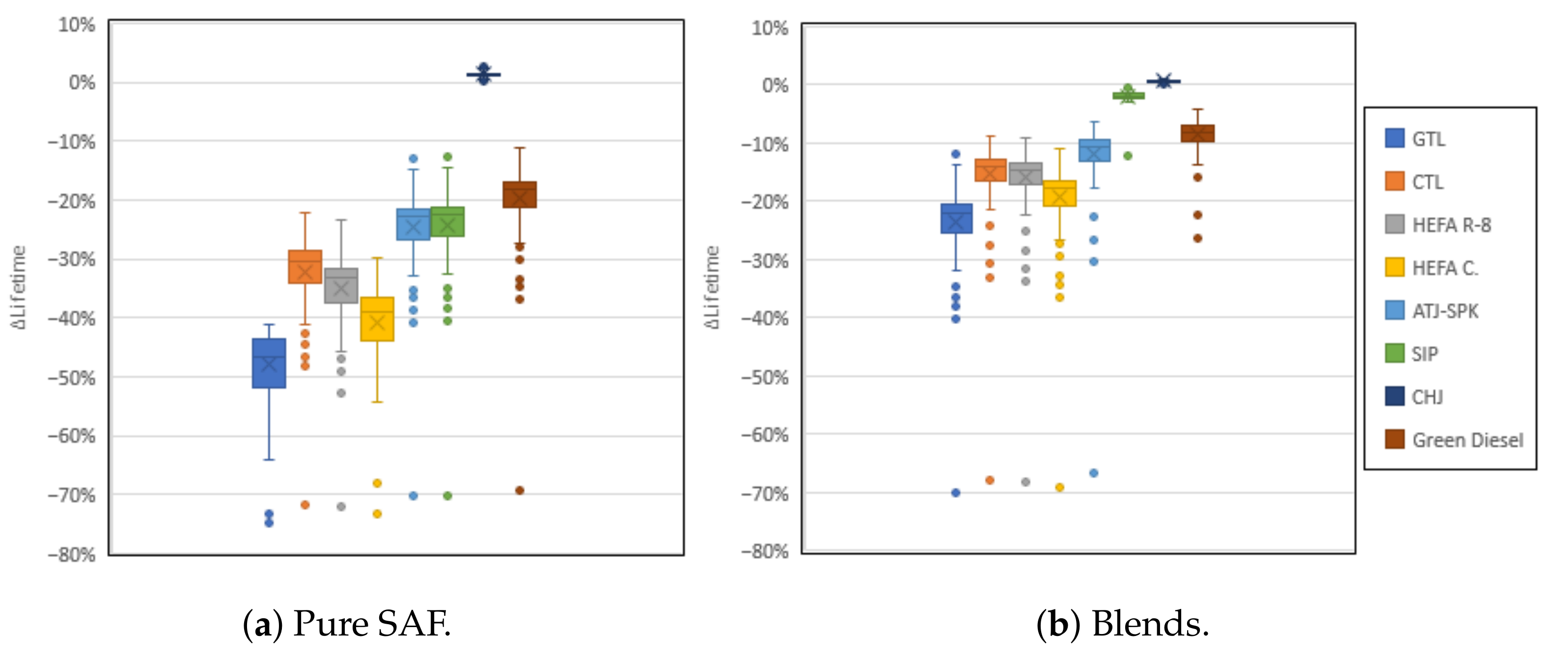
Figure 11 shows the RDs in lifetime for reference contrails with lifetimes of over 2 h, with the oldest contrails exhibiting lifetimes somewhat over 11 h. This range represents the typical contrail cirrus lifetime, and, much like the previous range, it shows a trend of sharper decreases for higher reference contrail lifetimes.
The maximum RDs, represented by the outliers at approximately −70%, were found for a reference contrail with a lifetime of around 7 h, resulting in an absolute difference of slightly over 5 h for pure GTL. This did not correspond to the highest absolute difference, which was of 6 h and 20 min for pure GTL and occurred for a reference contrail with a lifetime of 10 h and 40 min.
3.3. Optical Depth and Radiative Forcing
The climatic impact of a contrail cirrus is controlled by the product of its width by its optical depth. While the optical depth of a contrail is highest for young contrails, this product increases with contrail age, typically reaching maximum values a few hours into a contrail’s lifetime. This makes contrail cirrus, which have much higher lifetimes, responsible for the largest climatic impacts [
20].
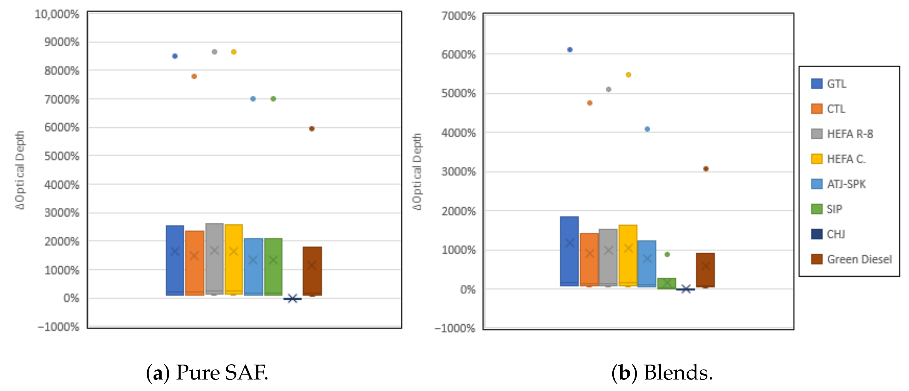
The optical depths immediately after the wake vortex are analyzed here first. These are the peak optical depths values for these contrails, found at typical lifetimes of less than a minute. To account for the large dispersion in the results, these are split into different plots according to the local humidity at formation. It could be seen that both the particle number and the ice mass of the contrail heavily influenced the results; to contextualize the results, plots of the RDs for initial ice mass ratios are included.
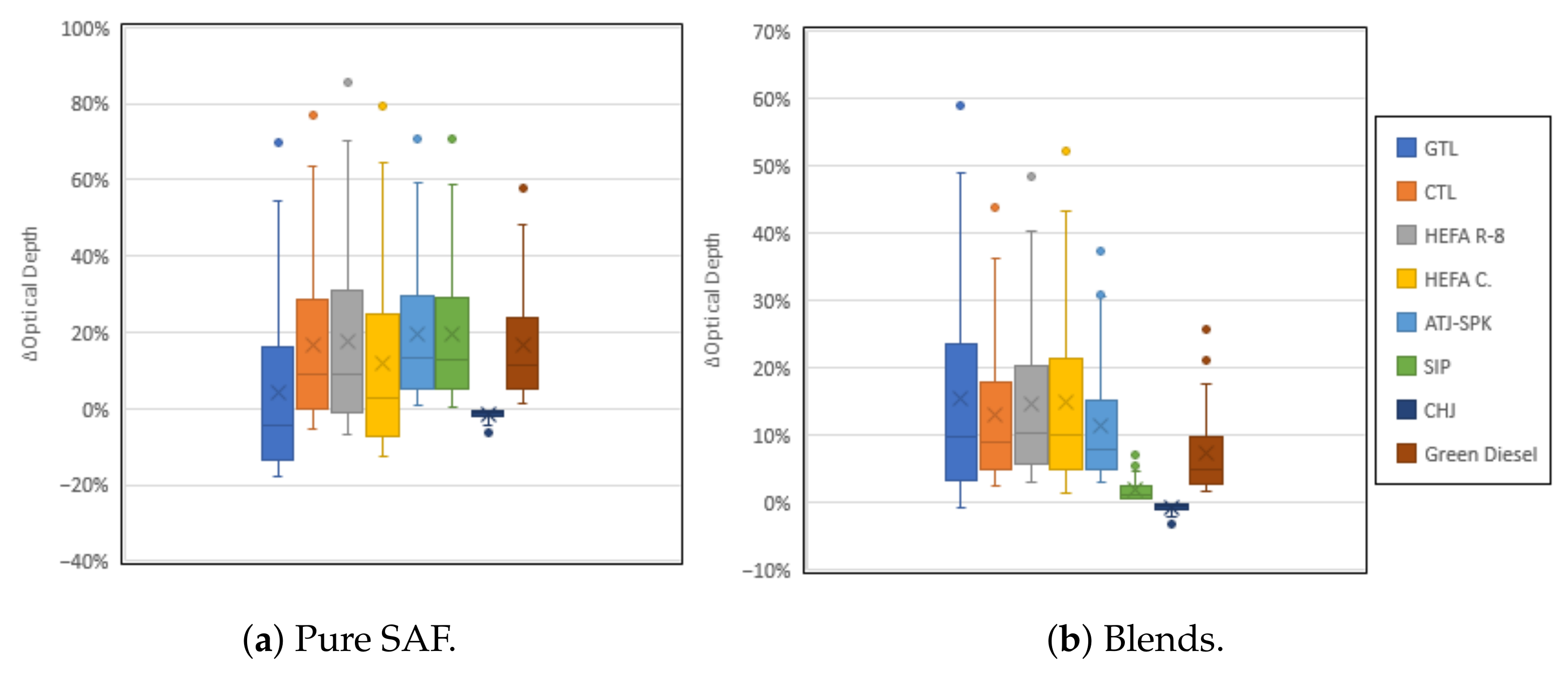
Figure 12 shows the bulk of results; these were optical depths for contrails formed in environments with a relative humidity of 43% or higher.
The optical depths found in this range had typical values of 0.1–0.5, and the RDs between fuels seemed to be mostly influenced by the particle emissions. The results showed a relatively small deviation, with IQRs of 2% or less. Still, there was a trend of a reduction in ambient relative humidity at formation leading to smaller RDs, typically associated to lower reference contrail optical depths. The outliers plotted all correspond to contrails formed at relative humidities lower than 50%.
Contrails formed in these humidities tended to have higher initial ice mass fractions, typically in the order of 10
−5. As seen in
Figure 13, while the MRDs of each fuel tend to follow the trends set by the water vapor emissions, a large dispersion can be seen, with outliers that do not always respect this.
The optical depth of contrails formed in this range of humidity appear to be mostly influenced by soot particle emissions, with the ice water content of the contrail holding no visible influence.
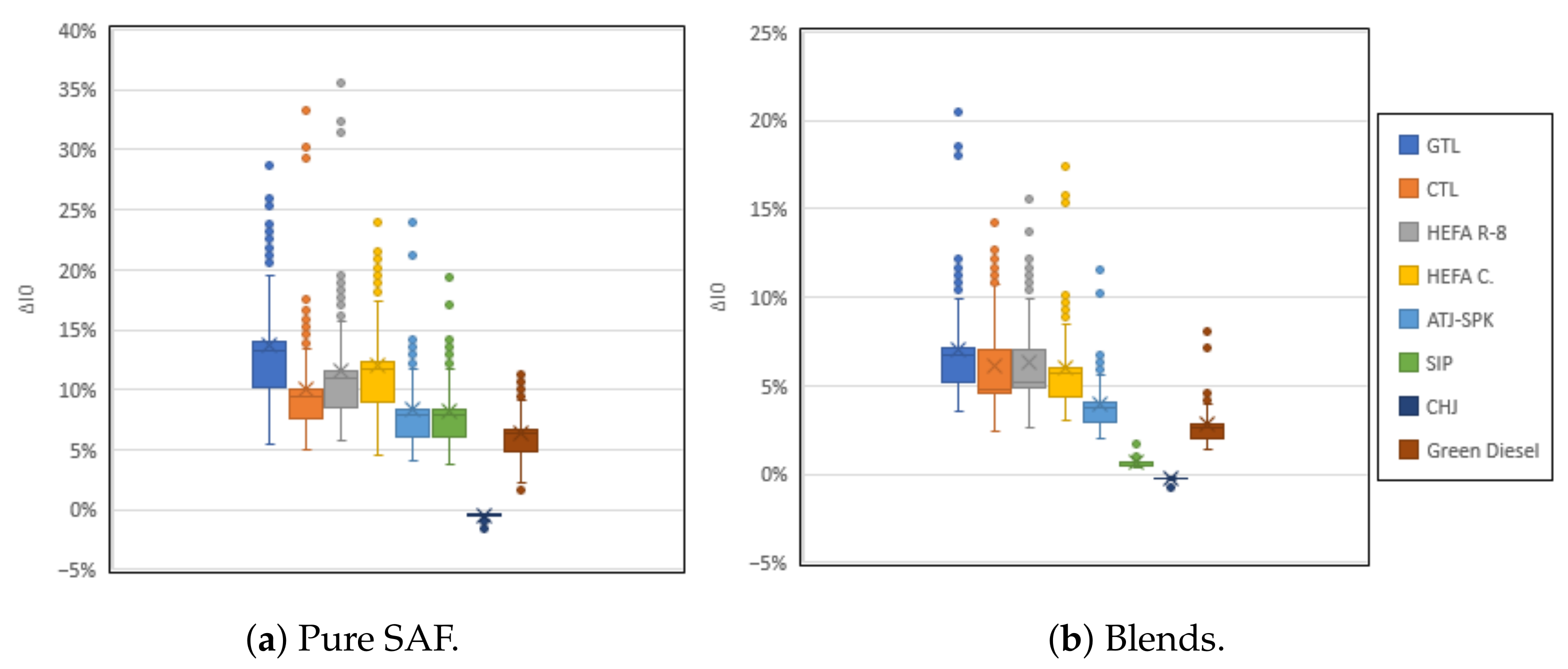
Figure 14 shows the RDs for contrails formed at relative humidities of 41% to 43%. Fewer contrails were formed in these conditions, and those formed had peak optical depths in the range of 0.02 to 0.1. Optical depths in this range are not visible in satellite observations and should have limited climatic impact.
The different SAF started yielding positive RDs for different relative humidities; GTL at a relative humidity of approximately 42%, HEFA C. at about 42.5%, CTL and HEFA R-8 at around 42.7%; and the other fuels, including CHJ, which started yielding negative RDs instead of positive RDs, at approximately 43%. In the case of blends, all led to increases starting at a relative humidity of around 43%.
As seen in
Figure 15, initial ice mass ratios for this range were typically of the order of 10
−6, and their influence in the optical depth is much clearer here than in the previous range. Peak RDs in optical depth can be seen to directly correspond to peak RDs in ice mass ratios. The highest MRD in optical depth was found for pure HEFA R-8, corresponding to the highest MRD in initial ice mass ratio as well. Nevertheless, soot particle emissions still held some influence for contrails in this range.
Contrails formed at relative humidities of 40% or less fully lost their ice content during the wake vortex phase, and so optical depths for these were not calculated. A few contrails were formed for the relative humidity range of 40% to 41%. Jet A-1 contrails formed in this range had optical depths of 0.0003–0.02, while SAF optical depths reached peak values of approximately 0.04; these are all very optically thin contrails that should produce a negligible climate impact. RDs in optical depth for this range are shown in
Figure 16.
There were very few reference contrails formed under these conditions, and all had initial ice mass ratios in the order of 10
−8–10
−7.
Figure 17 shows the RDs in initial ice mass ratios for the different SAF in relation to Jet A-1 fuel; it is quite clear that the ice mass ratios control the differences in optical depth in this range. These optically thin contrails have very small ice contents (almost null), so even small differences in water vapor emissions can increase their optical depth a few orders of magnitude; nevertheless, even the SAF contrails in this range can be considered extremely optically thin.
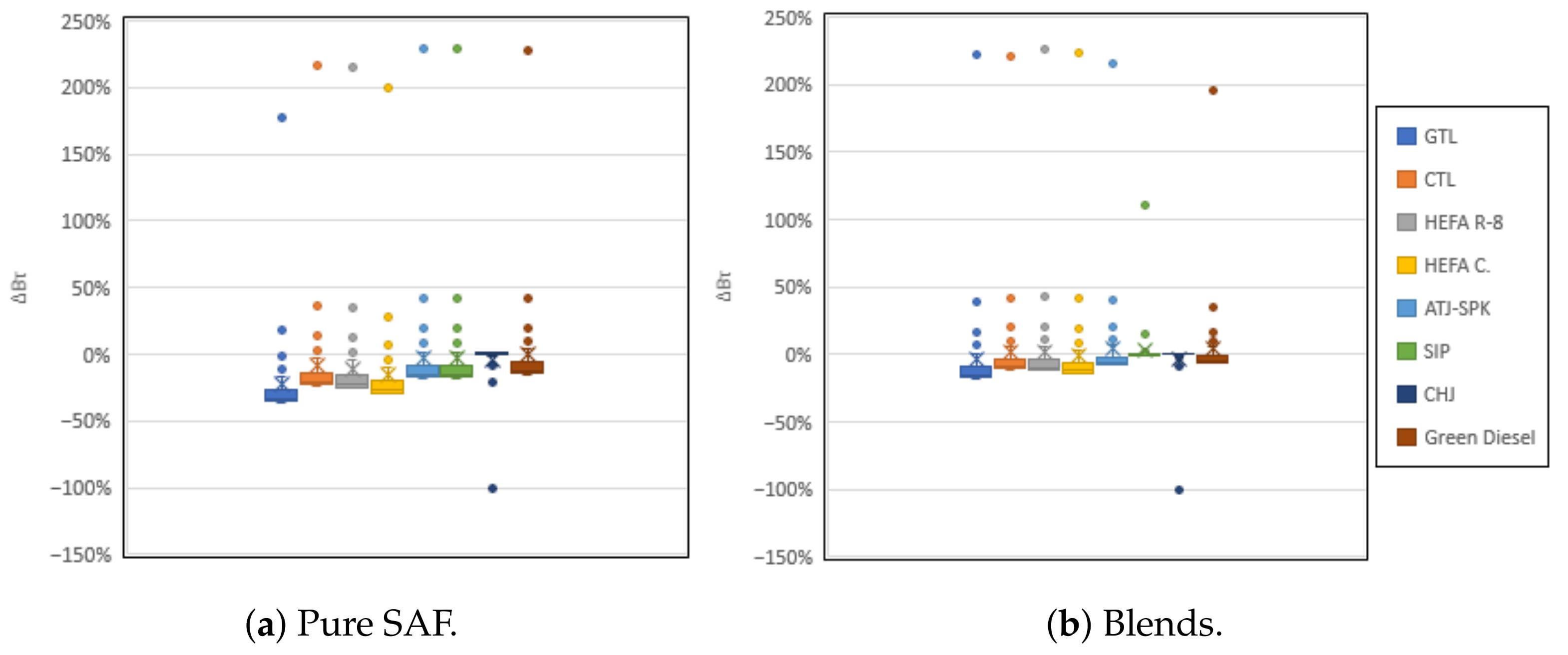
As stated previously, the RF of contrails is controlled by the product of contrail width by optical depth. This value tends to reach its peak not for young contrails, but for contrail cirrus with a few hours of age. The influence of the different fuels on this product is analyzed for the peak value corresponding to each contrail, which for contrails with long lifetimes may mean that values with a few hours of difference are being compared. The values analyzed here are thus not only influenced by the optical depth of the contrail, but also by the contrail’s lifetime.
Figure 18 shows the RDs in the product of the contrail width by optical depth for a relative humidity range of 43% to 58% at formation; this is the range containing the bulk of the results. While the IQR for these plots is very small, about 1%, there is a high amount of outliers for pure SAF. This is due to the influence of the contrail lifetimes; while most contrails formed in these conditions have similar lifetimes, some contrails settle into more humid locations and end up living far longer.
As previously seen, long-lasting contrail cirrus experience much bigger decreases in lifetime than younger contrails (pure GTL had a MRD of −47.94% for reference contrails aged 2 h or more and a MRD of −8.02% for contrails aged under two hours), which leads to SAF peaks being reached much later in relation to Jet A-1 contrails, enhancing the differences in this way.
Contrails formed at an ambient relative humidity of 58% or above all led to long-lasting contrail cirrus. The RDs for the product of width by optical depth is shown in
Figure 19 separately from the previous range to illustrate the low dispersion.
This range contains contrails with large RDs in peak optical depth value, and absolute differences in lifetime of a few hours. The effect of the contrail age on this product is most clearly felt here. As the product of contrail width by optical depth is the factor which controls a contrail’s RF, the biggest impact on the climatic influence of contrails when using SAF should be felt for contrail cirrus and not young contrails.
Figure 20 shows the RDs for the contrails formed at a relative humidity of 40% to 43%. Below a relative humidity of 40%, as stated before, all contrails dispersed during the wake vortex phase and thus no calculations are presented.
Contrails formed in this range had peaks at less than one minute of age. Accordingly, the peak optical depth and the optical depth at the peak of the product of contrail width by the optical depth were very close to each other. Adding to this, the largest influence on the width of a contrail at these times is the size of the aircraft, which makes the widths between the different fuels also quite similar. This led to a RD trend which was mostly controlled by the peak optical depths.


