Simulation of Optimal Driving for Minimization of Fuel Consumption or NOx Emissions in a Diesel Vehicle

Abstract

Significant reduction in fuel consumption and NOx emissions can be achieved just by changing the driving along the road. In this paper, dynamic programming is employed to find two different driving profiles optimized for fuel consumption and NOx creation minimization in a diesel vehicle. Results, show that the fuel reduction driving cycle leads to fuel savings of 4% compared with the average consumption with arbitrary driving. The NOx reduction driving profile improves the emissions of arbitrary driving by a 34.5%. NOx oriented driving profile improves the emissions of the fuel-oriented cycle by a 38% at the expense of a fuel consumption penalty of 10%. This result points out the difficulty of a simultaneous NOx and fuel consumption reduction, stressing the efforts to be done in this field during the following years. Strategies followed and conclusions drawn from this paper are relevant concerning vehicle autonomy integration.

1. Introduction

The increasing number of vehicles on the road represents a large part of the global energy consumption. To avoid the shortcomings of cycles with a vehicle test bench under a climatic chamber [1,2], such as the NEDC (New European Driving Cycle), there are new homologation cycles, such as the RDE (Real Driving Emissions) cycle.

These cycles highlight the effects of real urban, extra urban and rural driving in terms of pollutant emissions for light-duty [3] or heavy-duty vehicles [4]. The current tendency in new developments of internal combustion engines is to make engines more adiabatic [5], increasing the indicated work and the exhaust flow enthalpy, which can be later recovered via thermoelectric generators [6,7,8] or Organic Rankine Cycles [9,10]. Other trend is the hybridization of vehicles [11,12].

A different approach to reduce energy consumption of vehicles without changes in its components is the driving velocity profile optimization. The driving style, together with road geometry and altitude, have a huge impact on fuel economy. Driving style has been characterized by the driving speed acceleration and deceleration, lateral acceleration and regenerative braking efficiency. The acceleration percentage rate and speed oscillations also characterize the driving style [13].

Optimization-based control algorithms have been used to obtain vehicle velocity profiles so that the fuel consumption is reduced. For instance, Asadi and Vahidi [14] proposed an algorithm to guarantee that a vehicle approaches traffic lights at green when possible using short range radar and traffic signal information. An optimum velocity profile was scheduled for a timely arrival at green traffic light with minimal use of braking, maintaining safe distance between vehicles. This strategy was able to reduce fuel consumption by 47% for simulated driving through a sequence of 9 traffic lights.

Wadud et al. [15] considered that a 20% reduction in fuel consumption is possible only by replacing common driver strategies with a set of energy-saving practices, which is commonly known as eco-driving.

In Zavalko [16], truck drivers were trained in eco-driving. As a result of the training, reduction of fuel consumption by 13.6% in average was achieved. Long-term effect of the training was moderate (4% reduction in fuel consumption 3 months after the training).

One approach is to drive in a way that engines can spend as much time as possible at its most efficient operating points, which typically means high load and moderate speed. Another is to minimize the energy losses produced by braking, by decreasing the number of breaking-acceleration cycles [17].

Mensing et al. [18] studied an optimized drive cycle to reduce fuel consumption for a light-duty vehicle. In their work, they show a 16% reduction with respect to the New European Driving Cycle (NEDC), maintaining travel time and respecting speed limits. When compared with a more realistic driving cycle, the potential reduction was found to be around 34%. The potential of driving profile optimization drops to 10% in the case of hybrid electric vehicles in realistic driving conditions. The reason for this is that hybridization enables regenerative braking and the advantages of avoiding acceleration-braking cycles decrease [19].

Wegener et al. [20], used deep reinforcement learning for automated eco-driving in urban scenarios. Energy savings of up to 19% were found compared with a simulated human driver. Hellström et al. [21] developed a fuel-optimal control for a heavy-duty diesel truck taking advantage of information of the road topography ahead of the vehicle when the route is known. The trial route was a 120 km segment of a Swedish highway. In average, the fuel consumption was decreased about 3.5% without increasing the trip time.

Most of the literature surveyed, only consider fuel consumption, and ignore NOx emissions. Unluckily, strategies to reduce fuel consumption usually lead to an increase NOx production. This paper aims to increase the awareness on this trade-off effect. In particular, the target of this work is to explore the impact of driving conditions on the fuel consumption and emissions by comparing real driving with the optimal speed profiles to minimize fuel consumption and NOx in the same route while keeping the same trip time. Two optimal driving profiles were derived by the application of Optimal Control theory: one optimal for fuel consumption and the other optimal for reducing NOx emissions. The differences between natural, fuel optimal and NOx optimal driving strategies are examined and the impact on fuel consumption on NOx emissions are showed. Results point out that due to the NOx and fuel consumption engine map shapes, natural driving approaches the optimal fuel consumption trajectory, while NOx minimization involves a substantially different driving pattern, which could be relevant for autonomous driving integration.

2. Materials and Methods

The methods described in this section were applied to driving strategies of a diesel Nissan X-Trail. First, an engine mapping in a test-bench was done to obtain data of representative parameters under any engine requested output. Later, a characterization of a selected route in terms in altitude above sea level and maximum permitted speed (from driving regulations) was done. The optimization method provided the optimum driving profile on the selected route to minimize fuel consumption or engine out NOx.

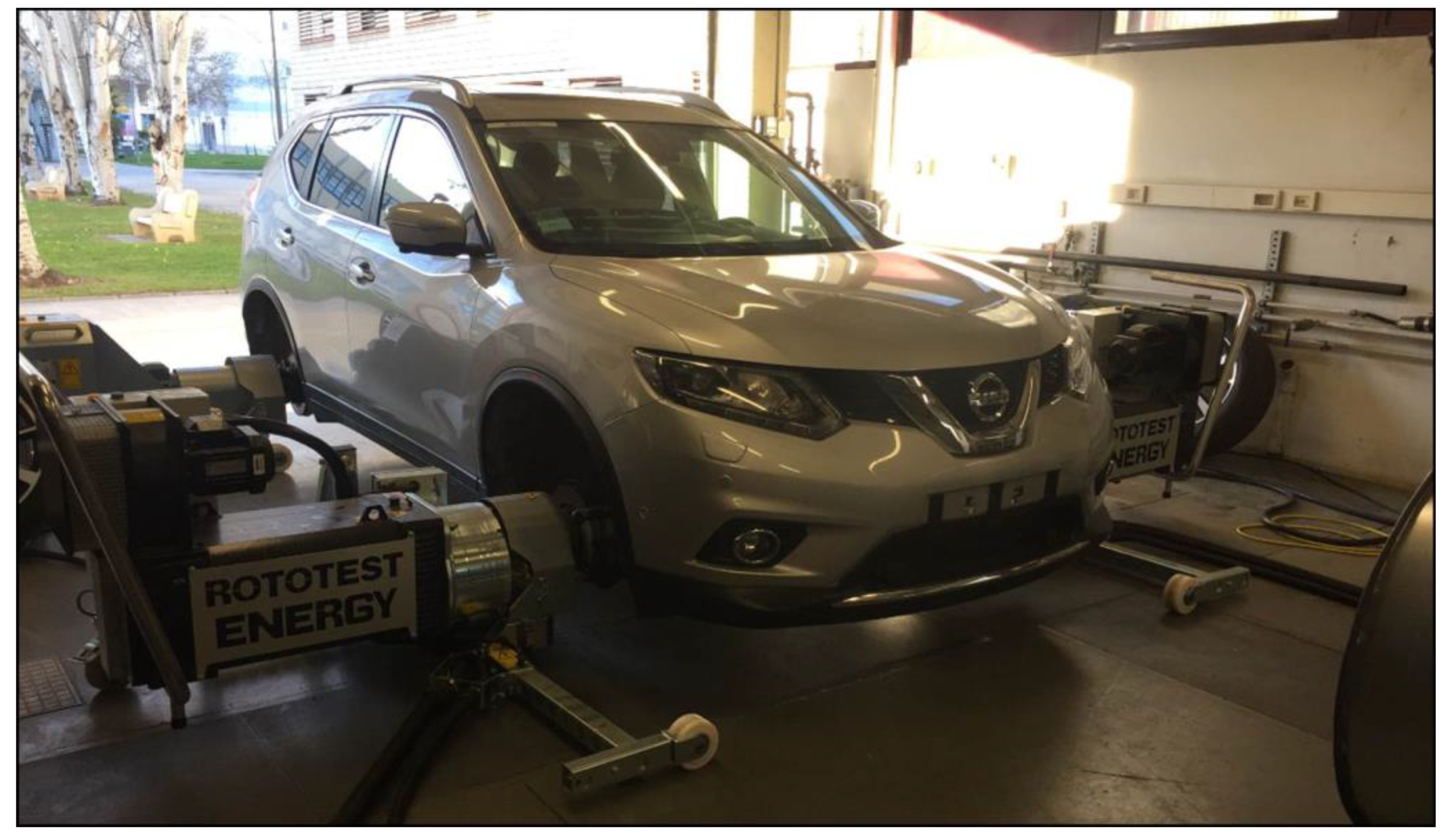
2.1. Vehicle

The vehicle (Figure 1) used in this study was a Nissan X-Trail with a 1.6 L, turbocharged, diesel engine equipped with high-pressure and low-pressure EGR. The engine provides a maximum power of 96 kW at 4000 rpm and a maximum torque of 320 Nm at 1750 rpm. The parameters provided by the ECU (Electronic Control Unit) of the vehicle were used for the analyses carried out.

Table 1. Vehicle specifications.

Parameter	Value
Mass	1575 kg
Drag coefficient	0.35
Frontal area	2.2 m2
Friction coefficient	0.015
Engine	Compression ignition, turbocharged
Displacement	1598 cm3
Max torque	320 Nm @ 1750 rpm
Max power	96 kW @ 4000 rpm

summarizes vehicle and engine characteristics.

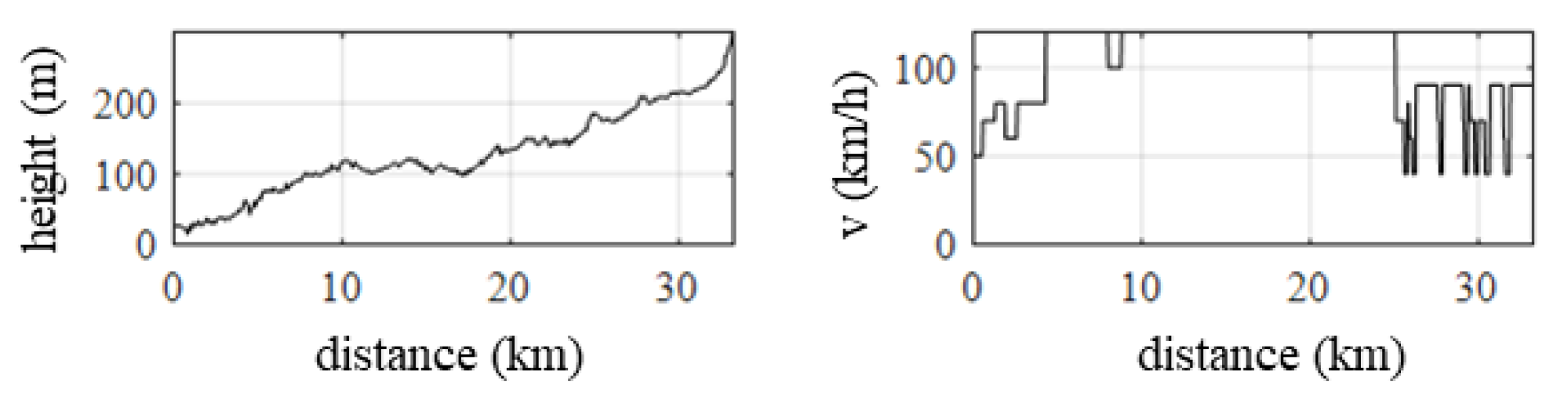
2.2. Route (Height and Speed Limits)

A route from Valencia city (approximately 0 m ASL) to Olocau town (approximately 300 m ASL) was chosen (see Figure 2). This route comprises an urban driving zone in a populated city and extra-urban driving until reaching the destination. The maximum speed during the route was 120 km/h. The total distance travelled was 33 km.

An initial driving test along the route to gather altitude and speed limit information was carried out. This data is shown in Figure 3.

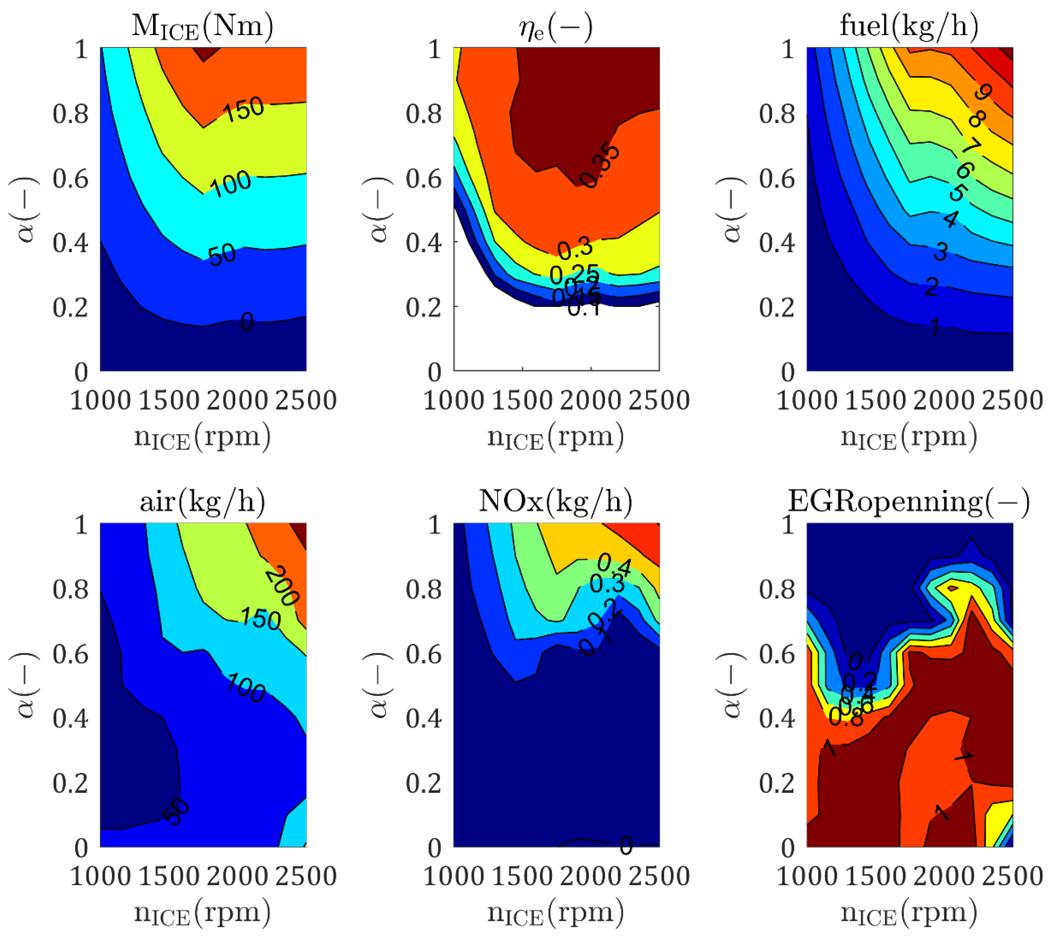
2.3. Engine Mapping

Bench tests were done to characterize the engine map. The tests were carried out maintaining a constant value of engine speed and the torque was increased to sweep the engine map (see Figure 4) The full load conditions were not reached, since they were not necessary to simulate the route.

2.4. Vehicle Modeling

In addition to the engine characterization, a vehicle model is needed to link the pseudo-stationary engine operating points to the driving conditions. A longitudinal dynamics approach was chosen for this work, while powertrain elements are modelled following the quasi-steady approach presented in [22,23].

The forces acting opposite to the movement of the vehicle are the aerodynamic drag, the road friction, the weight and, if we consider a non-inertial frame of reference, the inertia force.

The aerodynamic drag ($F_a$) is given by:

$$F_a=\frac{1}{2}\rho A{c}_d{v}^2$$

(1)

where $\rho$ is the air density, $A$ is the front area of the vehicle, $c_d$ the drag coefficient and $v$ the vehicle speed. Wind speed was not considered in the current study. The slope and weight contribution ($F_g$) is:

$$F_g=mg\sin \alpha$$

(2)

where $m$ is an equivalent vehicle weight, $g$ is the gravity acceleration and $\alpha$ is the road slope. For the friction force the following formulation was employed:

$$F_r=c_{r}mg \cos \alpha$$

(3)

where $c_r$ is the road friction coefficient, 0.015 in the case at hand. The inertia due to the mass of the vehicle is:

$$F_i=ma=m\dot{v}$$

(4)

where $a$ is the acceleration of the vehicle.

The last force against movement considered is the braking force:

$$F_b=u_b\widehat{F_b}$$

(5)

where $\widehat{F_b}$ is me maximum braking force and $u_b$ represents the brakes actuation: 0 corresponds to no braking and 1 to full braking.

The force that drives the vehicle forward is the force exerted by the wheels to the road:

$$F_t=\frac{T_w}{r_w}$$

(6)

where $T_w$ is the engine torque at the wheels provided by the powertrain and $r_w$ the radius of the wheel.

Applying Newton’s second law, the previous equations together result in the ordinary differential equation that describes the dynamics of the vehicle:

$$\dot{v}=\frac{F_{t }-F_a-F_r-F_g-F_b}{m}.$$

(7)

2.5. Optimization Problem

Considering a route defined by a distance to cover, the road height profile and speed limits depending on the vehicle position in the route, the target is to derive how a driver should behave to minimize a given cost index. In this work, optimal driving profiles have been calculated according to two different criteria: minimum fuel consumption and minimum Nox. The associated cost functions considered are, respectively:

$$J_{mf}=mi{n}_u \left\{{{\displaystyle \int }}_0^S\frac{{\dot{m}}_f\left(u\right)}{v\left(s\right)}ds\right\}$$

(8)

$$J_{NOx}=mi{n}_u \left\{{{\displaystyle \int }}_0^S\frac{{\dot{NO}}_x\left(u\right)}{v\left(s\right)}ds\right\}$$

(9)

where ${\dot{m}}_f$ and ${\dot{NO}}_x$ are respectively the fuel and NO_x mass flows to be minimized in a route of length S, $s$ is the vehicle position along the route, $v$ is the vehicle speed and $u$ is the driver decision, in the case at hand the throttle and brake positions. For the sake of simplicity, the gear has been chosen according to a predefined policy depending on the vehicle speed.

The optimization problem described in Equations (8) and (9) needs a regularization since the Nox and fuel consumption will be naturally reduced if more time is available to cover the route. In the limit, the fuel and Nox emissions will be null if the time to cover the route is infinity and the engine is not switched on. For the sake of regularization, the problem is constrained by imposing a limited route time ($\widehat{T}$ in Equation (3)):

$${{\displaystyle \int }}_0^S\frac{1}{v\left(s\right)}ds-\widehat{T}\le 0$$

(10)

An additional constraint is imposed due to the vehicle speed limitations in the route according as:

$$v\left(s\right)-\widehat{v}\left(s\right)\le 0$$

(11)

where $\widehat{v}\left(s\right)$ are the speed limitations.

The previously described optimization problem of finding the vehicle speed trajectories minimizing (8) or (9) while fulfilling constraints (10) and (11) and the equations describing the powertrain (1–7) fits perfectly in the Optimal Control framework [24].

Amongst the Optimal Control methods that can solve the proposed problem, Dynamic Programming is one of the more widespread algorithms due to its ability to provide a global optimum. Dynamic Programming is the numerical implementation of the Bellman’s Principle of Optimality [25], stating that “an optimal policy has the property that whatever the initial state and initial decisions are, the remaining decisions must constitute an optimal policy with regard to the state resulting from the first decisions”. Which essentially states that any sub-trajectory of an optimal trajectory must be also optimal between the initial and final states. In this sense, DP is based in discretizing the domain (in the case at hand the route length) in $n+1$ steps, the control and state spaces ($U$ and $X$) to evaluate the set of feasible trajectories between two consecutive steps and choose the optimal one. To perform a global optimization and consider the impact of current decisions on future state and cost evolution, the DP algorithm chooses at every step ($s_i$) the optimum cost-to-go function ($J_s^{*}$) defined as:

$$J_s^{*}\left(s_i\right)=\underset{u}{\min }\left\{L_s\left(X,U,s_i\right)+{\displaystyle \sum }_{k=i+1}^n{J}_s^{*}\left(s_k\right)\right\}$$

(12)

where $L_s\left(X,U,s_i\right)$ is the value of the cost function (in the case at hand fuel consumption or NOx emissions) in a single step depending on the combination of $U$ and $X$ in the current step $s_i$. In this sense, Equation (12) allows to transform an integral problem such as (8) or (9) in a sequence of single-step problems consisting in the selection of the minimum value of $J_s^{*}\left(s_i\right)$ from a finite set of candidates in a recursive way, starting from $s_n=S$ and proceeding backwards until $s_0=0$. A full description of the algorithm and its implementation can be found in Sundstrom and Guzzella [26].

Despite its ability to find a global optimum, DP suffers from the so-called curse of dimensionality, i.e., the number of combinations to evaluate rapidly rises as the number of controls, states and the problem length increases. So, in practice, the use of DP algorithms is usually limited to problems with low number of states and actuators. Considering the optimization problem described by Equations (8)–(11), one can identify 2 actuators, i.e., throttle and brake, since the gear is dependent on the vehicle speed, and one state, i.e., the vehicle speed that will be integrated according to Equation (7), while the vehicle speed limits, and road slope are considered disturbances a priori known. In addition, since efficient driving prevents from acting simultaneously on throttle and brake, both pedals can be modelled with a single variable, ranging from 1 (full throttle) to −1 (maximum braking effort), then leading to a 1 state (vehicle speed), 1 actuator (throttle-brake) optimization problem that can be handled by DP algorithm.

3. Results

Following the methods described in the previous section, the engine map with the pseudo-stationary operating modes and two driving profiles (minimum fuel consumption and minimum NOx emissions) were obtained.

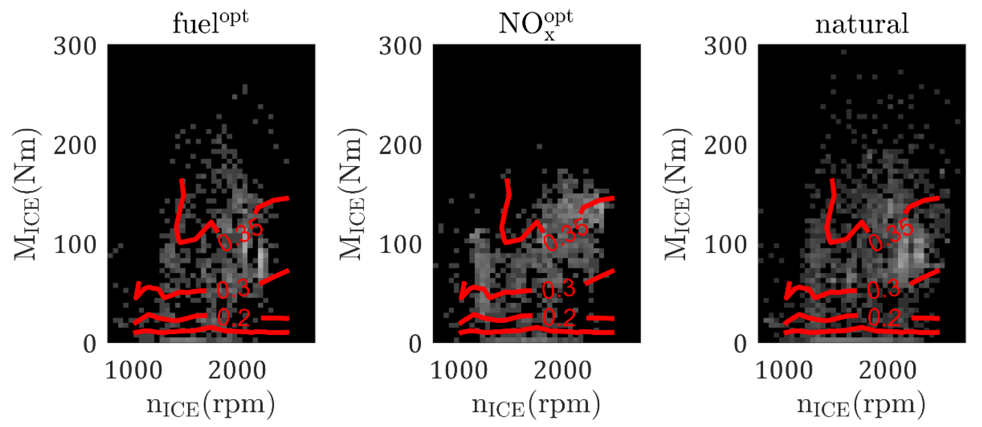
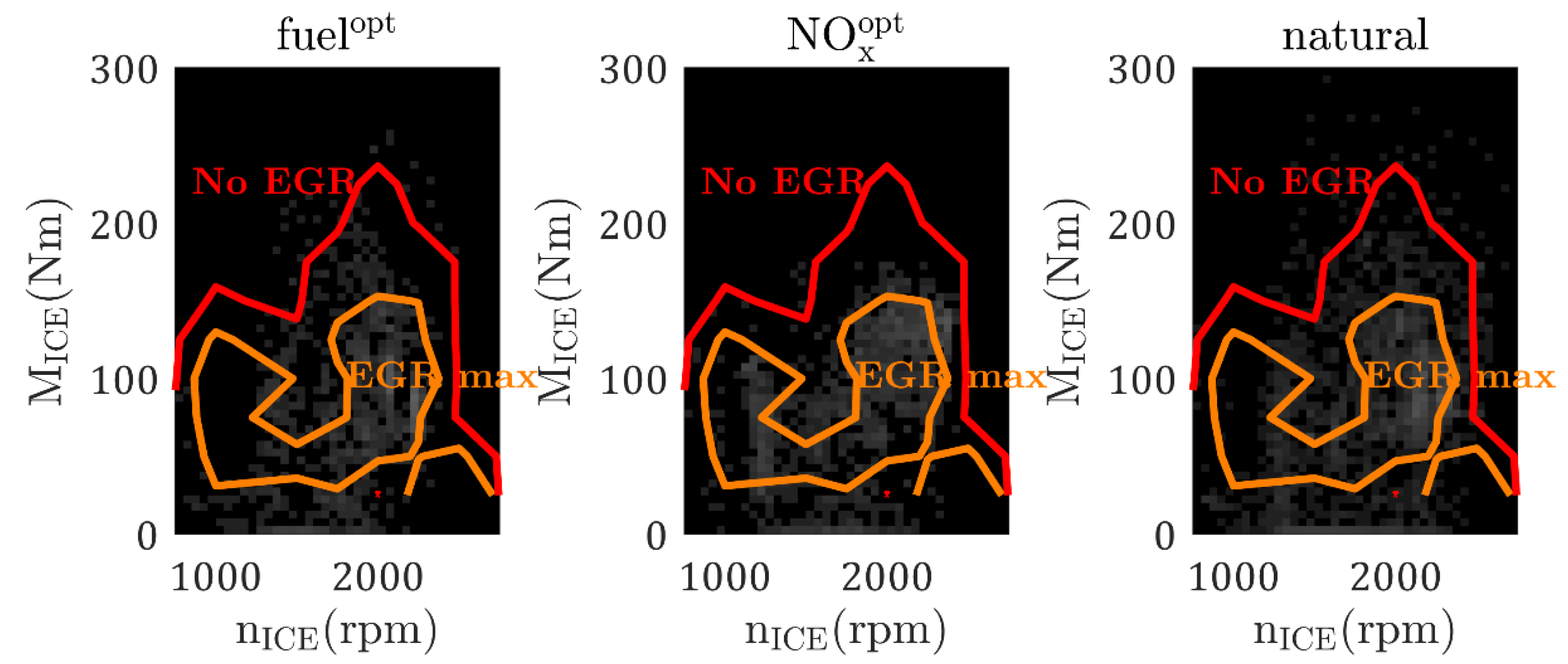
3.1. Engine Maps

From the bench tests, engine maps of the relevant parameters were obtained as a function of throttle position and engine speed (see Figure 5). Results show how the engine can reach peak efficiencies clearly above 35% in a wide area of medium engine speeds and medium to high loads. However, this high efficiency is reached, amongst other reasons, due to a limited EGR rate. In fact, as the EGR valve opening map shows, there is not exhaust gas recirculation in the high load area. Then, in those conditions the engine operates with high efficiency, but also with high NOx emissions. Note the clear correlation between the area of high NOx emissions and the area without EGR. The differences between the engine operating conditions areas for minimum NOx emissions and maximum engine efficiency, lead to predict that the optimal vehicle speed profile for NOx minimization will be noticeably different to that for fuel consumption optimization.

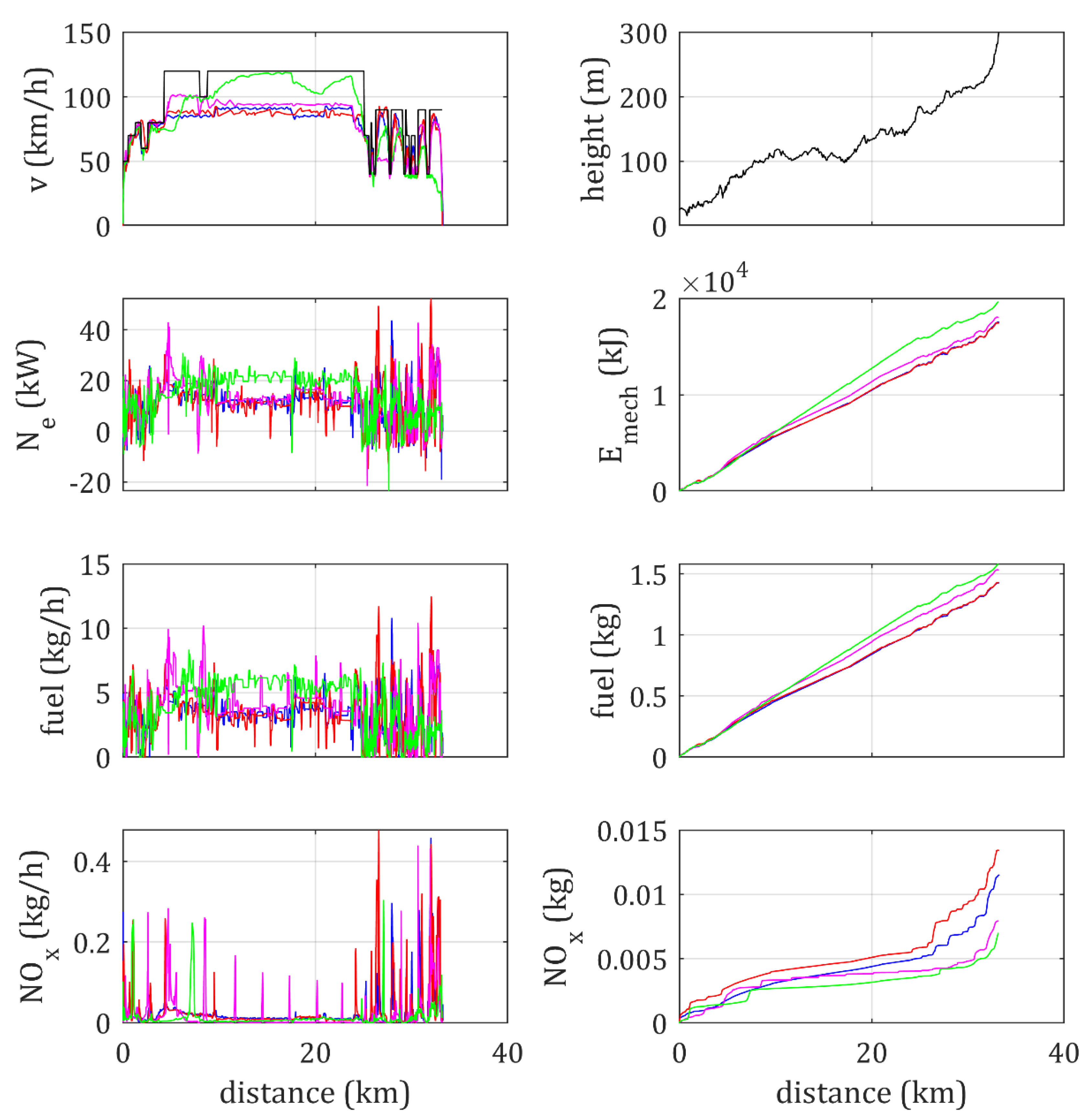
3.2. Optimal Driving Profile and Deviations for the Implemented Optimal Speed Profile

The optimal profiles were implemented in a test cycle on a bench test with the vehicle. The main difficulty in the implementation was to follow the calculated speed profiles at low vehicle speeds and gear ratios due to dyno inertia issues and driver capabilities. Figure 6 shows the calculated and the driving profile measured in the tests and the distribution of the error between the demanded and measured vehicle speed. It can be observed how deviations between measured and desired vehicle speed at low velocities (and high accelerations) can exceed ± 5 km/h, while as speed increases this error is reduced and at high vehicle speeds and gears was easier to follow the driving profile (±1 km/h).

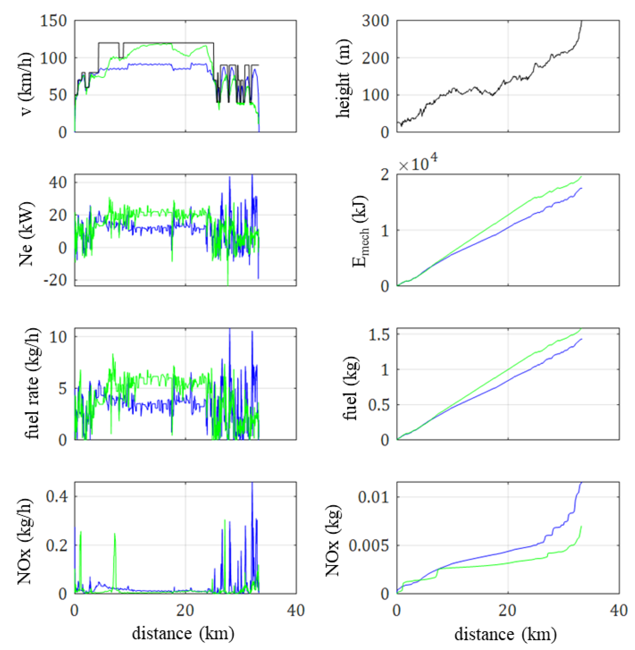
3.3. Optimal Driving for Reduction in Fuel Consumption and NOx

The optimal driving profiles for reduction in fuel consumption (in blue) and NOx (in green) are shown in Figure 7. As it can be seen, the driving profile for maximum fuel efficiency (blue) tends to maintain a constant speed were possible and its maximum speed is around 90 km/h. Meanwhile, the driving profile for minimum NOx reaches the maximum speed limit of 120 km/h and has lower accelerations.

The optimal driving profile for fuel economy approaches the speed limits in both urban and rural segments while stays at relatively low vehicle speeds in comparison with the limit in highway conditions. Particularly, in highway driving where the speed limit is 120 km/h, the maximum speed does not exceed 90 km/h to avoid the increase in energy losses at higher speeds, particularly the aerodynamic drag force, which is proportional to the squared speed (Equation (1)). The NOx emissions with the fuel minimization strategy present peaks due to fast accelerations commanded by the optimization strategy, especially at the last phase of the cycle when speed limits change abruptly with high frequency.

The driving profile for NOx reductions shows a smoother variation in the vehicle velocity and higher values, approaching the limit of 120 km/h in the highway driving. The optimization algorithm tends to increase the vehicle speed at the highway area, where the road slope is low, to save time and allow lower vehicle speeds in the last part of the cycle where high load demands due to the road slope will make the engine work outside of the EGR area (see Figure 5) and then produce NOx. Note that due to this fact, in the last part of the cycle the NOx oriented strategy strongly improves the NOx emission results obtained with the fuel minimization strategy. Of course, the improvement in NOx emissions is done at the expense of an increase in fuel consumption as shown in the plots in the third row of Figure 7.

Part of the penalty in fuel consumption of the NOx oriented strategy may be due to the operation of the engine in the EGR zone, then with lower efficiency, but the results on the effective power of the engine and the associated cumulated mechanical energy (see second row of Figure 7) show that most of the fuel saving with the optimum fuel consumption strategy is due to the fact that the vehicle requires less energy to drive according to its speed profile. The reduction in the maximum vehicle speed in the highway area leads to an almost constant fuel saving between kilometers 6 and 27, and despite in the last part of the cycle (rural area), the lower speed of the NOx oriented strategy allows to recover part of the fuel consumption, the fuel-oriented strategy produces an improvement in fuel consumption of 10%.

To validate the driving strategies obtained, they were compared with two additional arbitrary driving profiles (see Figure 8, in red). These profiles, although arbitrary, followed the same restrictions as the optimal driving ones and, since they were registered without following any vehicle speed profile, they are assumed to be representative of natural driving.

It can be observed that the speed profiles for natural driving shown in Figure 8 are more similar to the optimal fuel consumption profile than to the optimal NOx profile. The intuitive reason is that if a driver wants to cover a route in a given time, he will naturally tend to keep an almost constant speed near the average speed. In this sense, one of the driving cycles with natural driving shows a negligible fuel consumption penalty of 0.05%. The other natural driving cycle, with a substantially higher vehicle speed between kilometers 5 and 8 shows a penalty in fuel consumption of 7.5%.

Regarding NOx, both natural driving cycles show important penalties in front of the optimal NOx driving profile.

Figure 9 shows a summary of the fuel consumption and NOx emissions obtained in the tested driving cycles. Results show that (see Figure 9), in terms fuel consumption, a 10% reduction was obtained for the minimum fuel consumption driving profile with respect to the minimum NOx profile. The two arbitrary driving profiles (in red) were better in terms of fuel consumption than the minimum NOx profile, but still show a penalty of 4% in fuel consumption respect to the fuel optimal driving cycle.

Regarding the NOx production, the optimal driving profile (green) was found to reduce a 38% the NOx emissions compared to the driving profile for minimum fuel consumption. Both arbitrary driving profiles (red) were above the NOx levels of the optimal driving profile with an average penalty of 34.5% in NOx emissions.

One can see that differences in terms of NOx emissions tend to be higher due to the exponential growth on NOx emissions with engine load shown in Figure 5. In this sense, the driving profile has an even higher impact on NOx emissions than in fuel consumption and accordingly it becomes a key factor to limit the environmental impact of actual driving.

While Figure 7, Figure 8 and Figure 9 provide the evolution and the summary of the key vehicle operating variables and performance indexes, the justification of the difference in the results requires the analysis of the engine operating conditions. To this aim, Figure 10 shows the probability distribution of the engine operating conditions in the engine efficiency map. One can clearly see that the operating conditions in the natural driving span a wider area of the engine map, while following a defined driving cycle such as those for minimum fuel consumption, and especially minimum NOx emissions restrict the range of operating conditions. One can also see a high frequency operating area around 2100 rpm and 100 Nm for the minimum fuel and natural driving cycles due to the almost constant vehicle speed at highway conditions. On the contrary, this area of high probability is not observed for the case of the minimum NOx driving cycle. Regarding efficiency, it cannot be observed that the minimum fuel driving cycle operates more frequently in a high efficiency area, so the main part of the fuel saving with this cycle cannot be associated with a higher engine efficiency, but from a minimization of the external loads.

To justify the differences in NOx emissions, Figure 11 shows the probability distribution of the engine operating conditions in the EGR opening map. It can be clearly observed how most of the operating points in the optimum NOx emissions cycle are placed in the area of maximum EGR opening and the engine barely operates outside of the EGR region. The driving cycle for fuel minimization spans the operating conditions to the area of low EGR opening (engine speed between 1500 and 2000 rpm and torque above 140 Nm) and sporadically exits the EGR area. Finally, in natural driving, where the driver does not follow any prescribed speed profile, the engine frequently operates in the low EGR opening area and even in conditions without EGR. Due to this reason, strong differences in terms of NOx emissions shown in Figure 9 are justified.

Finally, Figure 12 represents the cumulative distribution observed for the engine effective power (as a measure of the mechanical power needed to drive the vehicle), the engine efficiency and the NOx emissions. The distribution of the engine effective power clearly shows how the speed profile for fuel consumption minimization clearly shows lower mechanical power requirements, that at the end of the day lead to noticeable fuel consumption savings. As the vehicle speed profile obtained with natural driving is like the one for fuel consumption minimization, the distribution in mechanical energy is also similar. An exception is the area of high-power demands (above 25 kW) which is clearly more frequent with natural driving due to the arbitrary accelerations appearing in those cycles. On the contrary, the high vehicle speed required in highway driving by the minimum NOx driving cycle led to a mechanical power distribution displaced to the right in the range of 15–25 kW. However, one can see that mechanical power demands above 25 kW are barely achieved with the NOx oriented strategy since the vehicle speed in the rural area (with high slope and frequent changes in the vehicle speed limit) is kept low to avoid NOx.

Regarding the engine efficiency distribution, results in the central plot of Figure 12 do not show significant differences amongst driving cycles, pointing out that the fuel saving achieved with the fuel optimal driving cycle relies mostly on the savings in the required mechanical energy. This is an important result since gives insight on the fact that, if the objective is to minimize the fuel consumption, an optimization focused on reducing the required mechanical energy, then without including the engine response, will provide fairly good results. Note the interest of this simplification, since obtaining data on the main vehicle dynamics is easy in comparison with obtaining results to model the engine behavior, that need an experimental facility and the corresponding instrumentation.

Finally, the distribution in the NOx emission shows the important benefits of the NOx oriented strategy that maximizes the engine operation with EGR as shown in Figure 11.

4. Conclusions

Using dynamic programming, two driving profiles for two different objectives were obtained: minimizing fuel consumption and minimizing NOx emissions. The vehicle model consisted of longitudinal dynamics that link road driving conditions to pseudo-stationary modes tested in bench. From the results following conclusions can be drawn:

• The results show high potential for advanced driver-assistance systems in fuel consumption and especially in emissions reduction. In this sense, there is a substantial potential of fuel consumption and emission reduction in adapting the speed profile to the driving conditions (road slope, speed limits, time constraints or traffic).
• The common approach of optimal driving for fuel economy it is not the optimal for NOx pollutant emissions. NOx should be considered when optimizing fuel consumption.
• The fuel optimal driving profile obtained a 4% reduction in fuel consumption with respect to the NOx reduction driving profile.
• Most of the fuel saving potential is obtained by means of the mechanical energy minimization, so even without information on the engine, substantial fuel savings can be obtained by speed profile optimization.
• Natural and smooth driving, i.e., keeping vehicle speed as constant as possible approaches the minimum fuel consumption profile while more complex speed profiles are required for reducing NOx emissions.
• The NOx reduction driving profile was found to reduce 34.5% NOx emissions compared to the driving profile for minimum fuel consumption. In this sense, considering emission criteria in algorithms for driver assistance is a key point to reduce vehicle environmental impact.

5. Future Works

A further analysis with more engine parameters and with different fuels and their impact in driving profiles is to be achieved.

References

- García-Contreras, R.; Gómez, A.; Fernández-Yáñez, P.; Armas, O. Estimation of thermal loads in a climatic chamber for vehicle testing. Transp. Res. Part D Transp. Environ. 2018, 65, 761–771. [Google Scholar] [CrossRef]
- Fernández-Yáñez, P.; Armas, O.; Martínez-Martínez, S. Impact of relative position vehicle-wind blower in a roller test bench under climatic chamber. Appl. Therm. Eng. 2016, 106, 266–274. [Google Scholar] [CrossRef]
- García-Contreras, R.; Soriano, J.A.; Fernández-Yáñez, P.; Sánchez-Rodríguez, L.; Mata, C.; Gómez, A.; Armas, O.; Cárdenas, M.D. Impact of regulated pollutant emissions of Euro 6d-Temp light-duty diesel vehicles under real driving conditions. J. Clean. Prod. 2021, 286, 124927. [Google Scholar] [CrossRef]
- Gómez, A.; Fernández-Yáñez, P.; Soriano, J.A.; Sánchez-Rodríguez, L.; Mata, C.; García-Contreras, R.; Armas, O.; Cárdenas, M.D. Comparison of real driving emissions from Euro VI buses with diesel and compressed natural gas fuels. Fuel 2021, 289, 119836. [Google Scholar] [CrossRef]
- Godiganur, V.S.; Nayaka, S.; Kumar, G.N. Thermal barrier coating for diesel engine application—A review. Mater. Today Proc. 2020, 45, 133–137. [Google Scholar] [CrossRef]
- Ezzitouni, S.; Fernández-Yáñez, P.; Sánchez, L.; Armas, O. Global energy balance in a diesel engine with a thermoelectric generator. Appl. Energy 2020, 269, 115139. [Google Scholar] [CrossRef]
- García-Contreras, R.; Agudelo, A.; Gómez, A.; Fernández-Yáñez, P.; Armas, O.; Ramos, Á. Thermoelectric Energy Recovery in a Light-Duty Diesel Vehicle under Real-World Driving Conditions at Different Altitudes with Diesel, Biodiesel and GTL Fuels. Energies 2019, 12, 1105. [Google Scholar] [CrossRef] [Green Version]
- Fernández-Yáñez, P.; Gómez, A.; García-Contreras, R.; Armas, O. Evaluating thermoelectric modules in diesel exhaust systems: Potential under urban and extra-urban driving conditions. J. Clean. Prod. 2018, 182, 1070–1079. [Google Scholar] [CrossRef]
- Boodaghi, H.; Etghani, M.M.; Sedighi, K. Performance analysis of a dual-loop bottoming organic Rankine cycle (ORC) for waste heat recovery of a heavy-duty diesel engine, Part I: Thermodynamic analysis. Energy Convers. Manag. 2021, 214, 113830. [Google Scholar] [CrossRef]
- Baldasso, E.; Mondejar, M.E.; Andreasen, J.G.; Rønnenfelt, K.A.T.; Nielsen, B.Ø.; Haglind, F. Design of organic Rankine cycle power systems for maritime applications accounting for engine backpressure effects. Appl. Therm. Eng. 2020, 178, 115527. [Google Scholar] [CrossRef]
- Hu, J.; Li, J.; Hu, Z.; Xu, L.; Ouyang, M. Power distribution strategy of a dual-engine system for heavy-duty hybrid electric vehicles using dynamic programming. Energy 2021, 215, 118851. [Google Scholar] [CrossRef]
- Sher, F.; Chen, S.; Raza, A.; Rasheed, T.; Razmkhah, O.; Rashid, T.; Rafi-ul-Shan, P.M.; Erten, B. Novel strategies to reduce engine emissions and improve energy efficiency in hybrid vehicles. Clean. Eng. Technol. 2021, 2, 100074. [Google Scholar] [CrossRef]
- Donkers, A.; Yang, D.; Viktorović, M. Influence of driving style, infrastructure, weather and traffic on electric vehicle performance. Transp. Res. Part D Transp. Environ. 2020, 88, 102569. [Google Scholar] [CrossRef]
- Asadi, B.; Vahidi, A. Predictive Cruise Control: Utilizing Upcoming Traffic Signal Information for Improving Fuel Economy and Reducing Trip Time. IEEE Trans. Control Syst. Technol. 2011, 19, 707–714. [Google Scholar] [CrossRef]
- Wadud, Z.; MacKenzie, D.; Leiby, P. Help or hindrance? The travel, energy and carbon impacts of highly automated vehicles. Transp. Res. Part A Policy Pract. 2016, 86, 1–18. [Google Scholar] [CrossRef] [Green Version]
- Zavalko, A. Applying energy approach in the evaluation of eco-driving skill and eco-driving training of truck drivers. Transp. Res. Part D Transp. Environ. 2018, 62, 672–684. [Google Scholar] [CrossRef]
- Barth, M.; Boriboonsomsin, K. Energy and emissions impacts of a freeway-based dynamic eco-driving system. Transp. Res. Part D Transp. Environ. 2009, 14, 400–410. [Google Scholar] [CrossRef]
- Mensing, F.; Trigui, R.; Bideaux, E. Vehicle trajectory optimization for application in ECO-driving. In Proceedings of the 2011 IEEE Vehicle Power and Propulsion Conference, Chicago, IL, USA, 6–9 September 2011; pp. 1–6. [Google Scholar]
- Mensing, F.; Trigui, R.; Bideaux, E. Vehicle trajectory optimization for hybrid vehicles taking into account battery state-of-charge. In Proceedings of the 2012 IEEE Vehicle Power and Propulsion Conference, Seoul, Korea, 9–12 October 2012; pp. 950–955. [Google Scholar]
- Wegener, M.; Koch, L.; Eisenbarth, M.; Andert, J. Automated eco-driving in urban scenarios using deep reinforcement learning. Transp. Res. Part C Emerg. Technol. 2021, 126, 102967. [Google Scholar] [CrossRef]
- Hellström, E.; Åslund, J.; Nielsen, L. Design of an efficient algorithm for fuel-optimal look-ahead control. Control Eng. Pract. 2010, 18, 1318–1327. [Google Scholar] [CrossRef] [Green Version]
- Rizzoni, G.; Guzzella, L.; Baumann, B.M. Unified modeling of hybrid electric vehicle drivetrains. IEEE/ASME Trans. Mechatron. 1999, 4, 246–257. [Google Scholar] [CrossRef]
- Guzzella, L.; Sciarretta, A. Vehicle Propulsion Systems: Introduction to Modeling and Optimization, 3rd ed.; Springer: Berlin/Heidelberg, Germany, 2013. [Google Scholar]
- Bryson, A.E.; Ho, Y.-C. Applied Optimal Control: Optimization, Estimation, and Control; Routledge: Boca Raton, FL, USA, 2017. [Google Scholar]
- Bellman, R. The theory of dynamic programming. Bull. Amer. Math. Soc. 1954, 60, 503–515. [Google Scholar] [CrossRef] [Green Version]
- Sundstrom, O.; Guzzella, L. A generic dynamic programming Matlab function. In Proceedings of the 2009 IEEE Control Applications (CCA), Intelligent Control (ISIC), St. Petersburg, Russia, 8–10 July 2009; pp. 1625–1630. [Google Scholar]