Improving the Load Estimation Process in the Design of Rural Electrification Systems ^†

Abstract

The design of reliable and sustainable rural electrification systems relies on accurate prediction of the electrical load. This paper evaluates the current methods for load estimation and proposes an improved approach for load estimation for off-grid unelectrified rural communities that yields more accurate estimates. Improved accuracy is mainly due to better modelling of the influence of customer habits and gender on the estimated current and future load using the Markov chain process. A program was developed using MATLAB software to generate load profiles. The results show that gender considerations have a significant impact on load profiles and that the Markov chain process can suitably be used to determine year-to-year load profiles by incorporating the effect of changes in customer habits on the estimated load. The results from the case study on energy consumption in rural community households showed an increase in average daily consumption when gender was considered during load estimation. The peak consumption when gender was considered was about 50% higher than the value for when gender was not considered.

1. Introduction

Load modelling or estimation is a critical step in the design of rural electrification systems such as those that utilize solar photovoltaics (PV). Load modelling enables the creation of load profiles that indicate the consumption of electricity over a given time period usually over a full day. The energy consumption is the amount of energy in Watthours (Wh) required by the particular users in a given day [1]. Poor load estimation leads to undersize or oversize of the system. This issue, in turn, results in a less reliable or more expensive system. During load estimation, the community’s electric needs are grouped into categories that have similarity in electricity usage [2]. The common categories in rural areas include households, shops, restaurants, milling, welding, churches, mosques, and healthcare centres. The energy consumption for these categories depends on the appliance ratings, the community activities and the people’s way of life [1]. This consumption varies with the day of the week and season of the year. Estimating the load profile for rural communities in developing countries is quite challenging. This, among other reasons, is due to the scarcity of information on electricity consumption in rural communities since a majority of the people in those communities do not have access to electricity. The electricity consumption in rural communities is generally limited to minimal uses such as lighting, phone charging and use of small radios [3].

Numerous studies such as those presented in [1,4,5] have been undertaken on load estimation for rural electrification. Studies such as [6,7,8,9,10] have used simple equations to estimate the daily load based on the appliance power ratings and duration of use. The equations can be scripted in available tools such as Microsoft Excel to further ease computation and replication of the procedure to various locations [11,12]. Mandelli [1] and Mandelli [4] used stochastic bottom-up that correlates between load factor and coincidence factor to build up the coincidence behaviour of the electrical appliances considered by the users. Their approach provides a way of building hourly load consumption profiles for rural communities that do not have electricity. The resultant load profiles take into consideration the uncertainty of the load in rural communities. Blodgett [5] discussed the shortcomings of using questionnaires in determining the community’s electricity needs. Their rationale was to reduce inaccuracy in load estimation caused by the use of questionnaires when determining electricity needs. Their study showed that these shortcomings could be overcome by using a microgrid of one community to estimate the consumption of another. The above studies do not explain the effect of socio-economic characteristics on the load profile of off-grid rural communities.

This paper is an elaboration of the work we presented in [13]. It gives a more detailed explanation of the entire proposed load estimation approach than was presented in [13], which focused mainly on detailing the gender considerations in load estimation. The key contributions of this study are:

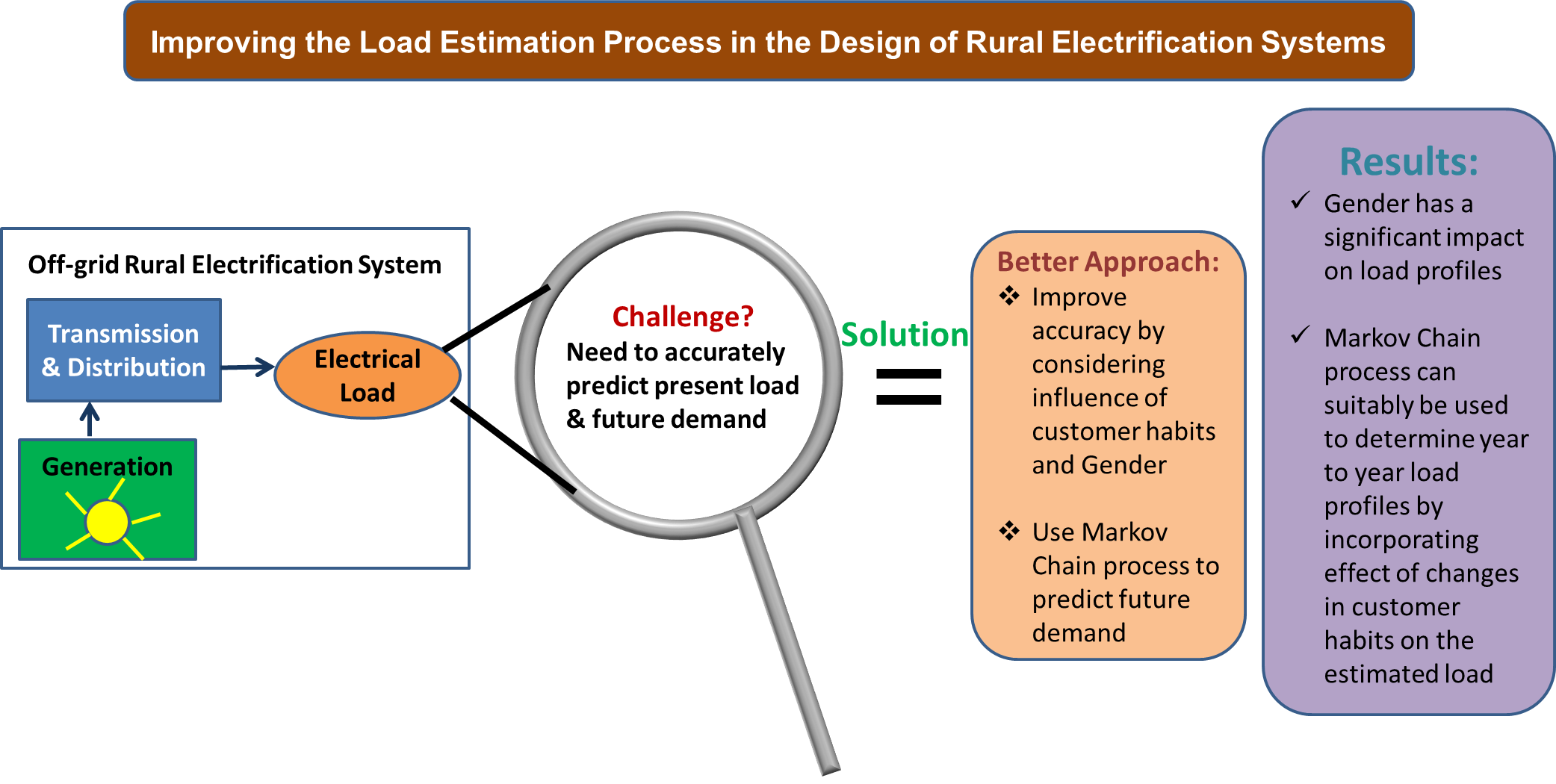
• It proposes a load estimation methodology for off-grid rural electrification systems that incorporates socio-economic characteristics of an area.
• It highlights the effect of gender on load profiles.
• It shows how Markov chain process can be used in the design of year-to-year load profiles for off-grid unelectrified rural communities.
• It presents a much simpler approach to load modelling and is still based on the bottom-up approach.

The rest of the paper is organized as follows: Section 2 provides a review of the current methods for electricity load profile generation; Section 3 presents the improved approach to load estimation for off-grid systems proposed in this study; Section 4 provides an illustration of this proposed load estimation approach and the results obtained; and lastly, Section 5 provides the conclusions drawn from this study.

2. A Review of Current Approaches for Electricity Load Profile Models

In order to effectively evaluate the existing methods for load estimation, characteristics of an exemplary load profile have been defined [3,14,15]. As stated in [13], these include:

• It is parametric, thus able to simulate various scenarios of energy consumption [15].
• The specificities of the load categories (such as households, small and large business enterprises) and equipment must have a contribution towards the load profile results [15].
• The socio-economic conditions and the daily behaviours of the rural community must have a contribution to the load profile [3,5].
• It has to be stochastic to embrace the uncertainty of energy consumption [3].
• It must be aggregative, allowing profiles to be generated by summing up multiple profiles for different categories of the community (such as households and schools) [15].

A review of the current methods that have been used to analyse load profiles in rural areas may be summarised as follows:

i.

For some methods, the researchers do not provide any explanation on how the load profile was developed. There is, therefore, no chance to evaluate whether the researcher undersized or oversized a profile. In addition, they do not take into consideration the socio-economic behaviours [1,4,16].

ii.

For some methods, the appliances, power ratings, and time windows within which an appliance may be switched on are determined. The hourly power consumption of each appliance is determined by assuming that all appliances are on at the same time in a precisely defined window. This method overestimates the peak usage and does not also take into consideration the socio-economic behaviours [1,4].

iii.

The appliances, power ratings, and time windows within which an appliance may be switched on are determined. In addition, the actual time in hours for which the appliance is switched on is determined after which the power consumption is determined. The resultant power is distributed equally over the time windows for which the appliance may be active. This method produces a peak power that is most likely less than the actual peak and does not take into consideration the socio-economic behaviours [1,4].

iv.

The load profiles are assumed to be similar to those in communities of similar contexts [4,17]. The research however does not provide an explanation as to how their characteristics are compared and does not embrace the uncertainty of energy consumption in the rural areas.

v.

In another method, the users’ electric needs are categorized into user classes, electric appliances and usage habits. This categorization includes appliances, power ratings, and time windows within which an appliance may be switched on and actual hours in a day that an appliance is on. The hourly appliance usages are aggregated into a load profile. Random variables are introduced to simulate the likelihood of appliance usage throughout the day, and reasonable estimations of the load profiles are obtained [3,5,17,18].

The approach described in (v) provides more accuracy than the approaches described in (i) to (iii) and can simulate various stochastic scenarios of energy consumption [4,5,19,20,21]. However, the accuracy may be affected by inaccurate predictions of the current and anticipated appliance inventory, power ratings, and times of use and also the approach does not consider changes in load depending on anticipated changes in the welfare and habits of the communities [5,22].

This evaluation shows that there is still a need for a load estimation approach that incorporates socio-economic and gender aspects. As thoroughly discussed in [13], gender roles within the community significantly affect the choice of appliances and time of use both in the households and community projects. Ignoring gender aspects may lead to inaccurate estimation of the load, which in turn leads to either oversize or undersize of the system. Some of the gender considerations include:

• A gendered approach to identifying the electric needs of the community;
• Financial decision making in the household;
• Asset ownership and control of assets;
• Gender distribution of roles in the management of community-based projects;
• Cultural constraints.

3. Proposed Improved Load Modelling Approach

In this study, an improvement in the stochastic method to simulate load characteristics that change with change in customer habits and community conditions is proposed. This improved approach incorporates gender aspects in the load estimation. It also uses average consumption in a similar village that is already electrified as a measure of the consumption in the unelectrified village and adjusts the load profiles accordingly to fit the socio-economic setup of the new village as shown in Figure 1. The first step of this approach is to identify an electrified village whose setup and social characteristics are similar to that of the village to be electrified. After identifying the village, the following procedure is used to determine the load of the unelectrified village.

(a)

Carry out a survey in the electrified village.

The appliances, ratings and usage times for the electrified village are identified. In addition, the monthly electricity bill for each customer is obtained. The average daily usage of each customer is estimated from their monthly bills. The users are categorized according to their electricity needs. The common categories in rural areas include households, shops, restaurants, milling, welding, churches, mosques, and healthcare centres. The sample customers in the survey should include all the customer types that are homes and businesses. Households account for a significant part of the electrical load and electricity consumption varies a lot among households than the other customer categories [23]. During the survey, the following parameters are used to classify the households.

(i)

Average household size.

(ii)

The education level of the household head.

(iii)

Economic activities of the household head.

(iv)

Gender of the household head.

(v)

The age range of the household head.

(vi)

Type of house. The common dwelling types include the following [24]:

• Brick house with irons sheets roof, more than two rooms, kitchen, toilet, lounge;
• Brick house with iron sheets roof, two sleeping rooms, kitchen, toilet, lounge;
• Brick house with iron sheets roof, one sleeping room, kitchen, toilet, lounge;
• Brick house with grass roof, more than two sleeping rooms, kitchen, toilet, lounge;
• Brick house with grass roof, two sleeping rooms, kitchen, toilet, lounge;
• Brick house with grass roof, one sleeping room, kitchen, toilet, lounge;
• Mud-house with grass, more than one sleeping room, kitchen, toilet, lounge;
• Mud-house with grass, one sleeping room, kitchen, toilet, lounge.

The hourly consumption throughout the year is determined, as discussed in Section 3.1. The customers are classified as High, Medium, or Low depending on their consumption. The socio-economic and gender-related characteristics of the electrified village are evaluated. The customers are categorized according to their willingness and ability to pay for the electricity. Details of customer transition among categories of consumption and ability to pay are determined as discussed in Section 3.2.

(b)

Carry out a survey in the unelectrified village.

The customers in the unelectrified village are classified according to their electricity needs. Each customer is assigned a daily load based on the consumption of a similar customer in the electrified village. The change in load consumption over time is estimated using:

• The differences in the socio-economic and gender characteristics of the two villages and changes in electricity consumption;
• The ability to pay identified in the electrified village.

(c)

Determine the load profile for the unelectrified village.

The number of customers to be connected to the microgrid is determined. The load profile of the microgrid is also determined.

If it is not possible to identify a proxy village or identify a specific customer category in the electrified village, then an energy survey is carried out in the unelectrified village. The following is determined: the appliances, ratings, and usage times are estimated. The hourly consumption throughout the year is determined, as discussed in Section 3.1. The customers are classified as High, Medium, or Low depending on their electricity consumption. The socio-economic and gender-related characteristics of the customers are evaluated. The customers are categorized according to their willingness and ability to pay for electricity services. Details of customer transition among categories are determined. The change in load consumption and customer’s ability to pay over time is estimated. The number of customers to be connected and the load profile of the microgrid are determined. Since there is no proxy village, there is no pre-defined range for the average daily consumption of the consumers. Therefore, the results may be over or under-estimated due to inaccuracies in the number of the present and anticipated appliance ownership, appliance ratings, and time of use.

3.1. Energy Survey in Electrified Village

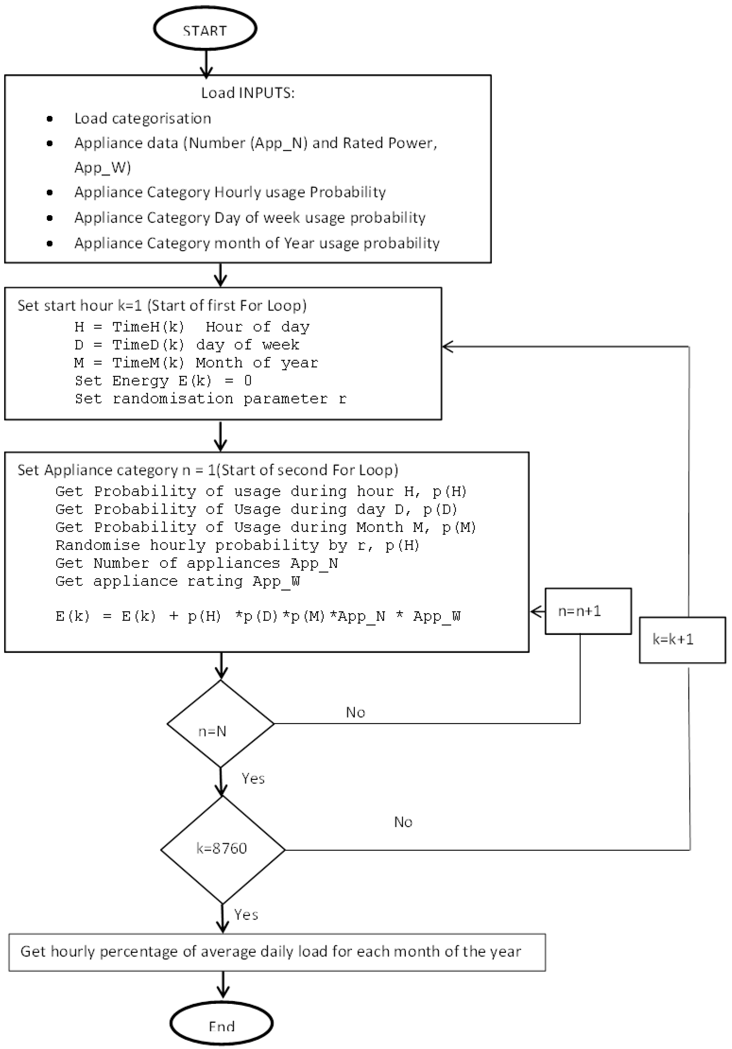
Steps for Determining the Load Profile

(i)

Determine the load consumption per hour for each appliance.

According to [20], the load for a given appliance at time t is given by Equation (1).

$$E_t=\frac{N}{n}{\displaystyle \sum }{P}_t \left(1\right)$$

(1)

where n is the total number of appliances owned by the interviewed sample customers, and N is the total number of appliances in a given category. $P_t$ is the power rating of the appliance.

Equation (1) may be reformulated as (2).

$$E_t=N\ast \frac{number of appliances switched on at time t\ast P_t }{n}$$

(2)

However, the probability that an appliance in the sample is switched on at time t is given by

$$Probability at time t=\frac{number of appliances switched on at time t}{n}$$

(3)

Therefore, the energy at time t is given by (4).

$$E_t=N\ast Probability at time t \ast P_t$$

(4)

In situations where few observations can be made about the collected data from interviews, the probability is estimated using (5) [20].

$$Probability at time t=\frac{hours appliance is on during a period}{Total hours in period}$$

(5)

(ii)

Define load characteristics depending on socio-economic activities of the area.

As mentioned before, the socio-economic conditions and daily behaviours of the community must have a contribution to the load profile. Research carried out in [23,25] and [26] shows that the probability that an appliance is switched on varies by the hour, day of the week, and month. Equation (4) has, therefore, been modified to (6).

$$E_t=N\ast P_{th}\ast P_{td} \ast P_{tm}\ast P_t$$

(6)

where $P_{th}$ is the probability that an appliance in a category is switched on at a given hour, $P_{td}$ is the probability that an appliance in a category is switched on, on a given day, $P_{tm}$ is the probability that an appliance in a category is switched on in a given month, and $P_t$ is the appliance power rating.

(iii)

Randomize the number of appliances switched on per hour.

A good load model should be stochastic in nature. From step (i), the probability that an appliance is on has been defined. It indicates the number of appliances switched on simultaneously at a given time. The unpredictability in appliances switching on and off needs to be catered for. The number of appliances may be assumed to vary randomly in the range of ±a% of the mean. Varying the number of appliances switched on at a given time leads to the variation of the peak usage and peak time of use.

(iv)

Determine the hourly load profile.

Using (7), the average hourly consumption over a day for each month is obtained for each category.

$$E_{hi}=\frac{{\sum }_{d=1}^D{E}_h}{D}$$

(7)

where $E_{hi}$ is average hourly energy consumption; $D$ is the number of days in the month, and $E_h$ is the energy at each hour $i$ of the day during the month.

As described by the steps (i) to (iii) above, the value of $E_{hi}$ is computed based on the information provided by the energy survey. However, as earlier mentioned, the energy surveys may not give an accurate consumption of daily load due to inaccuracies in appliance ratings and time of use. A study by [5] showed that, although the duration of use may be inaccurate, the survey respondents provide a reasonably accurate prediction of the windows in which an appliance is in use. This implies that the pattern of energy usage throughout the day may be accurately predicted by the survey. This pattern may be represented as the contribution of each hour to the total daily load. Using this analogy, the contribution of each hour to the average daily load is computed using (8) below.

$${E^{*}}_{hi}=\frac{E_{hi}}{E_d}$$

(8)

where ${E^{*}}_{hi}$ is the contribution of each hour $i$ to daily load, $E_{hi}$is the load at hour i, and $E_d$ is the average daily load.

The procedure described from (i) to (iv) is summarized in Figure 2. MATLAB software (MATLAB R2018b) was used to generate the load profiles.

3.2. The Socioeconomic Survey and User Classification in the Electrified Village

This survey establishes the customers’ ability to pay the initial fees and sustain subsequent payments. In addition, it also determines the change in consumption over time. As discussed in [13], it is assumed that at any point in time, a customer’s consumption is defined by their ability to pay for the electricity and their energy consumption. Regarding the ability to pay, a customer belongs to any of the three states in

Table 1. State of the customers.

State	Description
WAP	A customer is Willing and Able to Pay for the electricity service
WAPA	A customer is Willing but Partially Able to pay for the electricity
NA	The customer is Not Able to pay for the electricity service

. It is necessary to carry out user classification according to ability to pay for electricity so as to be able to determine economic viability and sustainability of the rural electrification system. This is also necessary so as to be able attract more investors to take on rural electrification projects.

The ability to pay is defined as the maximum amount that a customer can pay for a service given their income and other household or business expenses [27]. It may be quantified by the percentage of residual income available to pay for the microgrid expenses. The customers’ ability to pay is measured by an ability to pay factor calculated using Equations (9) and (10) [27].

$$R_h=I_h+S_h+E{n}_h-E{x}_h-L_h$$

(9)

$$A_f=\frac{C}{R_h}$$

(10)

where $R_h$ is residual income, $I_h$ is monthly income,$S_h$ is the monetary value of any subsidies, $E{n}_h$ is the expense on energy sources that will be replaced by microgrid connectivity, e.g., candles, dry cells and paraffin, $E{x}_h$ is the monthly expenditure on non-energy related items,$L_h$ is the cost of any monthly loans to be paid, $A_f$ is the ability to pay factor, C is monthly cost for the microgrid services.

A high $A_f$ means that a customer uses a high percentage of their residual income to pay for power. If $A_f>1$ then the customer has no income to pay for consumed power. Figure 3 illustrates the relationship between $A_f$ and the states WAP, WAPA, and NA. When the $A_f$ is low, the customer uses a small percentage of their residual income to pay for power. The customer is in the WAP state according to Table 1. As the $A_f$ increases, the customers’ ability to pay decreases since a higher percentage of residual income is used to pay for power. Above $A_{f1}$, the customer may irregularly pay for the service and may face some periods of disconnection. This state of paying irregularly is the WAPA state. When the $A_f$ increases further above $A_{f2},$ the customer will not have the ability to pay for power at all, resulting in NA state. During the energy survey, customers that cannot pay for more than 6 months may be considered unable to pay for that year, and those unable to pay for less than six months are considered partially able to pay.

A customer can transition from one state to another. The customer movement from one state to another is a conditional probability only dependent on the current state and can, therefore, be modelled by the Markov chain process. Markov chains provide a simple way to statistically model random processes involving customer migration and customer retention for the consumption of a product or service [28]. The possible customer transitions considered in this research are presented in Figure 4.

Assuming the customers’ states are evaluated annually, the state of customers in year t + 1 is calculated using (11).

$$\left[\begin{array}{c}WA{P}_{t+1}\\ WAP{A}_{t+1}\\ N{A}_{t+1}\end{array}\right]=\left[\begin{array}{ccc}P11& P21& P31\\ P12& P22& P32\\ P13& P23& P33\end{array}\right]\left[\begin{array}{c}WA{P}_t\\ WAP{A}_t\\ N{A}_t\end{array}\right]$$

(11)

$WA{P}_t,WAP{A}_t, \mathrm{and} N{A}_t$ are the proportion of customers in state WAP, WAPA, and NA at year t. $WA{P}_{t+1}$,$WAP{A}_{t+1}$, and $N{A}_{t+1}$are the proportion of customers in state WAP, WAPA, and NA at year t + 1. The transition probabilities P11 to P33 are calculated using (12).

$$P_{ij}=\frac{N_{ij}}{N_i}$$

(12)

$P_{ij}$ is the transition probability from state i in year t to state j in year t + 1, $N_{ij}$ is the number of customers that transitioned from state i in year t to state j in year t + 1. $N_i$ is the total number of customers in state i in year t.

However, (12) cannot be used to calculate the transition probabilities for enterprises with large loads, such as milling a machine, because these are usually few in the community. In this case, the WAP, WAPA, and NA are calculated from the regularity of monthly payments made over a period of time. WAP is the proportion of the period when the customer paid on time. WAPA is the proportion of the period where the customer was unable to pay on time or faced difficulties in payment. NA is the proportion where the enterprise completely defaulted. Besides transitions between WAP, WAPA, and NA, customers also transition between High, Medium, and Low energy consumption. This is illustrated in Figure 5 and (13). The movement between Low, Medium, and High is obtained from the survey and depends on the customers’ ability to buy high power appliances [13].

$$\left[\begin{array}{c}Hig{h}_{t+1}\\ Mediu{m}_{t+1}\\ Low{ }_{t+1}\end{array}\right]=\left[\begin{array}{ccc}p11& p21& p31\\ p12& p22& p32\\ p13& p23& p33\end{array}\right]\left[\begin{array}{c}Hig{h}_t\\ Mediu{m}_t\\ Lo{w}_t\end{array}\right]$$

(13)

In order to study the role of gender in the load estimation process, the gender related characteristics of the electrified village are rated against the indicators below customized from [29,30]. For each indicator, a score of Low (1 to 2 points), Medium (3 points), and High (4 to 5 points) is assigned. These indicators are listed below and have been fully discussed in [13]:

• Indicator 1: Identification of users’ electric needs;
• Indicator 2: Decision making;
• Indicator 3: Social connection;
• Indicator 4: Community income-generating projects;
• Indicator 5: Management of community activities;
• Indicator 6: Asset ownership and control;
• Indicator 7: Cultural constraints.

Each team member of the survey group develops an independent score for each of the above-mentioned indicators. The members then meet and agree on a final score. The total score for the electrified village (${\mathrm{S}}_{\mathrm{old}}$) is obtained by summing up all the scores.

3.3. Energy Survey and User Classification in the Unelectrified Village

In the unelectrified village, a survey is performed to obtain an inventory of the customer appliances and those they wish to acquire in future. Each customer is assigned a total daily load based on the consumption of a similar customer in the electrified grid. The Markov process is used to estimate the yearly variation of the load in the new village. The socio-economic characteristics of the two villages are then compared to generate the transition probabilities used in the Markov process.

Equations (9) and (10) and the ability to pay factors ${\mathrm{A}}_{\mathrm{f}1}$ and ${\mathrm{A}}_{\mathrm{f}2}$ for the electrified village are used to categorize the customers in the unelectrified village into WAP, WAPA, and NA. The gender-related characteristics of the unelectrified village are scored based on indicators 1 to 7. The total score for the unelectrified village (${\mathrm{S}}_{\mathrm{new}}$) is obtained. ${\mathrm{S}}_{\mathrm{old}}$and ${\mathrm{S}}_{\mathrm{new}}$ are compared using (14).

$$S_e=\frac{{\mathrm{S}}_{\mathrm{new}}}{{\mathrm{S}}_{\mathrm{old}}}$$

(14)

If$S_e=1$, then the transition probabilities for the electrified village are used to estimate load for the unelectrified village. If $S_e>1$ then the characteristics for the unelectrified village are better than that for the electrified village. In this case, the probabilities P21, P31 and P32 are increased by $S_e\%$ and P23, P13 and P12 are reduced by $S_e\%$. If $S_e<1$ then the characteristics for the unelectrified village are worse than that for the electrified village. In this case, the probabilities P21, P31 and P32 are reduced by $S_e\%$ and P23, P13, and P12 are increased by $S_e\%$. P11, P22, and P33 are obtained using Equations (15)–(17)

$$P11=1-\left(P12+P13\right)$$

(15)

$$P22=1-\left(P21+P23\right)$$

(16)

$$P33=1-\left(P31+P32\right)$$

(17)

The values of WAP, WAPA, NA and High, Medium, Low for the $n\mathrm{th}$ year are obtained using (18) and (19).

$$\left[\begin{array}{c}WA{P}_n\\ WAP{A}_n\\ N{A}_n\end{array}\right]=\left[\begin{array}{ccc}P11& P21& P31\\ P12& P22& P32\\ P13& P23& P33\end{array}\right]\left[\begin{array}{c}WA{P}_{n-1}\\ WAP{A}_{n-1}\\ N{A}_{n-1}\end{array}\right]$$

(18)

$$\left[\begin{array}{c}Hig{h}_n\\ Mediu{m}_n\\ Low{ }_n\end{array}\right]=\left[\begin{array}{ccc}p11& p21& p31\\ p12& p22& p32\\ p13& p23& p33\end{array}\right]\left[\begin{array}{c}Hig{h}_{n-1}\\ Mediu{m}_{n-1}\\ Lo{w}_{n-1}\end{array}\right]$$

(19)

where $WA{P}_n$ is the percentage of customers that will be able to pay regularly; $WAP{A}_n$ is those that will be unable to pay regularly$; N{A}_n$ is those that will not be able to pay.

Using the distribution of WAP, WAPA, and NA, the microgrid planners are able to decide on what proportion of households and enterprises to plan for during connection, given their ability to pay. If the plan is for N customers, the distribution of consumption between High, Medium, and Low is done according to Equation (20).

$$\left[\begin{array}{c}High\\ Medium\\ Low\end{array}\right]=N\left[\begin{array}{c}Hig{h}_n\\ Mediu{m}_n\\ Lo{w}_n\end{array}\right]$$

(20)

$Hig{h}_n$ is the percentage of customers in the High consumption range, $Mediu{m}_n$ is the percentage in medium range, and $Low{ }_n$ is the percentage in Low range.

3.4. Determine Load Profile for the Unelectrified Village

In the previous section, the number of customers to be connected to the microgrid was determined. In Section 3.1, the load profile for each customer category was determined as a percentage contribution of each hour to the daily load. Each customer category has a range for average daily consumption. In this step, each customer category is assigned the load profile of a similar customer in the electrified village. Randomization of the load at each hour is achieved by sampling the average daily load range using a uniform distribution. The resultant average load is multiplied by the number of customers in each category and the hourly contribution to daily load for that hour. This method is shown in Figure 6. It is a modification of that in Figure 2.

To generate the load profiles based on the improved approach proposed in this research, a load generation kit was developed using MATLAB software.

4. Illustration of the Proposed Approach

The proposed improved load modelling approach described above was used to determine load profiles for an area in eastern Uganda known as Tororo. Based on the energy survey conducted by the Uganda Bureau of Statistics and Ministry of Energy and Mineral Development for 2012 [31] as well as the Uganda National household survey for 2016 [24], the household categories and appliance usage of this area were estimated. Using data based on surveys done by [23,25,26], the load categories and probabilities $P_{th }$, $P_{td}$, and $P_t$ for appliance usage during each hour, day of week, and month, respectively, were defined. A MATLAB tool kit was developed based on the algorithm indicated in Figure 2. The following load profiles were generated which show load variation by month of the year. Figure 7 shows load variation for month of February, May, and August. These months lie in the low, mid, and high agricultural produce season, respectively, so the load due to milling contributes to the different load profiles. The profiles showing the hourly consumption as a percentage of the daily load for different customer categories are shown in Figure 8, Figure 9 and Figure 10.

4.1. Using Load Characteristics for a Known Village to Estimate the Electricity Consumption of Another

The study has used measurements in [25] carried out for a village in Uganda on three transformers. In [25] the customers were grouped by their appliances:

Group 1: Lighting, radio, TV;

Group 2: Lighting, radio, TV, 1 or 2 appliances (fan, fridge, flat iron).

This study has considered the customers connected on Transformer 2 in [25]. The distribution of the customers is as shown in

Table 2. Customers distribution.

	Group 1	Group 2
Yellow Phase	4	3
Red Phase	2	2
Blue Phase	1	4

.

The following assumptions have also been made:

(i)

The hourly appliance usage for lighting, TV, radio, fridge, fan, and flat iron are same as [23].

(ii)

The daily load consumption for Group 1 is estimated to be uniformly distributed between 5.7 kW and 7 kW and that for group 2 between 7 kW and 8.5 kW. This assumption is made based on measurements for phases Yellow and Red in [25].

Assuming that customers in the Blue phase belong to the unelectrified village, the load profile is estimated using a MATLAB toolkit based on the algorithm indicated in Figure 6. The load profiles for the measured data for the Blue phase and the generated profile from MATLAB are shown in Figure 11 and Figure 12, respectively.

It can be noted that the profiles are similar apart from the morning peak. The average power consumed per day in [25] using measurements for two days is 32.3 kW. This is close to the average power consumed per day of 37.3 kW obtained by summing up the consumption for each hour in Figure 12. While there may exist slight differences in the specific household characteristics and domestic appliances used, these results show that data from a proxy village can be used to estimate with minimal error the load in an unelectrified village.

4.2. Using Social Characteristics of an Area to Estimate Electrical Load

This case study intends to show how social characteristics of an area can be used in the estimation of the electrical load. It assumes a village (village_1) that has been electrified. Its energy and socio-economic data are to be used in the electrification process for Village_2. The following are the assumed results of the energy survey in the electrified village:

(i)

The data for actual energy consumption in [5] have been used as the daily load. The consumption categories in [22] have been adopted, namely, Low: <140, Medium: 140–450 and High: >450 Wh. The households with low consumption belong to Group 1, those with medium to Group 2, and those with high consumption to Group 3.

(ii)

It has been assumed that household usage pattern is equally distributed between Profile1, Profile3, and Profile4 defined in [22]. The obtained profiles are shown in Figure 13.

(iii)

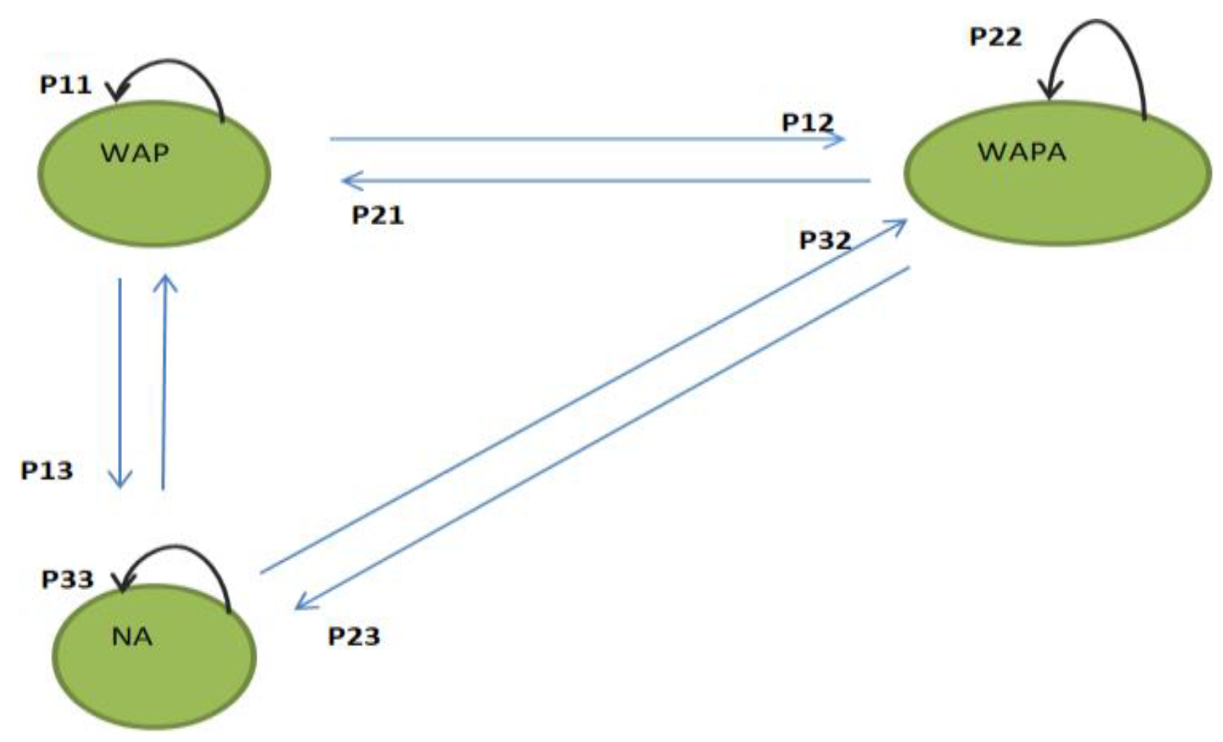
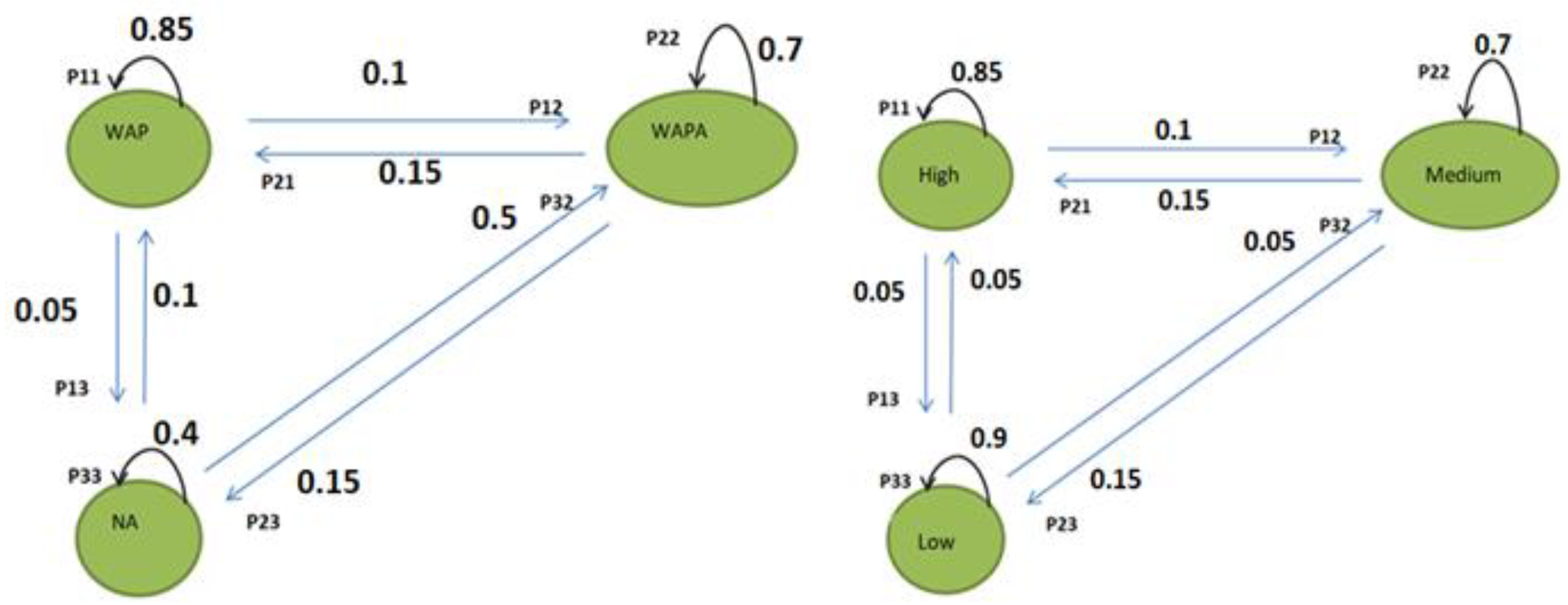
The assumed transition probabilities for WAP, WAPA, and NA from the socio-economic survey as well as between High, Medium, and Low are shown in Figure 14.

The following are the assumed results of the energy survey in the unelectrified village:

(i)

Using the households’ current energy use and their economic state, wellbeing, and future appliance wish list, the households are classified into groups 1, 2, and 3 as in

Table 3. Household distribution in the unelectrified village.

Group	No. of Households
Group 1:	65
Group 2:	25
Group 3:	10

. An average daily load is assigned.

$$\left[\begin{array}{c}Hig{h}_0\\ Mediu{m}_0\\ Lo{w}_0\end{array}\right]=\left[\begin{array}{c}0.1\\ 0.25\\ 0.65\end{array}\right]$$

(21)

$$\left[\begin{array}{c}Hig{h}_n\\ Mediu{m}_n\\ Lo{w}_n\end{array}\right]=\left[\begin{array}{ccc}0.85& 0.15& 0.05\\ 0.1& 0.7& 0.05\\ 0.05& 0.15& 0.9\end{array}\right]\left[\begin{array}{c}Hig{h}_{n-1}\\ Mediu{m}_{n-1}\\ Lo{w}_{n-1}\end{array}\right]$$

(22)

(ii)

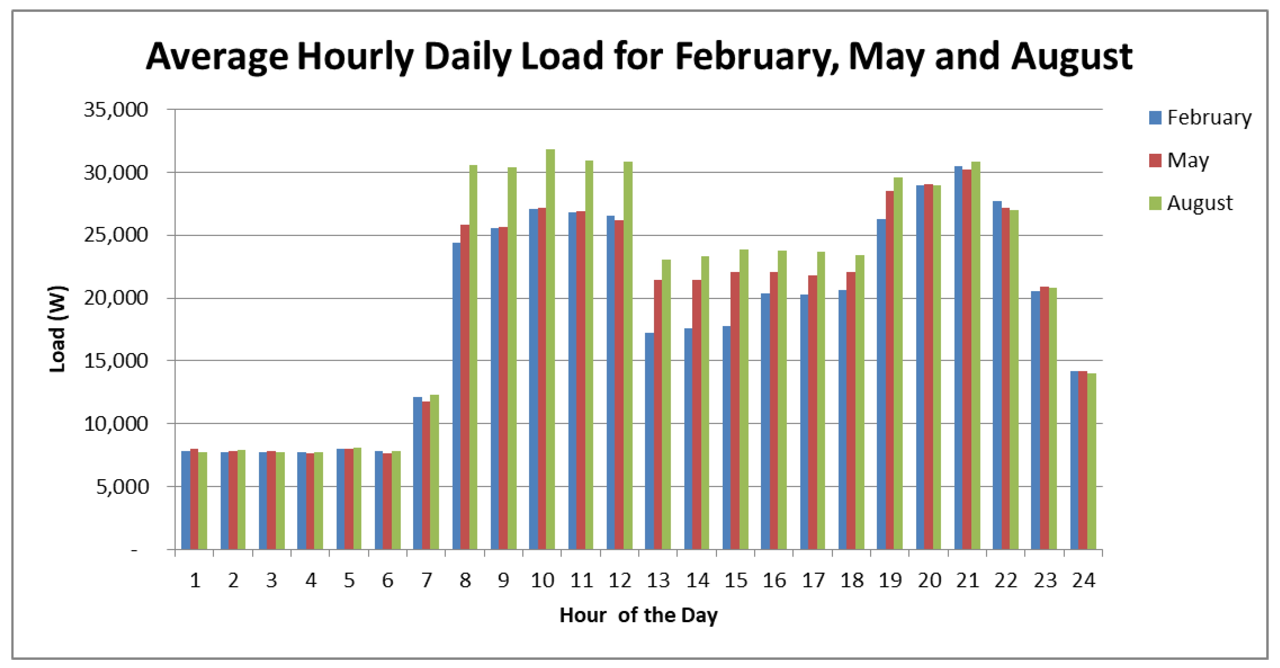
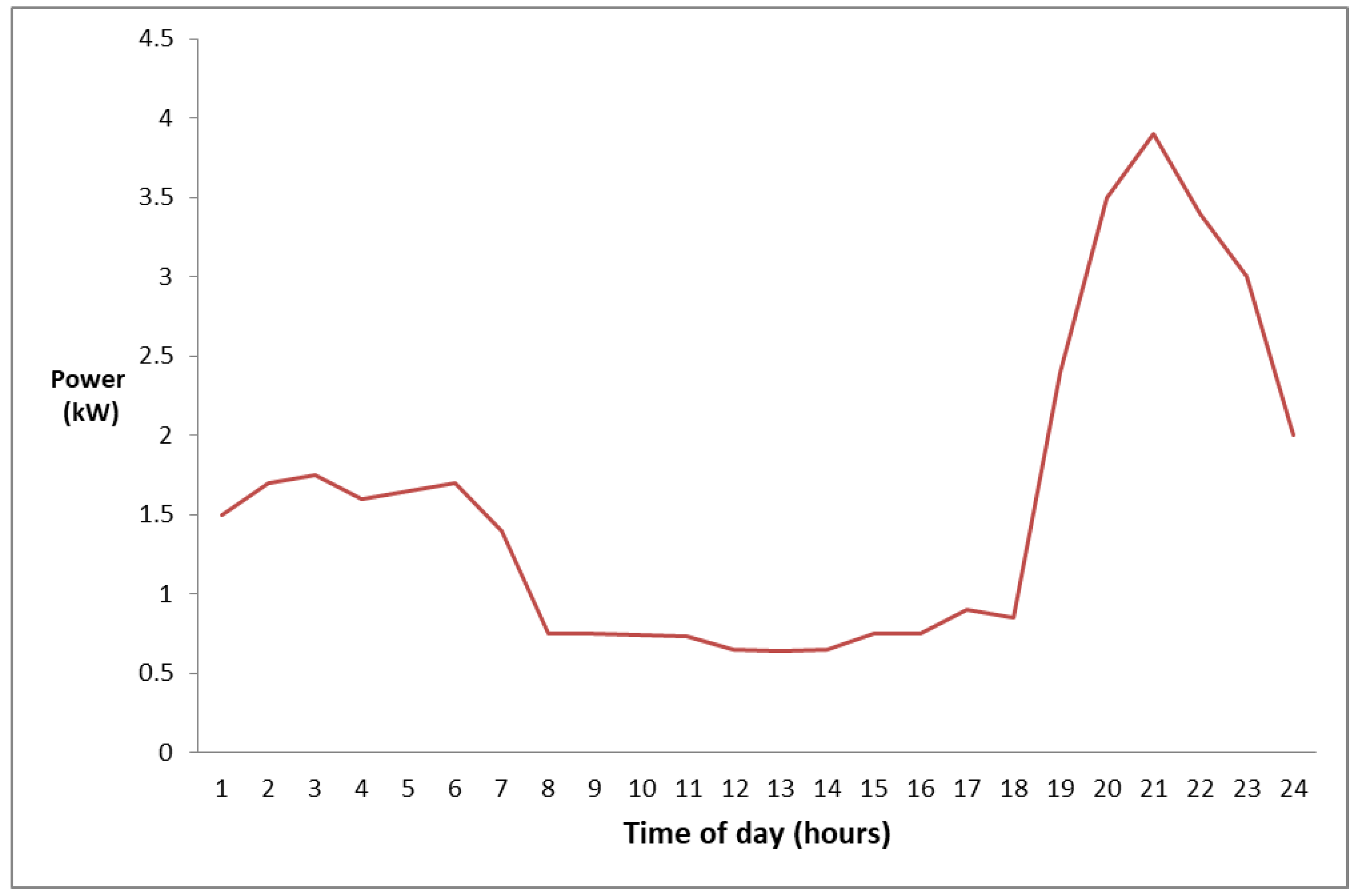
Assuming that all households are to be electrified and the microgrid is designed taking into consideration load growth over a period of 5 years, the load profile will be as shown in Figure 15. The average daily load is 22.1 kWh, and the peak is 5 kWh.

$$\left[\begin{array}{c}Hig{h}_5\\ Mediu{m}_5\\ Lo{w}_5\end{array}\right]=\left[\begin{array}{c}0.27\\ 0.18\\ 0.55\end{array}\right]$$

(23)

(iii)

Assuming that 32% are WAP, 48% are WAPA, and 20% are NA, if the socio-economic characteristics in Village_1 and Village_2 are similar, transition probabilities for Village_1 apply to Village_2.

$$\left[\begin{array}{c}{\mathit{WAP}}_0\\ {\mathit{WAPA}}_0\\ {\mathit{NA}}_0\end{array}\right]=\left[\begin{array}{c}0.32\\ 0.48\\ 0.2\end{array}\right]$$

(24)

$$\left[\begin{array}{c}{\mathit{WAP}}_n\\ {\mathit{WAPA}}_n\\ {\mathit{NA}}_n\end{array}\right]=\left[\begin{array}{ccc}0.85& 0.15& 0.1\\ 0.1& 0.7& 0.5\\ 0.05& 0.15& 0.4\end{array}\right]\left[\begin{array}{c}{\mathit{WAP}}_{n-1}\\ {\mathit{WAPA}}_{n-1}\\ {\mathit{NA}}_{n-1}\end{array}\right]$$

(25)

$$\left[\begin{array}{c}{\mathit{WAP}}_5\\ {\mathit{WAPA}}_5\\ {\mathit{NA}}_5\end{array}\right]=\left[\begin{array}{c}0.45\\ 0.41\\ 0.14\end{array}\right]$$

(26)

The results show that by the 5th year, the percentage of customers with the ability to always pay for electricity will have increased from 32% in year 1 to 45%. The percentage of customers not able to pay will have reduced from 20% in year 1 to 14%. This increase in load may be attributed to the improvement in the socio-economic status of the community, such as an increase in small and medium enterprises and the purchase of more appliances. Moreover, by the 5th year, 41% will irregularly pay. If the microgrid is designed for those who will regularly and irregularly pay, this is 86% of the households. Basing on the transition between High, Medium, and Low, 27% of these connected users will be considered as High users, 18% Medium, and 40% Low. The resultant profile is shown in Figure 15. The average daily load is 21.9 kWh, and the peak is 5.1 kW.

(iv)

Assuming the socio-economic characteristics of Village_1 and Village_2 are different, resulting in different total scores for each village, the ratio of the total score of village 2 to village 1 in this case study is 70%; therefore, the electricity adoption rate for Village_2 is assumed to be 30% slower than that of Village_1. The transition probabilities drivers P21, P31, and P32 are reduced by 30%, and the probabilities P12, P13, and P23 are increased by 30%.

$$\left[\begin{array}{c}{\mathit{WAP}}_n\\ {\mathit{WAPA}}_n\\ {\mathit{NA}}_n\end{array}\right]=\left[\begin{array}{ccc}0.81& 0.1& 0.07\\ 0.13& 0.7& 0.35\\ 0.06& 0.2& 0.58\end{array}\right]\left[\begin{array}{c}{\mathit{WAP}}_{n-1}\\ {\mathit{WAPA}}_{n-1}\\ {\mathit{NA}}_{n-1}\end{array}\right]$$

(27)

$$\left[\begin{array}{c}{\mathit{WAP}}_5\\ {\mathit{WAPA}}_5\\ {\mathit{NA}}_5\end{array}\right]=\left[\begin{array}{c}0.32\\ 0.43\\ 0.25\end{array}\right]$$

(28)

$$\left[\begin{array}{c}{\mathit{High}}_5\\ {\mathit{Medium}}_5\\ {\mathit{Low}}_5\end{array}\right]=\left[\begin{array}{c}0.18\\ 0.16\\ 0.66\end{array}\right]$$

(29)

Designing for those who will regularly and irregularly pay means 75% of the houses will be connected. Of these, 18% are High users, 16% Medium, and 66% Low. The resultant load profile is shown in Figure 15. The average daily load is 19.2 kWh, and the peak load is 4.5 kW.

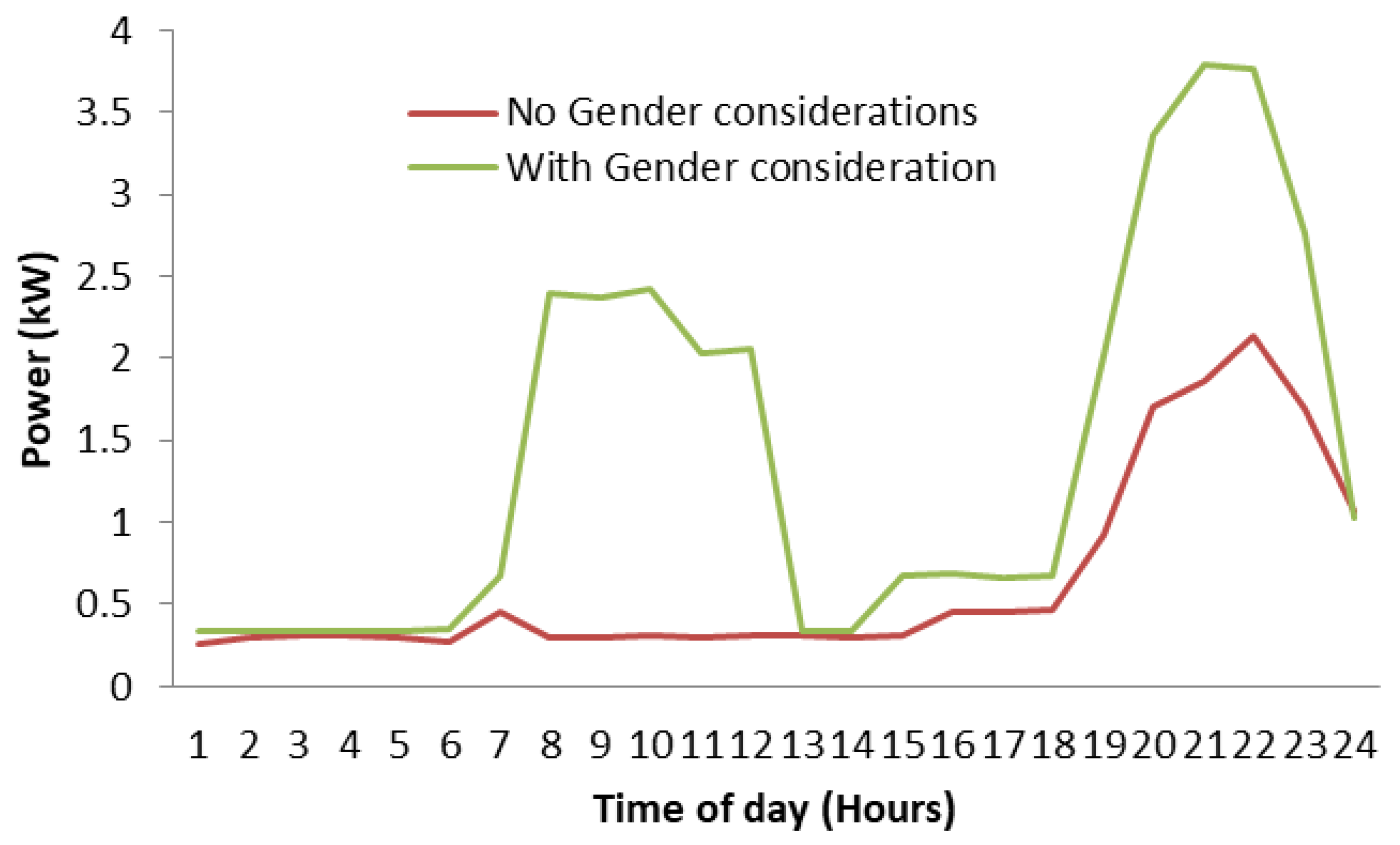
4.3. Effect of Gender on the Resultant Load Profile

Consider a hypothetical village with characteristics as defined in [13,32,33,34]. Assume that the community has 100 houses and a milling machine. Further assume that only men were involved in the energy needs survey, and therefore, women’s interests were not considered during household electrification. In addition, assume that women were not involved in the community income-generating activities as fully discussed in [13]. As presented in [13], the households’ ability to pay is distributed as 32% WAP, 48% WAPA, and 20% NA. The distribution in regards to consumption into High, Medium, and Low categories is 10%, 25%, and 65%, respectively. The average daily consumptions for High, Medium, and Low are assumed to be 350, 200, and 100 Wh, respectively. The transition matrix for customer’s ability to pay and that for their energy consumption transitions as obtained from the survey are assumed to be equal. The probability of a customer staying in the initial state (P11, P22, P33) is high which means that transitioning among other states as indicated by P12, P21, P13, P31, P23, and P32 is low. Equations (30)–(32) represent the transition matrix and the initial state values for WAP, WAPA, NA, High, Medium, and Low.

$$\mathrm{Transition}\mathrm{Matrix}=\left[\begin{array}{ccc}0.8& 0.15& 0.1\\ 0.1& 0.7& 0.2\\ 0.1& 0.15& 0.7\end{array}\right]$$

(30)

$$\left[\begin{array}{c}{\mathit{WAP}}_0\\ {\mathit{WAPA}}_0\\ {\mathit{NA}}_0\end{array}\right]=\left[\begin{array}{c}0.32\\ 0.48\\ 0.2\end{array}\right]$$

(31)

$$\left[\begin{array}{c}{\mathit{High}}_0\\ {\mathit{Medium}}_0\\ {\mathit{Low}}_0\end{array}\right]=\left[\begin{array}{c}0.1\\ 0.25\\ 0.65\end{array}\right]$$

(32)

$$\left[\begin{array}{c}{\mathit{WAP}}_5\\ {\mathit{WAPA}}_5\\ {\mathit{NA}}_5\end{array}\right]=\left[\begin{array}{c}0.38\\ 0.33\\ 0.29\end{array}\right]$$

(33)

$$\left[\begin{array}{c}{\mathit{High}}_5\\ {\mathit{Medium}}_5\\ {\mathit{Low}}_5\end{array}\right]=\left[\begin{array}{c}0.34\\ 0.34\\ 0.32\end{array}\right]$$

(34)

Assuming that the designers of the microgrid decide to consider customers in the categories of WAP and WAPA for load demand of 5 years due to load growth, then the percentage of households that will be electrified will be 71%. The consumption distribution of these electrified households will be 34% High energy consumers, 34% Medium consumers, and 32% will fall into the Low energy consumption category. This is as shown in Equations (33) and (34). Assessing the electrified village against the gender-related indicators gives an overall score of 15 hence representing an average score of 2 per indicator.

Consider another hypothetical village (unelectrified) with the same setup but with a score of 5 for each of the gender-related indicators. The total assessment score for this village against the gender-related indicators would be 35 and the resulting $S_e$calculated using (14) would be 2.33. This implies that the electricity adoption rate for Village_2 is taken to be 2.33 times higher than that of Village_1. The transition probabilities for this unelectrified village are thus determined by increasing the transition probabilities drivers P21, P31, and P32 of the electrified village by the ratio of 233% and reducing the probabilities P12, P13, and P23 by the ratio of 233% which results in the matrix below.

$$\mathrm{Transition}\mathrm{Matrix}=\left[\begin{array}{ccc}1& 0.35& 0.23\\ 0& 0.65& 0.47\\ 0& 0& 0.3\end{array}\right]$$

(35)

$$\left[\begin{array}{c}WA{P}_5\\ WAP{A}_5\\ N{A}_5\end{array}\right]=\left[\begin{array}{c}0.91\\ 0.09\\ 0\end{array}\right]$$

(36)

$$\left[\begin{array}{c}Hig{h}_5\\ Mediu{m}_5\\ Lo{w}_5\end{array}\right]=\left[\begin{array}{c}0.87\\ 0.13\\ 0\end{array}\right]$$

(37)

The microgrid design, in this case, would consider electrification of all the households and the consumption distribution will be 87% High consumption, and 13% Medium consumption. The resultant profiles of the average daily load obtained are shown in Figure 16.

The load profile without gender considerations has a small morning peak and a large evening peak. This could be connected to the men’s availability at home, and hence, the consumption could be due to the men’s use of specific appliances during these time periods. When gender is considered, the resultant load profile has significant morning and evening peaks. This is attributed to the use of appliances during the day such as flat irons, radio, and at times TV. Based on [33,34], it has been assumed that the operations and management of the community maize mill are predominantly carried out by men, and women are not involved. Its performance according to [33,34] is poor and it is not embraced by the women in the community. It has therefore been assumed that for each year, there is a 50% probability that the maize mill will be in WAP state, and the transition from WAP to WAPA or NA is each specified at 0.25. Once the state is WAPA, there is a higher chance that the maize mill will transition to NA than the chance of transitioning to WAP. Once the system is in NA, the probability of transitioning to either WAP or WAPA is very low. These assumptions are represented in (38).

$$\mathrm{Transition}\mathrm{Matrix}=\left[\begin{array}{ccc}0.5& 0.1& 0.1\\ 0.25& 0.65& 0.1\\ 0.25& 0.25& 0.8\end{array}\right]$$

(38)

Assuming an ability to pay initial state of 98% WAP, 2% WAPA and 0% NA in Year 1, the corresponding state at Year 5 is 17% WAP, 30% WAPA and 52% NA. When all gender considerations are met, the Transition matrix is as presented in (39) and will consequently result in 99% WAP in the fifth year. This indicates that the maize mill was maintained in the WAP state for 5 years.

$$\left[\begin{array}{ccc}1& 0.35& 0.23\\ 0& 0.65& 0.47\\ 0& 0& 0.3\end{array}\right]$$

(39)

From this result, it is observed that consideration of gender can lead to a more sustainable system comprising of income-generating activities. When gender aspects are not considered, it may not be possible over time to sustain the rural community’s income-generating activities that were initially installed.

5. Conclusions

In this paper a new approach to electrical load estimation in the design of off-grid rural electrification systems has been has presented. This new approach enhances the existing methods for load estimation. The proposed approach uses stochastic methods to more accurately model uncertainty in the load. Reduction of the estimation error that arises from inaccurate appliance input from energy surveys is achieved by basing the proposed method on known consumption from similar communities. A consideration of socio-economic and gender characteristics of the rural area that is to be electrified is used in the new approach, thus giving a more exact estimation of the load demand. The method has shown that there is a significant impact on the electrical load profiles as a result of gender considerations in the load estimation process. The results have shown a higher consumption when gender is considered. The peak consumption value was about 50% higher when gender was considered than that realised when gender was not considered. While the illustration of the proposed approach in this study was carried out on a sample rural community of 100 homes in Sub-Saharan Africa, with appropriate available data, it can be easily applied to a larger community. However, it is important to point out that the results obtained cannot be generalised as they depend on the social and cultural context of the communities and moreover only one sample community was investigated. The results will vary between communities and between rural and urban areas as well as between regions of the world. The results will also vary when the climate, weather conditions, occurrence, and frequency of disturbances caused by wind, rain, snow, and low temperatures among others are taken into account. Despite limited comparative analyses, the research has shown that the proposed load estimation method addresses the gap that exists between engineering modelling and social science theory. Furthermore, the proposed load estimation approach has provided a way of measuring and estimating load growth or change over time (year-to-year), hence making it easy for the microgrid planners to design systems that are well-targeted to the community to be served. The new approach has shown that the Markov chain process can suitably be used to investigate the effect of changes in customer habits on the estimated load so as to be able to determine year-to-year load profiles.

References

1. Mandelli, S. Strategies for Access to Energy in Developing Countries: Methods and Models for Off-Grid Power Systems Design. Ph.D. Thesis, Politecnico Milano, Milan, Italy, 2015; pp. 1–203. [Google Scholar]
2. Willis, H.L. Characteristics of Distribution Loads. In Electrical Transmission and Distribution Reference Book; Chapter 24; ABB Power T&D Company Inc.: Raleigh, NC, USA; pp. 784–808.
3. Bhattacharyya, S. Review of alternative methodologies for analysing off-grid electricity supply. Renew. Sustain. Energy Rev. 2012, 16, 677–694. [Google Scholar] [CrossRef]
4. Mandelli, S.; Merlo, M.; Colombo, E. Novel procedure to formulate load profiles for off-grid rural areas. Energy Sustain. Dev. 2016, 31, 130–142. [Google Scholar] [CrossRef]
5. Blodgett, C.; Dauenhauer, P.; Louie, H.; Kickham, L. Accuracy of energy-use surveys in predicting rural mini-grid user consumption. Energy Sustain. Dev. 2017, 41, 88–105. [Google Scholar] [CrossRef] [Green Version]
6. Solar Energy International. Photovoltaics Design and Installation Manual; New Society Publishers: Gabriola Island, BC, Canada, 2004. [Google Scholar]
7. Sakiliba, S.K.; Hassan, A.S.; Wu, J.; Saja, E.; Ademi, S. Assessment of Stand-Alone Residential Solar Photovoltaic Application in Sub-Saharan Africa: A Case Study of Gambia. J. Renew. Energy 2015, 2015, 1–10. [Google Scholar] [CrossRef] [Green Version]
8. Ishaq, M.; Ibrahim, U.H. Design of an Off Grid Photovoltaic System: A Case Study of Government Technical College, Wudil, Kano State. Int. J. Sci. Technol. Res. 2013, 2, 12. [Google Scholar]
9. Saleh, U.A.; Haruna, Y.S.; Onuigbo, F.I. Design and Procedure for Stand-Alone Photovoltaic Power System for Ozone Monitor Laboratory at Anyigba, North Central Nigeria. Int. J. Eng. Sci. Innov. Technol. 2015, 4, 41–52. [Google Scholar]
10. Soufi, A.; Chermitti, A.; Triki, N.B. Sizing and Optimization of a Livestock Shelters Solar Stand-Alone Power System. Int. J. Comput. Appl. 2013, 71, 975–8887. [Google Scholar] [CrossRef]
11. Abu-Jasser, A. A stand-alone photovoltaic system, case study: A residence in Gaza. J. Appl. Sci. Environ. Sanit. 2010, 5, 81–91. [Google Scholar]
12. Oko, C.; Diemuodeke, E.; Omunakwe, E.; Nnamdi, E. Design and Economic Analysis of a Photovoltaic System: A Case Study. Int. J. Renew. Energy Dev. 2012, 1, 65–73. [Google Scholar] [CrossRef]
13. Namaganda-Kiyimba, J.; Mutale, J. Gender Considerations in Load Estimation for Rural Electrification. In Proceedings of the 2020 IEEE Conference on Technologies for Sustainability (SusTech), Santa Ana, CA, USA, 24–25 April 2020; pp. 263–270. [Google Scholar]
14. Rojas-Zerpa, J.C.; Yusta, J.M. Methodologies, technologies and applications for electric supply planning in rural remote areas. Energy Sustain. Dev. 2014, 20, 66–76. [Google Scholar] [CrossRef]
15. Grandjean, A.; Adnot, J.; Binet, G. A review and an analysis of the residential electric load curve models. Renew. Sustain. Energy Rev. 2012, 16, 6539–6565. [Google Scholar] [CrossRef]
16. Nandi, S.K.; Ghosh, H.R. Prospect of wind–PV-battery hybrid power system as an alternative to grid extension in Bangladesh. Energy 2010, 35, 3040–3047. [Google Scholar] [CrossRef]
17. Celik, A. Effect of different load profiles on the loss-of-load probability of stand-alone photovoltaic systems. Renew. Energy 2007, 32, 2096–2115. [Google Scholar] [CrossRef]
18. Boait, P.; Advani, V.; Gammon, R. Estimation of demand diversity and daily demand profile for off-grid electrification in developing countries. Energy Sustain. Dev. 2015, 29, 135–141. [Google Scholar] [CrossRef] [Green Version]
19. Riva, F.; Ahlborg, H.; Hartvigsson, E.; Pachauri, S.; Colombo, E. Electricity access and rural development: Review of complex socio-economic dynamics and causal diagrams for more appropriate energy modelling. Energy Sustain. Dev. 2018, 43, 203–223. [Google Scholar] [CrossRef]
20. Hartvigsson, E.; Ahlgren, E.O. Comparison of load profiles in a mini-grid: Assessment of performance metrics using measured and interview-based data. Energy Sustain. Dev. 2018, 43, 186–195. [Google Scholar] [CrossRef]
21. Narayan, N.; Qin, Z.; Popovic-Gerber, J.; Diehl, J.C.; Bauer, P.; Zeman, M. Stochastic load profile construction for the multi-tier framework for household electricity access using off-grid DC appliances. Energy Effic. 2018, 13, 197–215. [Google Scholar] [CrossRef] [Green Version]
22. Williams, N.J.; Jaramillo, P. Electricity consumption and load profile segmentation analysis for rural microgrid customers in Tanzania. In Proceedings of the 2018 IEEE PES/IAS PowerAfrica Conference, Cape Town, South Africa, 28–29 June 2018; pp. 360–365. [Google Scholar]
23. Andersson, M.; Andersson, C. A Simple Load Estimation Model for Rural Electrification in Tanzania. Master’s Thesis, Lund University, Lund, Sweden.
24. Uganda Bureau of Statistics. Uganda National Household Survey 2016/2017 Report; Uganda Bureau of Statistics: Kampala, Uganda, 2017; p. 300.
25. Sprei, F. Characterization of Power System Loads in Rural Uganda. Master’s Thesis, Lund University, Lund, Sweden, 2002; pp. 1–74. [Google Scholar]
26. Blennow, H.; Bergman, S. Method for Rural Load Estimations—A Case Study in Tanzania. Master’s Thesis, Lund Institute of Technology, Lund, Sweden, 2004; pp. 1–5. [Google Scholar]
27. Piper, S.; Martin, W. Assessing the financial and economic feasibility of rural water system improvements. Impact Assess. Proj. Apprais. 1999, 17, 171–182. [Google Scholar] [CrossRef] [Green Version]
28. Pfeifer, P.E.; Carraway, R.L. Modeling customer relationships as Markov chains. J. Interact. Mark. 2000, 14, 43–55. [Google Scholar] [CrossRef]
29. Katre, A.; Tozzi, A.; Bhattacharyya, S. Sustainability of community-owned mini-grids: Evidence from India. Energy Sustain. Soc. 2019, 9, 1. [Google Scholar] [CrossRef] [Green Version]
30. Katre, A.; Tozzi, A. Assessing the Sustainability of Decentralized Renewable Energy Systems: A Comprehensive Framework with Analytical Methods. Sustainability 2018, 10, 1058. [Google Scholar] [CrossRef] [Green Version]
31. Ministry of Energy and Mineral Development and Uganda Bureau of Statistics. Uganda Rural-Urban Electrification Survey, 2012; Ministry of Energy and Mineral Development and Uganda Bureau of Statistics: Kampala, Uganda, 2014; p. 163.
32. Winther, T.; Ulsrud, K.; Saini, A. Solar powered electricity access: Implications for women’s empowerment in rural Kenya. Energy Res. Soc. Sci. 2018, 44, 61–74. [Google Scholar] [CrossRef]
33. García, V.G.; Bartolomé, M.M. Rural electrification systems based on renewable energy: The social dimensions of an innovative technology. Technol. Soc. 2010, 32, 303–311. [Google Scholar] [CrossRef]
34. The Value of Women’s Time in Ethiopia’s Forests. Available online: https://www.technoserve.org/blog/the-value-of-womens-time-in-ethiopias-forests (accessed on 30 April 2019).
Figure 1. Improved load modelling approach framework.
Energies 14 05505 g001
Figure 2. Flow chart for calculation of hourly percentage of daily load.
Energies 14 05505 g002
Figure 3. Ability to pay factors for WAP, WAPA, and NA.
Energies 14 05505 g003
Figure 4. Possible transitions between WAP, WAPA, NA states for customers.
Energies 14 05505 g004
Figure 5. Possible transitions between High, Medium, and Low consumption.
Energies 14 05505 g005
Figure 6. Flow chart for calculation of energy consumption at each hour.
Energies 14 05505 g006
Figure 7. Average hourly daily load variation for February, May, and August.
Energies 14 05505 g007
Figure 8. Load profile for household category.
Energies 14 05505 g008
Figure 9. Load profile for the maize mill in August, May, and February.
Energies 14 05505 g009
Figure 10. Load profiles for the barbershop (a), school (b), and health centre (c).
Energies 14 05505 g010
Figure 11. Measured load profile from [25].
Energies 14 05505 g011
Figure 12. Estimated load profile for new village to be electrified.
Energies 14 05505 g012
Figure 13. Household load profiles.
Energies 14 05505 g013
Figure 14. Transition for WAP, WAPA, and NA and High, Medium, and Low.
Energies 14 05505 g014
Figure 15. Load profiles for different socio-economic characteristics.
Energies 14 05505 g015
Figure 16. Resulting load profiles with and without gender considerations.
Energies 14 05505 g016