Article

Influence of Swirl Clocking on the Performance of Turbine Stage with Three-Dimensional Nozzle Guide Vane

1
School of Mechanical Engineering, Pusan National University, Pusan 46241, Korea
2
Department of Mechanical Engineering, Virginia Polytechnic Institute and State University, Blacksburg, VA 24061, USA
3
Gas Turbine Center, Doosan Heavy Industries & Construction, Changwon 51711, Korea
*
Author to whom correspondence should be addressed.
Energies 2021, 14(17), 5503; https://doi.org/10.3390/en14175503
Submission received: 11 August 2021 / Revised: 28 August 2021 / Accepted: 31 August 2021 / Published: 3 September 2021

Abstract

:
The effect of the swirl clocking on three-dimensional nozzle guide vane (NGV) is investigated using computational fluid dynamics. The research reports the loss characteristics of leaned and swept NGVs and the influence of swirl clocking. The three-dimensional NGVs are built by stacking the same 2D profile along different linear axes, characterized by different angles with respect to the normal or radial direction: ε = −12° ~ +12° for the leaned and γ = −5° ~ +10° for the swept airfoils. A total of 40 models are analyzed to study the effects of lean and sweep on aerodynamic performance. To investigate the influence of swirl clocking, the analysis cases include the center of the swirl that was positioned at the leading edge as well as the middle of the passage. The prediction results show that the relationship of the changes in mass flow rate and throat area are not monotonic. Further observation confirms the redistribution of loading and flow angle under different lean and sweep angles; thus, three-dimensional design is a key influencing factor on aerodynamic performance. In the presence of swirl clocking, NGV performance is changed significantly and the findings offer new insight and opportunities to improve three-dimensional NGV airfoil design.

1. Introduction

The Nozzle Guide Vane (NGV) of a turbine experiences a highly turbulent combustion flow with a complicated swirl structure [1,2]. The role of NGV is to turn the flow to the right angle for downstream rotor and stages while controlling the flow rate through its throat area. In addition, further cooling and structural requirements should be considered to withstand high pressure and temperature operating conditions. Therefore, this motivates researchers to develop robust approaches for improving overall efficiency by controlling flow through NGV. One of which is to implement lean and sweep angles to the NGV. Lean is a stacking-line modification in which NGV sections are moved relative to each other in the circumferential direction. For sweep, the modification applies to the axial direction. Therefore, the influence of lean, sweep and swirl on the three-dimensional aerodynamics of turbine passage is of great interest to researchers. The very early concept of radial airfoil stacking was introduced about sixty years ago. Straight lean and compound lean have been recognized as an effective way to control the reaction, loading and secondary flows [3,4,5,6,7,8,9,10,11]. It has been reported that the straight lean and compound lean can reorganize the vortices and reduce the secondary flow loss. As a result, the secondary flow loss decreased remarkably by using appropriate leaned blades [12,13,14,15,16]. The sweep commonly occurred because the meridional passage of the main annulus is not typically at a constant radius, whereas the NGV is stacked on a near radial line in the meridional views. The secondary flow structure and the pressure distribution of the NGV passage are closely linked so that the sweep angle affects the secondary loss mechanism [17,18]. However, the sweep angle may simply shift the loss from the endwall region to mid-span [19,20]. The potential impact and limitation of the understanding were reviewed as the technology developed [21,22]. It has been almost twenty years since the advanced computational fluid dynamics (CFD) and experimental approach have been brought into turbomachinery research. Comprehensive results from experiments and CFD are reported to enhance the understanding of the root cause [3,4,5,6,7,9,10,11,12,13,14,15,17,18,19,20,21,22,23,24,25,26,27,28,29]. Furthermore, the design optimization approach is being applied to offer more complicated control of design parameters [8,16,30].
While the previous research on lean and sweep reported its influence on three-dimensional aerodynamics of airfoil passage, there is rarely any report in conjunction with swirl clocking. Similarly, the research on the swirl effect on NGV aerodynamic performance [21,23,24,25,26] did not consider the lean and sweep. The present study aims to investigate the influence of the three-dimensionality of NGV on the turbine stage considering more realistic operation conditions. Therefore, a 1.5 stage turbine with three-dimensional NGV airfoil is modeled for simulating the swirl clocking. A series of CFD is conducted to (1) confirm the findings from early research and (2) reveal the further understanding of the impact of swirl clocking on the stage performance. A parametric geometry is created for the present study. The parameters to vary the NGV geometry are the angles of lean (+12 ~ −12, Δ = 6°), compound lean (+12 ~ −12, Δ = 6°), and sweep (+10 ~ −5, Δ = 5°). In addition, the study extended to include the swirl clocking by positioning the swirl core at the leading edge and passage center of NGV. For the analysis, the variation of the shape of NGV is achieved by using in-house tools. Then, the produced airfoil geometries are transferred to TurboGrid (Version 19.2 R2, ANSYS Inc., Canonsburg, PA, USA) to generate computational grids. In CFX (Version 19.2 R2, ANSYS Inc., Canonsburg, PA, USA), the properties of combustion gas and total to static pressure ratio are applied for the calculation. Uniform inlet total temperature and adiabatic walls are assumed. To model turbulence, SST (Shear Stress Transport) is selected with an inlet freestream turbulence intensity of 5%. In total, 108 cases are analyzed for the present investigation.

2. Computational Model and Approach

A nozzle guide vane of the first stage turbine of an industrial gas turbine is used as a baseline configuration for CFD validation. The airfoil at 50% span height is shown in Figure 1. The NGV has an axial chord of 123.6 mm at 50% span height and a total of 48 airfoils around the annulus. The height of the airfoil is 157.20 mm at the leading edge (LE) and the NGV exit angle is 71.2° at 50% span height. The total to total pressure ratio is 1.86 and the stage efficiency is 91.8%. The inlet Reynolds number is 1.32 × 10⁶ and the exit Mach number at design condition is 0.77 at mid-span height.
The computational domain is shown in Figure 2, which starts from 0.6 Cax upstream of the leading edge (LE) and ends at 0.1 Cax downstream of the trailing edge. The principal geometric parameters of the NGV and boundary conditions utilized in this research are shown in Table 1.
The definition of total to total isentropic efficiency in this paper is
η t = h 02 h 01 h 02 h 01
where η t is total to total isentropic efficiency, h is static enthalpy, respectively.
C p = p 01 ¯ p 02 0.5 ρ 2 u 2 2
where Cp is total pressure loss coefficient, p0 is total pressure, ρ is density and u is velocity.
Q = C Q Ω 2 S 2
where CQ = 0.25, S is the absolute value of the strain rate (s−1) and is the absolute value of vorticity (s−1).
For this systematic parametric study, a total of 40 NGV configurations applying straight lean, compound lean and sweep angles are constructed. The baseline model has straight lean = 0°, and sweep = 0°. The parametric geometry is based on the baseline NGV configuration. The geometrical representation of NGV consists of a total of 11 sections including hub, mean and tip. Each cross section of the airfoil represented by the pressure side (PS) and suction side (SS) is designed using the Pritchard 11-parameter method [31]. The baseline NGV geometry uses a simple radial stack around the NGV trailing edge with no lean and sweep. By changing the shape of stacking line, a new NGV model is obtained.
The other 39 NGVs are constructed by applying different straight lean, compound lean and sweep. In the case of straight lean models, the stacking lines are leaned in the circumferential direction (Figure 3a). The compound lean has an elliptical tangential stacking profile within the angle inclination at both end-walls (Figure 3a). Positive and negative straight lean angles are applied to study its influence and the same approach is applied to the airfoils with compound lean angles. The sweep is defined as the deviation of the stacking axis of the airfoil from a line perpendicular to the axisymmetric stream surface in the meridional view (Figure 3b). As summarized in Table 2, the sweep angle chosen for the present investigation is in the range of −5° ~ +10°. For lean angle, a slightly wider range angle of −12° ~ +12° is selected. These lean angles provide sufficient geometry variation to drives the changes in aerodynamic characteristics including loading, secondary flow and mass-flow distribution. Figure 4 shows the overlapped cross-sectional geometries of four selected three-dimensional NGV airfoils.
The computational domain and mesh (5 × 10⁶ nodes) and the station number of the turbine stage are shown in Figure 2 and Figure 5, respectively. The steady-state calculations were conducted using the commercial CFD package, CFX, which solves the Reynolds-averaged Navier–Stokes equations using a finite-volume, node-centered approach with high-resolution schemes for convective fluxes and implicit time integration. The k-ω SST turbulent is used and under the no-slip wall conditions. A periodic boundary condition is applied in the circumferential interface. The mixing plane approach is adopted to the interfaces between stator and rotor as shown in Figure 5. The boundary layer is resolved by achieving the y+ of approximately 1 throughout the domain as required to resolve the near-wall region and to avoid the use of wall functions. The difference in NGV efficiency predictions due to mesh density is in the order of 10−4. Figure 6 compares numerical and experimental results in terms of the surface pressure distribution and total pressure loss at vane exit (z/Cax = 1.1). Figure 6 shows good agreement between predicted and measured data.
To study swirl clocking, the swirl intensity which is characterized by swirl number, SN (the ratio of the axial momentum flux and a characteristic radius [32]) is implemented for the present study. The applied inlet swirl profile and clocking positions (Figure 7) are representing a swirl number of approximately 0.5. The overall analysis matrix is shown in Table 3.
S N = u ¯ w ¯ r 2 d r R u ¯ 2 r d r

3. Results

3.1. Stage Performance with and without Swirl Clocking

Figure 8 compares the stage efficiencies of a total of 108 cases analyzed for the present study. For comparison, the results of straight lean with sweep are collected in Figure 8a, and compound lean with sweep are shown in Figure 8b, respectively. The baseline airfoil geometry (lean angle = sweep angle = 0°) of NGV is highlighted using a solid green-colored triangle. The variation in lean angle (±12°) is noted in the figure. The changes in sweep angle (−5° ~ +10°) is distinguished by different colors. Finally, the case of swirl center aligned at the leading edge of NGV is expressed using a dotted line. The dash-dotted line is used to represent the alignment of the swirl center in the middle of passage (between leading edges). In Figure 8a, the group of the triangle symbols in solid line shows the highest efficiency. These are the cases without swirl (No swirl) but showing the influence of lean and sweep angles to stage efficiency. Both positive lean and sweep angles improve stage efficiency but negative angles reduce the efficiency. The improvement due to the positive sweep angle (+10°) is the highest (0.127%p) when there is no lean angle applied to the airfoil. A similar observation can be made for the influence of lean angle as the improvement due to positive lean angle (+12°) is the highest (0.174%p) without sweep angle. However, the influence of lean angle is less sensitive to compound lean cases shown in Figure 8b. This characteristic makes compound lean more robust design choice as known. An increase in sweep angle still improves the stage efficiency.
By introducing the swirl clocking, the trend of stage efficiency is changed dramatically (Figure 8). The two swirl clocking positions representing the core of the combustor exit swirl are aligned at (1) the leading edge of NGV and (2) the center of the passage. First of all, the stage efficiency is reduced significantly in general. The maximum reduction is about 1.362%p for the model of SL12 SP10 compared to the no-swirl case. For straight lean cases, in Figure 8a, the stage efficiency curves with a swirl at passage center are simply shifted down. However, the trend with a swirl at leading edge is reversed. The detailed three-dimensional flow field will be followed to explain the difference in loss mechanism.
The models with compound lean angles shown in Figure 8b are less sensitive to the lean angle in the presence of swirl clocking compared to straight lean. However, the influence of the lean angle is recognizable when the swirl center is positioned at the leading edge. The variation in sweep angle influences the stage efficiency in a similar way to the straight lean.
It will also be important to monitor the change in the throat area due to lean and sweep, as it will influence mass flow rate. Figure 9 shows the comparison between the throat area and mass flow rate of all cases. It is interesting to observe that the increase in throat area is not always the cause of the increase in mass flow rate. The slopes of normalized mass flow rate and throat area are different in many cases, except Figure 9d of the straight lean with sweep angle. Nevertheless, the mass flow rate increases as lean and sweep angles increase. Therefore, the increase in stage efficiency of straight lean airfoils is influenced by lean and sweep angles. With compound lean (Figure 9c,d), the variations in throat area and mass flow rate are much smaller than that of the straight lean. This will be one of the reasons for less variation in the stage efficiency due to the lean and sweep.

3.2. Effect of Straight Lean, Compound Lean and Sweep

There are early studies to investigate the influence of lean and sweep angles on turbine aerodynamics [21,22]. Prior to discuss about its combined effect and also swirl clocking, it will be worthwhile to observe the influence of straight lean, compound lean and sweep on the flow field of turbine passage. Figure 10 shows the distribution of total pressure loss coefficient varying those angles. The straight lean of +12° model shows reduction in loss at lower endwall region while the loss is increase near the upper endwall compares to the baseline model. The compound lean model with the same +12° minimizes the loss at the upper endwall region. By applying the sweep angle (10°), the level of loss near the upper endwall region is reduced but the wake is widely spread than the baseline model. The same trend is also observed for the swept airfoils with straight and compound lean angles.
In Figure 11, the circumferentially averaged parameters of flow rate, exit flow angle and total pressure loss coefficient are compared at the exit plane of NGV. The comparison is intended to confirm the findings from the previous researches [5,19,20,23]. Straight lean angle is varied from +12° to −12° with the interval of 6°. Figure 11a–c shows the influence of straight lean angle of +12°, 0° (baseline model) and −12°. The positive lean of 12° (red-colored line) makes more mass flow rate passes through the lower half of the span height so that it leads to under turning of the exit flow. Considering the exit metal angle near the trailing edge in the region of span height of 15% is 70°, it concludes less total pressure loss as shown in Figure 11c. However, the trend is reversed in the upper half of the span height. The observation is changed when the negative lean of 12° (blue-colored line) is applied. For the compound lean, Figure 11d–f, the benefit of the lean angle applies to the lower and upper regions of the span height and keep the flow field of the mid-span region similar to the baseline airfoil. In comparison of positive and negative compound lean models, the positive 12° leaned model (red-colored line) showed reduced loss at the lower and upper regions of the span height. As the results show, the compound leaned airfoil is expected to be more robust design to de-sensitize the overall loss mechanism in turbine passage. For the cases only with sweep angle, Figure 11g–i show the characteristics of the NGV passage flow. The positive sweep angle of 10° increases mass flow rate through the lower 30% of span height and it produces a similar effect as it was observed from the positive straight lean angle of 12°. However, there are two main differences as (1) the location of the highest total pressure loss coefficient is moved upward slightly from lower endwall region and (2) the loss is not high as it was for the positive straight lean angle of 12° in the upper endwall region.
These changes in the flow field are also associated with the changes in the airfoil loading. Figure 12 shows the radial variations of the static pressure distributions of the baseline NGV and blade at 10%, 50% and 90% span heights. It will be regarded as a reference in comparison with other models. The loading distributions of negative and positive 12° of straight lean models are compared in Figure 13. The negative lean angle contributes to make bigger radial changes in the loading distribution while the positive lean angle moves the loading toward the front of the axial chord of the airfoil. The compound leaned NGV shows different characteristics in loading distribution as shown in Figure 14. The positive compound leaned model put more loading in the mid-span region but the negative angle allocated a higher loading towards the upper and lower endwalls. Interestingly, the positive sweep redistributes the loading more toward the front of the airfoil while the negative sweep keeps the loading similar to the baseline but shows slightly higher gradient along the radial direction as compared in Figure 15. Finally, the loading distributions of the two models with maximum and minimum efficiencies are compared in Figure 16.

3.3. Combined Effect of Lean with Sweep

The influence of the combined angles of lean and sweep on aerodynamic characteristics is compared in this section. The comparison is made for the combination of maximum positive (+12°) and negative (−12°) lean angles with sweep angles of 0° and +10°. Figure 17 shows the comparison of circumferentially averaged mass flow rate, exit flow angle, and total pressure loss coefficient due to the combined effect of the straight lean with sweep. It is interesting to observe that the radial variations of the presented parameters are similar to the trend of the individual influence of lean and sweep angles. The superposition of the two effects is what can be seen in the comparison. This trend and comparison are seen also in Figure 18 where the combined effects of compound lean and sweep are compared for the selected angles. Figure 19 shows the static pressure distributions at 10%, 50% and 90% span heights. Comparing Figure 13b and Figure 14b shows the loading distribution by adding the sweep angle of +10°. As observed already, the positive sweep tends to increase the loading at the lower endwall. This influence is added to the combined models as expected. The loading is slightly increased at 10% span height by adding the sweep angle of +10°.
The present data observation provides useful insights on how each of the combined angles of straight and compound lean and sweep influence the aerodynamics characteristics.

3.4. Effect of Swirl Clocking

As observed in Figure 8, the application of the swirl clocking to 3D NGV changed the stage performance characteristics quite dramatically. The two swirl clocking positions are introduced, one at the center of the leading edge and another shifted half of the pitch in the clockwise direction (front view); hence, at the center of passage 1. Figure 20 visualizes the development of vorticity and interaction with passage flow due to the swirl clocking. When the swirl core is aligned to the leading edge of NGV, Figure 20b,e, the vortex (red-coloured) stays on the suction side of NGV and then it is pushed towards the upper endwall (this can be observed from the rear view) as it flows downstream. The development of the counter vortex (blue-colored) is also observed near the upper endwall. From the surface oil flow trajectory, the stagnation lines at the leading edge of both NGVs are strongly deflected toward the pressure side. Figure 20c,f show the vortex structure when the swirl core is aligned at the center of passage 1. The combustor exit swirl remains strong through the center of the passage. The counter vortex is also stronger than the swirl center at the leading edge. The stagnation lines of the leading edge of both NGVs are deflected toward the pressure side. Stronger downwash flow is observed on the pressure surface from the oil flow trajectory. As shown in the results, a stronger vortex on the suction surface of NGV1 is also observed in Figure 20f. These will contribute to increasing secondary flow loss of the cases with the swirl clocking at the passage center.
Another interesting observation from Figure 8 is that the characteristics of the stage performance are reversed when the swirl clocking is positioned at the center of the leading edge. Particularly for the straight lean of −12°, it shows higher stage performance with the swirl cockling at the leading edge than at the passage center. To understand the mechanism, Figure 21 is presented by comparing the influence of the positive and negative lean angles to the swirl clocking. It is clearly seen that the straight lean of −12° splits the combustor swirl from the leading edge so that weaker vortices are passing through the pressure and suction side of the NGV1. With maximum lean and sweep angles, the SL12 SP10 model shows minimum sensitivity to the swirl clocking (see Figure 8). Figure 22 shows the development of the vorticity depends on the swirl clocking positions. It only provides qualitative comparison but shows the strength of vortices of the two swirl clocking cases.
These findings contribute to improving the flow field characterization in the presence of a combustor swirl. Therefore, the traditional understanding and 3D design approach should be reconsidered if swirl clocking is introduced as it dominates the loss mechanism in the turbine passage.

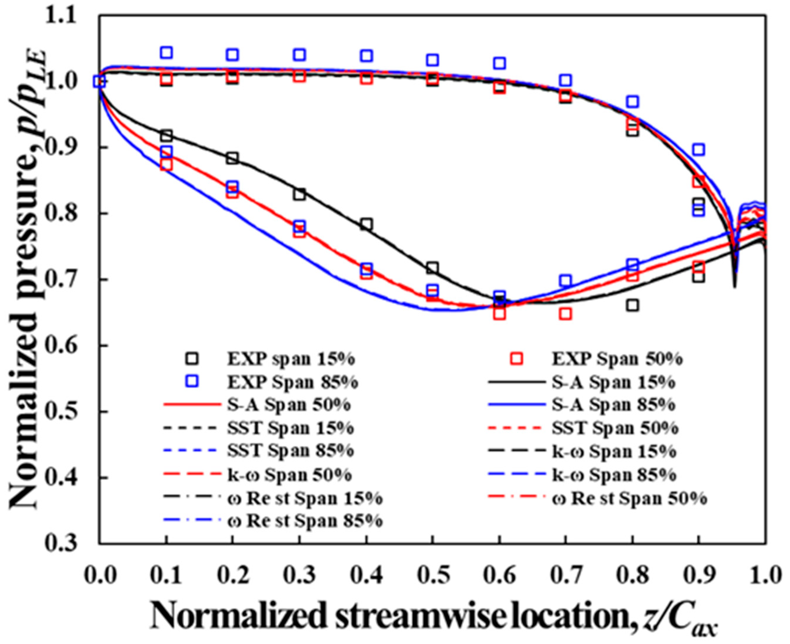
3.5. Downstream of NGV Passages and Mixing Plane

It should be noted that the flows through passage 1 and 2 experience different inlet swirl due to the clocking positions as shown in Figure 23. This shows the combined effect of 3D NGV and swirl clocking on the total pressure loss coefficient at the exit plane of NGV. Comparison with Figure 10 provides clear observation on the influence of the swirl clocking. Although it looks complicated, the previous understanding from Figure 20 supports the analysis of the swirl interaction with 3D NGV models. A similar interaction mechanism drives the flow through the passage so that the loss is more concentrated at the upper endwall and at the center of the passage depends on swirl clocking position.
Figure 24 shows the comparison of circumferentially averaged total pressure loss coefficients for passage 1 (blue-colored line) and 2 (red-colored line). The results show different loss distributions downstream of the two passages as expected from the previous observation. For reference purposes, the loss distribution averaged over the two passages is also presented in a dotted black line. It proves that such an average approach is not appropriate for distinguishing the influence of the inlet swirl on each passage. The solid black line represents the loss distribution of the baseline model without inlet swirl.
The present study also aims to understand the influence of 3D NGV and swirl clocking on stage performance. Hence, the computational domain includes 1.5 stages of the turbine. Ideally, unsteady CFD applying a sliding mesh interface will be more physically representative. However, evaluating the average performance is still meaningful to support the present research interest and saves computational time to complete a large number of calculations. For these reasons, steady CFD with mixing plane interface is applied for the series of calculations. Figure 25 shows the distributions of total pressure loss coefficient at the mixing plane depends on swirl clocking positions. It still captures the key flow characteristics of NGV downstream and passes the effect of wake flow to the computational domain of the blade. As seen in the results, the loss distributions at the exit of the blade are influenced by the swirl clocking. This observation supports the value of the present study applying steady CFD with a mixing plane interface.

3.6. Stage Performance with Swirl Clocking

From Figure 8, it is interesting to observe that the stage performance is strongly influenced by the proposed swirl clocking. Detailed analysis is made for the models showing the highest stage performance at the proposed swirl clocking positions as shown in Table 4. The models performing better than others are with the largest lean (+12°) and sweep (+10°) angles, and also the one with a negative lean angle of −12°. The SP-12 SP10 model shows the highest stage performance when the swirl core is aligned at the leading edge of NGV. In Figure 21, the swirl interaction with 3D NGV was shown to explain the loss mechanism. In this section, the detailed characteristics of the key parameters are presented to confirm the findings from the previous observation.
Figure 26 shows the influence of swirl clocking on the distribution of the total pressure loss coefficient at the exits of NGV. Compared to the distributions shown in Figure 23, the loss is more widely spread as the models have a combined effect of lean and sweep. As observed in Figure 17 and Figure 18, the combined effects can be seen as the superposition of the effect of individual angles. The distorted NGV exit flow continues to influence the blade aerodynamics as shown in Figure 27 and Figure 28.

3.7. Straight Lean (SL+12 SP0, SL-12 SP0 and SL-12 SP10) with Swirl Clocking

To analyze the influence of swirl clocking to 3D NGV, the aerodynamic characteristics of the three models with positive (+12°) and negative (−12°) straight lean angles with and without sweep (+10°) are compared in detail. These are the models with green and black-colored symbols as shown in Figure 8. The stage performances of these three models are changed by the swirl clocking, especially for the model with a negative (−12°) straight lean angle. As shown in Figure 29, the circumferentially averaged total pressure loss coefficients are compared at the exits of NGV and blade. The comparison confirms the influence of negative lean angle (−12°) explored in Figure 21.

3.8. Compound Lean with Swirl Clocking

The SL12 SP10 model showed the highest stage efficiency with no swirl and its performance is less sensitive to the swirl clocking (see Figure 8). Therefore, it is an interesting model to investigate further. For this purpose, the comparison of circumferentially averaged mass flow rate, exit flow angle, and total pressure loss coefficient with swirl clocking is shown in Figure 30. It reflects the vortex formation through the passage shown in Figure 22. With swirl clocking at the leading edge (red-colored lines), spanwise variations of the parameters are more uniform than the results with swirl at passage center and also without swirl. However, the averaged performance is very much the same as shown in Figure 8.
By extending the observation to the compound lean models, it provides better insight into the differences in stage performance. The CL12 SP10 model shows the highest stage efficiency with the proposed swirl clocking (see Figure 8). There is no dramatic change in the stage efficiency as is observed with straight lean models. Furthermore, the lean angle is not sensitive to the stage efficiency except in the cases with swirl clocking at the leading edge. However, the sweep angle is sensitive to the stage efficiency. The mass flow rate and exit flow angle are more uniform and consistent with the two swirl clocking positions as shown in Figure 31. The trends can also be compared with the SL12 SP10 model (see Figure 30). Overall, it can be stated that the compound lean is more robust than the other models, meaning it is less sensitive to the operating conditions.

4. Conclusions

The present study aims to investigate the influence of swirl clocking on turbine stage performance. A total of 108 CFD cases are analyzed to investigate the independent and combined effects of lean, and sweep angles on turbine aerodynamics. Furthermore, the study is extended to consider the influence of swirl clocking. The key findings are summarized as follows.
  • The influence of combined angles of lean and sweep inherits their individual effects.
  • Positive lean and sweep (SL12 SP10 model) shows improved stage performance of +0.208%p with no swirl and +0.101%p with swirl clocking positioned at passage center against the baseline configurations.
  • Negative lean with sweep (SL-12 SP10 model) shows the enhanced stage efficiency of +0.277%p with swirl clocking positioned at the leading edge compared to the baseline model.
  • Compound lean is less sensitive to the swirl clocking while straight lean is strongly influenced.
The present study reveals that there is a strong influence of swirl clocking on the turbine stage performance with 3D NGV. Therefore, designers are asked to consider realistic operating conditions and reflect the findings from the present study to the future design and performance improvement. In terms of robust design, compound lean can be the favored choice for turbine designers even for the presence of swirl and swirl clocking.
For future research, its impact on heat transfer applying inlet temperature profile, cooling flow and unsteadiness will be necessary to provide more comprehensive aerothermal design guidelines.

Author Contributions

S.J. conducted analysis and drafted the paper. C.S. supervised the project and revised the paper. J.K. provided concept of the project and reviewed the paper. All authors have read and agreed to the published version of the manuscript.

Funding

The authors would like to thank Doosan Heavy Industries & Construction for the sponsorship on this project. Furthermore, the authors would like to recognize the financial support received from Virginia Tech in conducting the present research.

Data Availability Statement

The data presented in this study are available on request from the corresponding author.

Acknowledgments

This work was supported by the Korea Institute of Energy Technology Evaluation and Planning (KETEP) and the Ministry of Trade, Industry & Energy (MOTIE) of the Republic of Korea (No. 20181110100400).

Conflicts of Interest

The authors declare no conflict of interest.

References

  1. Adams, M.G.; Beard, P.F.; Stokes, M.R.; Wallin, F.; Chana, K.S.; Povey, T. Effect of a Combined Hot-Streak and Swirl Profile on Cooled 1.5-Stage Turbine Aerodynamics: An Experimental and Computational Study. J. Turbomach. 2021, 143, 021011. [Google Scholar] [CrossRef]
  2. Semlitsch, B.; Hynes, T.; Langella, I.; Swaminathan, N.; Dowling, A.P. Entropy and Vorticity Wave Generation in Realistic Gas Turbine Combustors. J. Propuls. Power 2019, 35, 839–849. [Google Scholar] [CrossRef]
  3. Zhong-Qi, W.; Wan-Jin, H.; Wen-Yuan, X. An Experimental Investigation into the Influence of Diameter-Blade Height Ratios on Secondary Flow Losses in Annular Cascades with Leaned Blades. In Volume 1: Turbomachinery; American Society of Mechanical Engineers: Anaheim, CA, USA, 1987; p. V001T01A035. [Google Scholar] [CrossRef] [Green Version]
  4. Bagshaw, D.A.; Ingram, G.L.; Gregory-Smith, D.G.; Stokes, M.R. An Experimental Study of Reverse Compound Lean in a Linear Turbine Cascade. Proc. Inst. Mech. Eng. Part A J. Power Energy 2005, 219, 443–449. [Google Scholar] [CrossRef] [Green Version]
  5. Shi, J.; Han, J.; Zhou, S.; Zhu, M.; Zhang, Y.; She, M. An Investigation of a Highly Loaded Transonic Turbine Stage With Compound Leaned Vanes. J. Eng. Gas Turbines Power 1986, 108, 265–269. [Google Scholar] [CrossRef]
  6. Rosic, B.; Xu, L. Blade Lean and Shroud Leakage Flows in Low Aspect Ratio Turbines. J. Turbomach. 2012, 134, 031003. [Google Scholar] [CrossRef]
  7. Liu, J.; Qiao, W.; Duan, W. Effect of Bowed/Leaned Vane on the Unsteady Aerodynamic Excitation in Transonic Turbine. J. Therm. Sci. 2019, 28, 133–144. [Google Scholar] [CrossRef]
  8. Beard, P.F.; Smith, A.D.; Povey, T. Effect of Combustor Swirl on Transonic High Pressure Turbine Efficiency. J. Turbomach. 2014, 136, 011002. [Google Scholar] [CrossRef]
  9. Johansson, M.; Povey, T.; Chana, K.; Abrahamsson, H. Effect of Low-NOx Combustor Swirl Clocking on Intermediate Turbine Duct Vane Aerodynamics with an Upstream High Pressure Turbine Stage—An Experimental and Computational Study. J. Turbomach. 2017, 139, 011006. [Google Scholar] [CrossRef]
  10. Wang, Z.; Han, W.; Xu, W. The Effect of Blade Curving on Flow Characteristics in Rectangular Turbine Stator Cascades with Different Incidences. In GT1991; Volume 1: Turbomachinery; Orlando, FL, USA, 1991; Available online: https://asmedigitalcollection.asme.org/GT/proceedings/GT1991/78989/V001T01A021/239047 (accessed on 27 August 2021). [CrossRef] [Green Version]
  11. Zhang, Z.-G.; Zhou, D.-M.; Li, Y.-S. A Calculation Model of the Secondary Flow Loss for Leaned Stator Cascade. In GT1991; Volume 1: Turbomachinery; Orlando, FL, USA, 1991; Available online: https://asmedigitalcollection.asme.org/GT/proceedings/GT1991/78989/V001T01A067/239110 (accessed on 27 August 2021). [CrossRef]
  12. Rahim, A.; Khanal, B.; He, L.; Romero, E. Effect of NGV Lean under Influence of Inlet Temperature Traverse. In Turbo Expo: Power for Land, Sea, and Air; American Society of Mechanical Engineers: San Antonio, TX, USA, 2013; Volume 55225, p. V06AT36A017. [Google Scholar]
  13. Qureshi, I.; Smith, A.D.; Povey, T. Hp Vane Aerodynamics and Heat Transfer in the Presence of Aggressive Inlet Swirl. In Turbo Expo: Power for Land, Sea, and Air; American Society of Mechanical Engineers: San Antonio, TX, USA, 2011; Volume 54655, pp. 1925–1942. [Google Scholar]
  14. Jacobi, S.; Rosic, B. Influence of Combustor Flow With Swirl on Integrated Combustor Vane Concept Full-Stage Performance. In Turbo Expo: Power for Land, Sea, and Air; American Society of Mechanical Engineers: San Antonio, TX, USA, 2017; Volume 50787, p. V02AT40A016. [Google Scholar]
  15. Pullan, G.; Harvey, N.W. Influence of Sweep on Axial Flow Turbine Aerodynamics at Midspan. ASME Trans. J. Turbomach. 2007, 129, 591–598. [Google Scholar] [CrossRef]
  16. Zhao, Z.; Du, X.; Wen, F.; Wang, Z. Investigation of 3D Blade Design on Flow Field and Performance of a Low Pressure Turbine Stage. In Turbo Expo: Power for Land, Sea, and Air; American Society of Mechanical Engineers: San Antonio, TX, USA, 2017; Volume 50787, p. V02AT40A015. [Google Scholar]
  17. Jacobi, S.; Mazzoni, C.; Rosic, B.; Chana, K. Investigation of Unsteady Flow Phenomena in First Vane Caused by Combustor Flow with Swirl. J. Turbomach. 2017, 139, 041006. [Google Scholar] [CrossRef]
  18. Meng, F.; Gao, J.; Fu, W.; Liu, X.; Zheng, Q. Numerical Investigation on a High Endwall Angle Turbine With Swept-Curved Vanes. Heat Transf. 2018, 5C. [Google Scholar] [CrossRef]
  19. Zhang, S.; MacManus, D.G.; Luo, J. Parametric Study of Turbine NGV Blade Lean and Vortex Design. Chin. J. Aeronaut. 2016, 29, 104–116. [Google Scholar] [CrossRef] [Green Version]
  20. Lampart, P.; Gardziewicz, A.; Rusanov, A.; Yershov, S. The Effect of Stator Blade Compound Lean and Compound Twist on Flow Characteristics of a Turbine Stage: Numerical Study Based on 3D NS Simulations. ASME-Publ. PVP 2000, 397, 195–204. [Google Scholar]
  21. Hourmouziadis, J.; Hübner, N. 3-D Design of Turbine Airfoils. In Volume 1: Aircraft Engine; Marine; Turbomachinery; Microturbines and Small Turbomachinery; American Society of Mechanical Engineers: Houston, TX, USA, 1985; p. V001T03A045. [Google Scholar] [CrossRef]
  22. Denton, J.D.; Xu, L. The Exploitation of Three-Dimensional Flow in Turbomachinery Design. Proc. Inst. Mech. Eng. Part C J. Mech. Eng. Sci. 1998, 213, 125–137. [Google Scholar] [CrossRef]
  23. Tan, C.; Yamamoto, A.; Mizuki, S.; Asaga, Y. Influences of Blade Curving on Flow Fields of Turbine Stator Cascades. In 40th AIAA Aerospace Sciences Meeting & Exhibit; American Institute of Aeronautics and Astronautics: Reno, NV, USA, 2002. [Google Scholar] [CrossRef]
  24. Wang, Z.; Han, W. The Chordwise Lean of Highly Loaded Turbine Blades. In Turbo Expo: Power for Land, Sea, and Air; American Society of Mechanical Engineers: Birmingham, UK, 1996; Volume 78729, p. V001T01A030. [Google Scholar]
  25. D’Ippolito, G.; Dossena, V.; Mora, A. The Influence of Blade Lean on Straight and Annular Turbine Cascade Flow Field. J. Turbomach. 2010, 133. [Google Scholar] [CrossRef]
  26. Harrison, S. The Influence of Blade Lean on Turbine Losses. In Turbo Expo: Power for Land, Sea, and Air; American Society of Mechanical Engineers: San Antonio, TX, USA, 1990; Volume 79047, p. V001T01A019. [Google Scholar]
  27. Wang, Z.; Han, W. The Influence of Blade Negative Curving on the Endwall and Blade Surface Flows. In Turbo Expo: Power for Land, Sea, and Air; American Society of Mechanical Engineers: San Antonio, TX, USA, 1995; Volume 78781, p. V001T01A106. [Google Scholar]
  28. Spataro, R.; D’Ippolito, G.; Dossena, V. The Influence of Blade Sweep Technique in Linear Cascade Configuration. In Turbo Expo: Power for Land, Sea, and Air; American Society of Mechanical Engineers: San Antonio, TX, USA, 2011; Volume 54679, pp. 731–740. [Google Scholar]
  29. Pullan, G.; Harvey, N.W. The Influence of Sweep on Axial Flow Turbine Aerodynamics in the Endwall Region. J. Turbomach. 2008, 130, 041011. [Google Scholar] [CrossRef]
  30. Havakechian, S.; Greim, R. Aerodynamic Design of 50 per Cent Reaction Steam Turbines. Proc. Inst. Mech. Eng. Part C J. Mech. Eng. Sci. 1999, 213, 1–25. [Google Scholar] [CrossRef]
  31. Pritchard, L.J. An Eleven Parameter Axial Turbine Airfoil Geometry Model. In Volume 1: Aircraft Engine; Marine; Turbomachinery, Microturbines and Small Turbomachinery; American Society of Mechanical Engineers: Houston, TX, USA, 1985; p. V001T03A058. [Google Scholar] [CrossRef] [Green Version]
  32. Huang, Y.; Yang, V. Dynamics and Stability of Lean-Premixed Swirl-Stabilized Combustion. Prog. Energy Combust. Sci. 2009, 35, 293–364. [Google Scholar] [CrossRef]
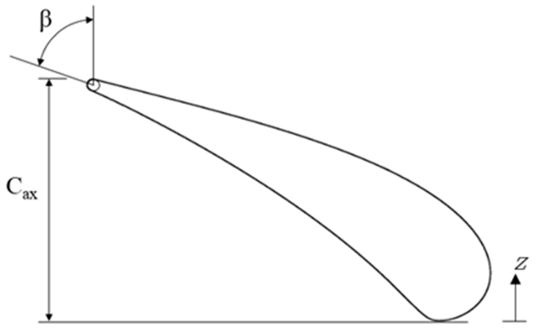
Figure 1. Nozzle guide vane profile.
Energies 14 05503 g001
Figure 2. Computational domain and surface mesh distribution.
Energies 14 05503 g002
Figure 3. Definitions of lean and sweep angle: (a) Circumferential view—Straight lean angle and compound lean angle; (b) Meridional view—Sweep angle.
Energies 14 05503 g003
Figure 4. Airfoil profiles of spanwise direction: (a) SL0 SP0; (b) SL0 SP10; (c) SL12 SP0; (d) CL12 SP0.
Energies 14 05503 g004
Figure 5. Swirl center location and measurement plane.
Energies 14 05503 g005
Figure 6. Comparison of surface pressure distribution of NGV.
Energies 14 05503 g006
Figure 7. Swirl vector at inlet plane: (a) Swirl at LE; (b) Swirl at passage center.
Energies 14 05503 g007
Figure 8. Comparison of stage efficiencies: (a) Straight lean; (b) Compound lean.
Energies 14 05503 g008
Figure 9. Variation of throat area and mass flow rate of the 3D NGVs: (a) Sweep with straight lean angle; (b) Straight lean with sweep angle; (c) Sweep with compound angle; (d) Compound lean with sweep angle.
Energies 14 05503 g009
Figure 10. Distributions of total pressure loss coefficient at NGV exit, z/Cax = 1.06 (rear view): (a) SL0 SP0; (b) SL0 SP10; (c) SL12 SP0; (d) SL12 SP10; (e) CL12 SP0; (f) CL12 SP10.
Energies 14 05503 g010
Figure 11. Comparison of circumferentially averaged static pressure, exit flow angle, and total pressure loss coefficient due to the straight lean, compound lean and sweep: (a) Static pressure with straight lean; (b) Flow angle with straight lean; (c) Total pressure loss with straight lean; (d) Static pressure with compound lean; (e) Flow angle with compound lean; (f) Total pressure loss with compound lean; (g) Static pressure with sweep; (h) Flow angle with sweep; (i) Total pressure loss with sweep.
Energies 14 05503 g011
Figure 12. Loading distribution of NGV loading at 10, 50 and 90% span heights.
Energies 14 05503 g012
Figure 13. Comparison of NGV loading due to the straight lean angle: (a) Span height 10%; (b) Span height 90%.
Energies 14 05503 g013
Figure 14. Comparison of NGV loading due to the compound lean angle: (a) Span height 10%; (b) Span height 90%.
Energies 14 05503 g014
Figure 15. Comparison of NGV loading due to sweep angle: (a) Span height 10%; (b) Span height 90%.
Energies 14 05503 g015
Figure 16. Comparison of NGV loading of the models with maximum efficiency (SL0 SP0 No swirl) and minimum efficiency (SL-12 SP-5 No swirl) model: (a) Span height 10%; (b) Span height 90%.
Energies 14 05503 g016
Figure 17. Comparison of circumferentially averaged mass flow rate (a), exit flow angle (b), and total pressure loss coefficient (c) due to the straight lean with sweep.
Energies 14 05503 g017
Figure 18. Comparison of circumferentially averaged mass flow rate (a), exit flow angle (b), and total pressure loss coefficient (c) due to the compound lean with sweep.
Energies 14 05503 g018
Figure 19. Comparison of NGV and Blade loading distributions of SL12 SP10 (a) and CL12 SP10 (b) models.
Energies 14 05503 g019
Figure 20. Comparison of vortex structure due to the swirl clocking−SL0 SP0 model (Baseline): (a) No swirl (front view); (b) SW@LE (front view); (c) SW@PC (front view); (d) No swirl (rear view); (e) SW@LE (rear view); (f) SW@PC (rear view).
Energies 14 05503 g020
Figure 21. Swirl clocking interaction with passage flow−the influence of straight lean angle: (a) SL12 SP0 No swirl; (b) SL12 SP0 SW@LE; (c) SL12 SP0 SW@PC; (d) SL−12 SP0 No swirl; (e) SL−12 SP0 SW@LE; (f) SL−12 SP0 SW@PC.
Energies 14 05503 g021
Figure 22. Comparison of vortex structure due to the swirl clocking−SL12 SP10 model: (a) SL12 SP10 No swirl; (b) SL12 SP10 SW@LE; (c) SL12 SP10 SW@PC.
Energies 14 05503 g022
Figure 23. Total pressure loss coefficient at vane exit, z/Cax = 1.06 (rear view): (a) SL0 SP0 SW@LE; (b) SL0 SP0 SW@PC; (c) SL12 SP0 SW@LE; (d) SL12 SP0 SW@PC; (e) CL12 SP0 SW@LE; (f) CL12 SP0 SW@PC; (g) SL0 SP10 SW@LE; (h) SL0 SP10 SW@PC.
Energies 14 05503 g023
Figure 24. Comparison of circumferentially averaged total pressure loss coefficients for passage 1 and 2.
Energies 14 05503 g024
Figure 25. Total pressure loss coefficient at the inlet and exit of blade (rear view), Baseline NGV: (a) Blade inlet, No swirl; (b) Blade inlet, SW@LE; (c) Blade inlet, SW@PC; (d) Blade exit, No swirl; (e) Blade exit, SW@LE; (f) Blade exit, SW@PC.
Energies 14 05503 g025
Figure 26. Total pressure loss coefficient at vane exit, z/Cax = 1.06 (rear view): (a) SL12 SP10 SW@LE; (b) SL12 SP10 SW@PC; (c) SL−12 SP10 SW@LE; (d) SL−12 SP10 SW@PC; (e) CL12 SP10 SW@LE; (f) CL12 SP10 SW@PC.
Energies 14 05503 g026
Figure 27. Total pressure loss coefficient at blade exit at z/Cax = 1.2 (rear view): (a) SL12 SP10 No swirl; (b) SL12 SP10 SW@LE; (c) SL12 SP10 SW@PC; (d) SL−12 SP10 No swirl; (e) SL−12 SP10 SW@LE; (f) SL−12 SP10 SW@PC; (g) CL12 SP10 No swirl; (h) CL12 SP10 SW@LE; (i) CL12 SP10 SW@PC.
Energies 14 05503 g027
Figure 28. Comparison of vortex structure due to the swirl clocking—Blade passage: (a) SL12 SP10 No swirl; (b) SL12 SP10 SW@LE; (c) SL12 SP10 SW@PC; (d) SL−12 SP10 No swirl; (e) SL−12 SP10 SW@LE; (f) SL−12 SP10 SW@PC; (g) CL12 SP10 No swirl; (h) CL12 SP10 SW@LE; (i) CL12 SP10 SW@PC.
Energies 14 05503 g028
Figure 29. Comparison of circumferentially averaged mass flow rate, exit flow angle, and total pressure loss coefficient due to swirl clocking: (a) SL12 SP0—NGV; (b) SL−12 SP0—NGV; (c) SL−12 SP10—NGV; (d) SL12 SP0—Blade; (e) SL−12 SP0—Blade; (f) SL−12 SP10—Blade.
Energies 14 05503 g029
Figure 30. Comparison of circumferentially averaged mass flow rate (a,d), exit flow angle (b,e), and total pressure loss coefficient (c,f) of the SL12 SP10 model due to swirl clocking.
Energies 14 05503 g030
Figure 31. Comparison of circumferentially averaged mass flow rate (a,d), exit flow angle (b,e), and total pressure loss coefficient (c,f) of the CL12 SP10 and CL−12 SP10 model due to swirl clocking.
Energies 14 05503 g031
Table 1. NGV geometric parameters and boundary conditions at 50% span height.
ParametersUnitNGVBlade
Airfoil count-3671
Axial chord, Caxmm123.6113.2
Exit metal angle, β°71.256.5
Tip clearancemm-2.2
Inlet total pressureBar22-
Inlet total temperatureK1873-
Stage pressure ratio, p01/p02-1.86-
Exit Mach number, M2-0.77-
Inlet Reynolds number, ReCax-1.32 × 10⁶-
Span height to axial chord, Hspan/Cax-1.432.69
Table 2. Lean and sweep angle range.
ParameterAbbreviationAngle Range
Straight lean angle (εs)SL−12°, −6°, 0°, +6°, +12°
Compound lean angle (εc)CL−12°, −6°, 0°, +6°, +12°
Sweep angle (γ)SP−5°, 0°, +5°, +10°
Table 3. 3D NGV geometry combination matrix.
Straight Lean (°)Sweep (°)Swirl
−12, −6, 0, 6, 12−5,0,5,10No swirl, swirl at LE, swirl at passage center
Compound Lean (°)Sweep (°)Swirl
−12, −6, 0, 6, 12−5,0,5,10No swirl, swirl at LE, swirl at passage center
Table 4. Highest stage performance models at proposed swirl clocking.
Swirl Clocking
Type of ModelNo SwirlSwirl @LESwirl @Passage Center
Straight Lean with SweepSL12 SP10SP-12 SP10SL12SP10
Compound Lean with SweepCL12 SP10CL12 SP10CL12 SP10
Publisher’s Note: MDPI stays neutral with regard to jurisdictional claims in published maps and institutional affiliations.

