Modeling and Control Design Based on Petri Nets Tool for a Serial Three-Phase Five-Level Multicellular Inverter Used as a Shunt Active Power Filter

Abstract

In this work, we represent a shunt active power filter (SAPF) based on a serial three-phase flying capacitor multilevel inverter (FCMI) controlled by a Petri Nets representation (PNs). This structure is chosen for its significant performances. In fact, the use of the FCMI within the SAPF makes it possible to increase the apparent switching frequency of the structure in order to reduce the value then the volume and weight of the inductance of the output filter. Besides, the FCMI allows the synthesis of a high-voltage signal using low-voltage semiconductor components. Therefore, improving the reliability of this structure leads to the improvement of the dynamics of the SAPF. This paper deals with a new control methodology based on PNs to regulate the flying capacitor voltages and the reference currents issued by the instantaneous active and reactive power theory. Compared to a conventional SAPF composed by a classical two-level inverter and controlled by a simple PWM control, simulation results demonstrate that our proposed control enhances the dynamic system and the power quality by reducing the total harmonic distortion (THD) satisfying the limits of IEEE standards.

1. Introduction

In recent years, the field of power electronics has seen a notable development mainly due to industrial applications using electrical systems [1,2,3]. However, every revolution comes with its benefits and drawbacks. In fact, any load based on power electronics devices has a so-called “nonlinear” behavior [4] because they create significant disturbances which degrade the optimal functioning of the installation and its overall efficiency, this also causes current deformation and creates additional losses and heating in the electrical equipments. In this context, three-phase nonlinear loads [5] lead, on the one hand, to a regular increase in the harmonic rate by producing harmonic currents whose frequencies are integer multiples of the fundamental frequency. By the other hand, they cause current imbalance and high consumption of reactive power. We can find these disturbance problems mainly in the industrial environment, in hospitals or others (control of rotating machines by inverters or rectifiers) [6,7]. To reduce the THD of currents delivered by these equipments and to ensure the performance of the dynamical system [8], power electronics have undergone significant technological development [9,10]. Those that best meet industrial constraints today are the parallel active filters. Thus, active filtering tends to cancel out harmonic currents by injecting signals with identical amplitudes but in phase opposition into the disturbing source, this one becomes sinusoidal after filtering. Indeed, a measurement of the nonlinear load current makes it possible to know the harmonic current to supply. The author of [11,12] explains the working principle of the active filters in depth. He reports several regulatory structures in his works, including an improved version of the RST, the latter demonstrates the limits of application of the classical RST. Several studies of SAPFs based on conventional inverters having a switching frequency between 12 and 16 kHz and consisting of two voltage level topology associated to a first-order output filter have been carried out; we note that this structure is expensive and very difficult to design. In contrast, the control of this structure is very easy to implement. The second structure represented in [13], which is based on the same conventional inverter associated, in this case, with an LCL output filter, is very easy to carry out but difficult to control. However, some scientific obstacles remain and need to be raised such as the hybrid control of hybrid dynamical systems (HDS) explicitly and simultaneously involving continuous and discrete behaviors. With a reduced number of switching inputs and a large number of variable states [14,15], these systems contribute to the improvement of the filtering function. The performance of these systems was demonstrated for a 4-cell inverter connected to an inductive load. Introduced in the 1980s and 1990s in [16], this structure constitutes a new solution: it consists of the design of new conversion architectures from the serial association of several switching cells. These associations allow the reduction of the constraints on switches providing multilevel output voltages with better quality compared to traditional architectures. The output signal is characterized by optimal spectral quality noted from the importance of the apparent switching frequency which increases to the value of the frequency of switching multiplied by the number of cells. These combinations of switching cells are made from energy storage elements which are floating capacitors. Their energy management is carried out according to the different states of each association so that their voltages remain always balanced around a fraction of the input voltage. This is ensured by following the principle of direct torque control (DTC) which was patented in [17]. This control is based on the principle of hysteresis control. It was initially reserved for asynchronous machines, then, advanced studies allow to use it for synchronous machines. The method of Pulse Width Modulation (PWM) is an extension of the DTC concept [18,19]. It is a conventional method associated with multicellular converters. The most used strategy is Phase Shifted modulation (PS) based on the PWM principle. Indeed, the regular phase shift between the control signals allows to increase the apparent frequency of the output voltage. This allows, therefore, to repel the harmonics of the output voltage, thus reducing the constraints related to the sizing of the output filter. Several works have been carried out for the development of the serial multicellular converters. Then, the authors of [20,21,22] have developed these structures and found adequate control strategies considering that this type of converters requires an in-depth study, especially with regard to the charges and discharges of floating capacitors [1,23,24]. The works of Guillaume Gateau led to two essential problems characterizing this type of converters, which are the saturation of the controls and the controllability of the floating voltages. Based on these principles, many recent studies have been treated. Compared to the traditional voltage source converters, the authors of [25,26] give an increasing attention to both of serial and parallel multicellular structures owing to their ability to synthesize signals with a better harmonic analysis. They focused their studies on observability and control based on sliding mode techniques represented in [27]. Recently, the authors in References [28,29] applied a control strategy based on Petri Nets representation to a multicellular converter. The main contribution of this strategy is the robust control of this type of inverter ensuring current regulation and voltage balancing. Appearing in 1962 as the subject of the doctoral thesis of Carl Adam Petri [30], PNs is considered as an alternative to automata models; it is a graphical and mathematical modeling language used as an approach for the description and the verification of the dynamical behavior of distributed Discrete Event Systems (DES) [3,31]. In this context, the authors in References [32,33] provide a viewpoint of the development of the field of DES. Furthermore, a control strategy based on two PNs representation is proposed to regulate simultaneously the capacitor voltages and the output current. To make sufficient conditions of control, a stability analysis is treated using Lyapunov method [34]. The main objective of using the FCMI within the SAPF is to increase the apparent switching frequency of the structure in order to give the possibility of reducing the value and consequently the volume, weight,.. of the inductance of the output filter. However, a second advantage of this structure is that the voltage applied to the power electronics components is lower than the overall voltage, which increases the operational reliability of the active filter. Note that increasing the number of components, compared to a conventional structure, reduces the overall reliability of the structure. Many active filter solutions for the depollution of electrical grids have been already proposed in the literature. In this paper, a PNs-based controller is applied to a multicell inverter for an active filter operation based on the principle of current reference. In fact, our SAPF structure based on an FCMI associated with a first-order output filter is not discussed in the literature; it has much fewer constraints, and the results presented here show the efficiency of the chosen algorithm in terms of robustness and stability. The remainder of this paper is structured as follows. First, the general model of our system is established. Then, SAPF is explained and the five-level FCMI is briefly described. Then, the control design based on PNs representation for an FCMI is presented along with Lyaponov analysis proofs. Afterwards, we give some simulation results to illustrate the validity of our proposed algorithm. Finally, some concluding remarks are given.

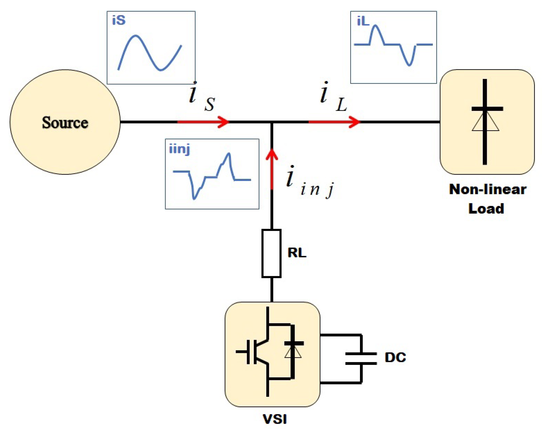
2. General Description of a Shunt Active Power Filter

As agreed, SAPFs have been introduced as a way to surmount the power quality problems caused by nonlinear and unbalanced loads. In fact, they identify and inject the disturbed currents with phase opposite towards the grid. The SAPFs attenuate a wide range of harmonics, and the filtering quality depends mainly on the performance of the chosen control. Figure 1 represents the global system: a three-phase network supplying three-phase nonlinear load and a filter mounted in parallel.

Therefore, an SAPF is basically made up of two parts: a power circuit constituted by a voltage source inverter (VSI) including a DC capacitive storage element, and an output passive filter (RL) permitting the VSI to connect to the grid. A control circuit is employed for the DC voltage regulation and for the VSI to ensure the injection of the currents into the network. This circuit is usually consisted of a disturbed current identification method we use the instantaneous, real and imaginary power method which is a well-established compensation technique [35]. The circuit also contains controllers based on the PWM-VSI method, which is used for controlling the switches. The importance of output filter is in preventing the components that are caused by the switching frequency from spreading into the grid without degrading the SAPF dynamics. By conclusion, the principle of the shunt active power filter is to produce harmonic currents equal in magnitude but opposite in-phase to those harmonics that are present in the grid following this equation: $i_{inj}=i_L-i_S$.

3. Modeling and Control of the SAPF

Nowadays, various configurations of SAPFs are studied and realized. Therefore, we can distinguish three tension structure configurations: single-phase filter, three-wire filter, and four-wire filter which is especially designed for the source current imbalance and to compensate the excessive harmonic current in the neutral. It is therefore an inverter connected to the grid via a passive L-R filter. It is mounted in parallel with the three-phase network and injects in real-time the harmonic components of the currents absorbed by the nonlinear loads connected to the network. Marketed inverters used for actual SAPF applications are almost the classical two level inverters. These ones show a switching frequency around 16 kHz. Further, at this frequency, the output filter is very heavy, voluminous, expensive, and very difficult to design.

Thus, our choice is based on a hybrid dynamical model with instantaneous values, known as a five-level FCMI because, on the one hand, it makes it possible to limit the voltage constraints undergone by the power switches: each component, in a blocked state, supports a smaller fraction of full DC bus voltage as the number of levels is high. On the other hand, the output voltage delivered shows interesting spectral qualities. Therefore, this model allows the study of the evolution of the different states in order to generate the polluted current and to balance the voltages of the flying capacitors. This topology includes p cells, and between each two cells we insert flying capacitors as continuous sources. Thus, an FCMI is composed by p-1 floating voltage sources; note that p is equal to n-1 with n is the level number of the corresponding structure. Each cell contains two complementary switches controlled by a binary function. The FCMI therefore requires careful control of the switches allowing it to eliminate certain harmonics.

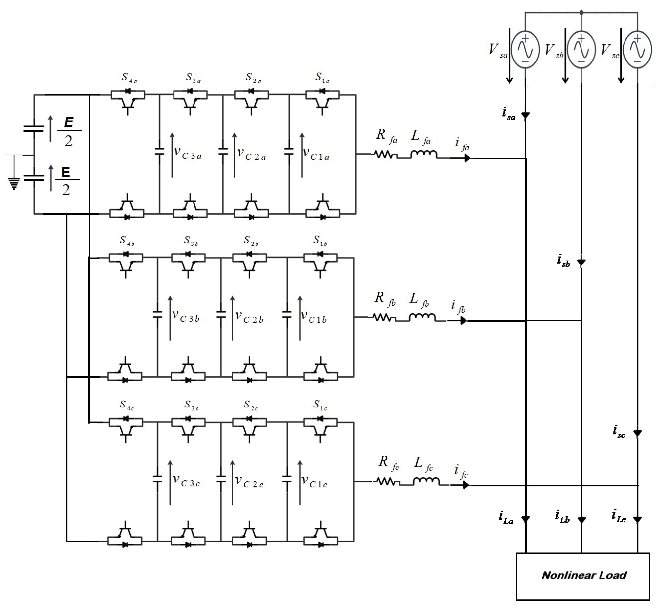
3.1. SAPF Modeling and Description

Figure 2 shows the power circuit of a three-phase SAPF based on three-phase four-level multicellular power inverter as previously described. In this system, considering an ideal grid, the FCMI injects an opposite current harmonic to make a sinusoidal grid-side current then obtains a unity power factor.

The current filter variations are given in the following equation:

$$\frac{d{i}_{f_k}}{dt}=\frac{(S_{1k}-S_{2k})}{L_{f_k}}{v}_{ck1}+\frac{(S_{2k}-S_{3k})}{L_{f_k}}{v}_{ck2}+\frac{(S_{3k}-S_{4k})}{L_{f_k}}{v}_{ck3}+\frac{(S_{4k}-\overline{S_{4k}})}{L_{f_k}}{V}_{dc}-\frac{R_{f_k}}{L_{f_k}}{i}_{f_k}-\frac{v_{s_k}}{L_{f_k}}$$

(1)

With $v_{s_k}$ being the supply voltage and $i_{f_k}$ being the output current which is equal to

$$i_{f_k}=i_{L_k}-i_{s_k}\mathrm{with}\mathrm{k}\in [\mathrm{a},\mathrm{b},\mathrm{c}]$$

A coupled state representation of three-phase SAPF with five-level MFCI is given as follows:

$$\left[\begin{array}{c}\dot{v_{ck1}}\\ \dot{v_{ck2}}\\ \dot{v_{ck3}}\\ \dot{i_{f_k}}\end{array}\right]=\left[\begin{array}{cccc}0& 0& 0& \frac{S_{2k}-S_{1k}}{C_1}\\ 0& 0& 0& \frac{S_{3k}-S_{2k}}{C_2}\\ 0& 0& 0& \frac{S_{4k}-S_{3k}}{C_3}\\ \frac{S_{1k}-S_{2k}}{L_{f_k}}& \frac{S_{2k}-S_{3k}}{L_{f_k}}& \frac{S_{3k}-S_{4k}}{L_{f_k}}& -\frac{R_{f_k}}{L_{f_k}}\end{array}\right]\times \left[\begin{array}{c}{v}_{ck1}\\ v_{ck2}\\ v_{ck3}\\ i_{f_k}\end{array}\right]+\left[\begin{array}{c}0\\ 0\\ 0\\ \frac{(S_{4k}-\overline{S_{4k}})V_{dc}}{L_{f_k}}-\frac{v_{s_k}}{L_{f_k}}\end{array}\right]$$

(2)

This model can be expressed in a compact form as

$$\dot{x}=A_{q_j}x+B_{q_j}$$

(3)

where the square matrix $A_{q_j}$∈$R^{4\times 4}$, $B_{q_j}$∈$R^{4\times 1}$, and x∈$R^{4\times 1}$ representing the state vector, $q_j$ represents the $2^p$ discrete variables. Each mode of operation is given by a set of possible switching combinations called (SDD) (Specific discontinuous driving) $q_j\in \left\{S_1,S_2,S_3,S_4\right\}$ with $j\in \left\{1\dots 7\right\}$.

In order to ensure normal operations, a balanced distribution of the floating voltages should be necessary guarantee as follows:

$$\left\{\begin{array}{c}V{c_{k_1}}^{\ast }=\frac{E}{4}\hfill \\ V{c_{k_2}}^{\ast }=\frac{E}{2}\hfill \\ V{c_{k_3}}^{\ast }=\frac{3E}{4}\hfill \end{array}\right.$$

(4)

With $V_{dc}$ is the DC source that should be equal to $\frac{E}{2}$ and E represents the input voltage.

Sizing of the DC Bus Voltage

The fundamental current delivered by the filter is given by

$$I_{f_1}=\frac{V_{f_1}-V_s}{\omega L_f}=\frac{V_{f_1}}{\omega L_f}(1-\frac{V_s}{\omega V_{f_1}})$$

(5)

With $V_s$ is the supply voltage and $V_{f_1}$ indicates the fundamental component of the output voltage of the SAPF and $L_f$ is its inductance.

The reactive energy delivered by the filter is

$$Q_f=3V_s{I}_{f_1}$$

(6)

Then,

$$Q_f=3V_s\frac{V_{f_1}}{\omega L_f}(1-\frac{V_s}{\omega V_{f_1}})$$

(7)

This allows the active filter to compensate reactive energy if and only if $V_{f_1}>V_s$.

The maximum reactive power is then obtained from the derivative of the reactive power with respect to the grid voltage $\frac{d{Q}_f}{d{V}_s}=0$, then

$$\frac{d{Q}_f}{d{V}_s}=\frac{3V_{f_1}}{\omega L_f}(1-\frac{2V_s}{\omega V_{f_1}})=0$$

(8)

As a result, the maximum compensation capacity of the active filter occurs at $V_{f_1}=2V_s$ and the maximum energy is the following:

$$d{Q}_{f_{max}}=\frac{3V_s}{\omega L_f}$$

(9)

$$V_s<V_{f_1}<2V_s$$

(10)

$$V_{f_1}\sqrt{2}=\frac{E}{2}$$

(11)

$$E=2\sqrt{2}{V}_{f_1}$$

(12)

$$\sqrt{2}{V}_s<E<2\sqrt{2}{V}_s$$

(13)

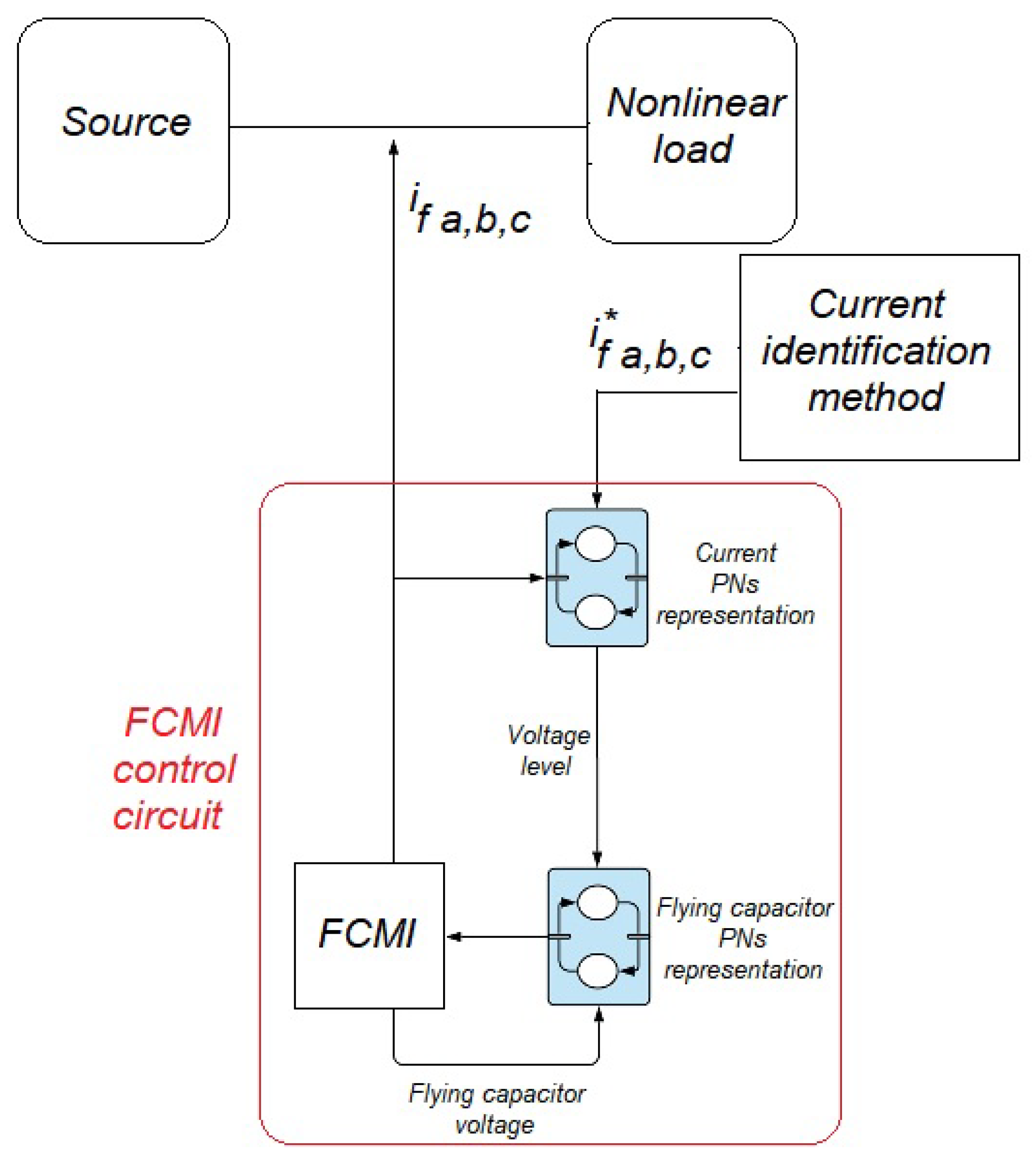
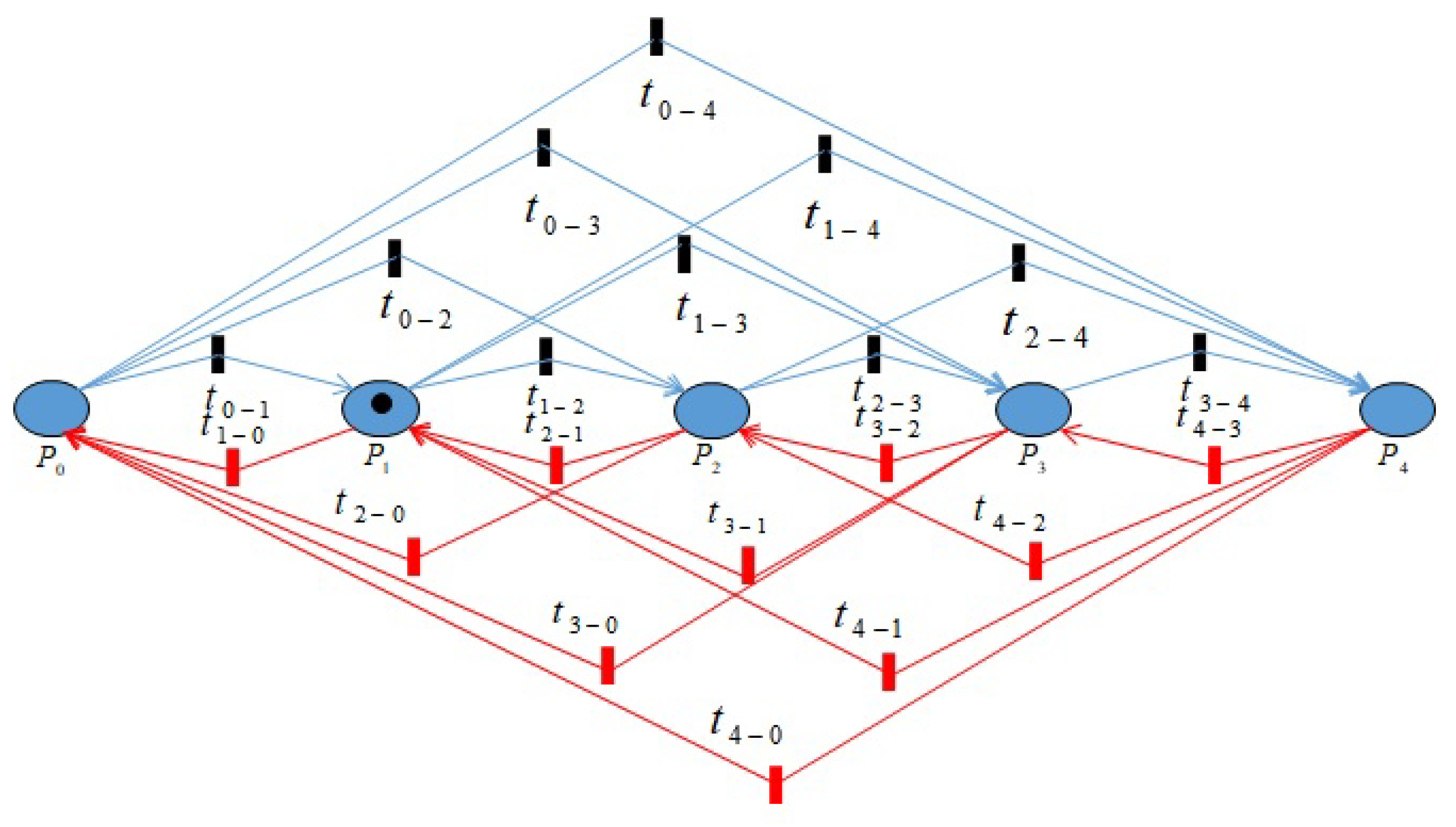
3.2. Hybrid Control Design Based on Petri Nets Modelization

Hybrid dynamical systems (HDS) result from the hierarchical organization of complex control or the interaction between discrete planning and continuous control algorithms.

To highlight the control of our chosen HDS, two cascaded PNs representations are proposed and developed. The first PNs allows the reference current regulation giving the required voltage level, while the second one ensures, by one side, the voltage level corresponding to the current regulation and the balance of the capacitor voltages by another side. Note that the reference current is determined by the instantaneous active and reactive method. The Figure 3 describes the regulation principle.

Note that the regulation algorithm is carried out while ensuring the development of the following points:

• SDD selection:
  The selection of the SDD must ensure simultaneously the output current regulation and the capacitor voltage regulation. The following control property make it possible to establish the conditions ensuring the convergence of current error and capacitor voltages errors to zero then we can determine the appropriate SDD that should be selected.

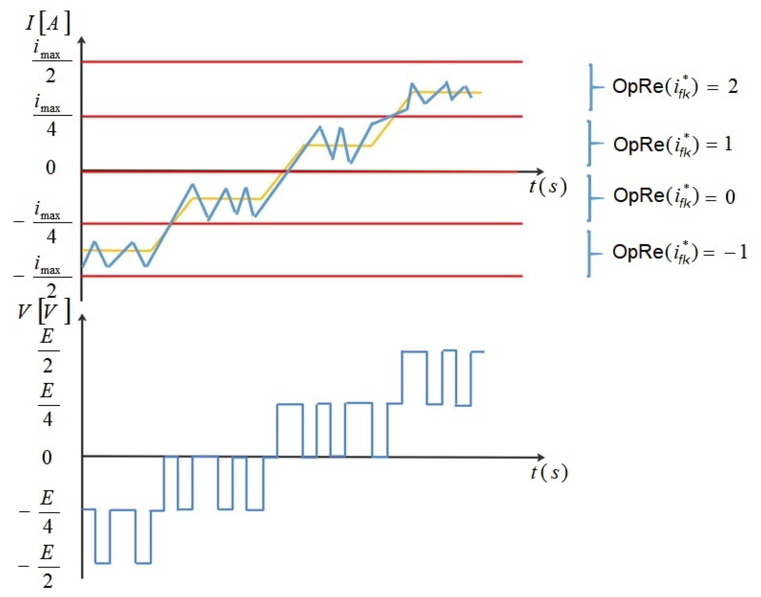
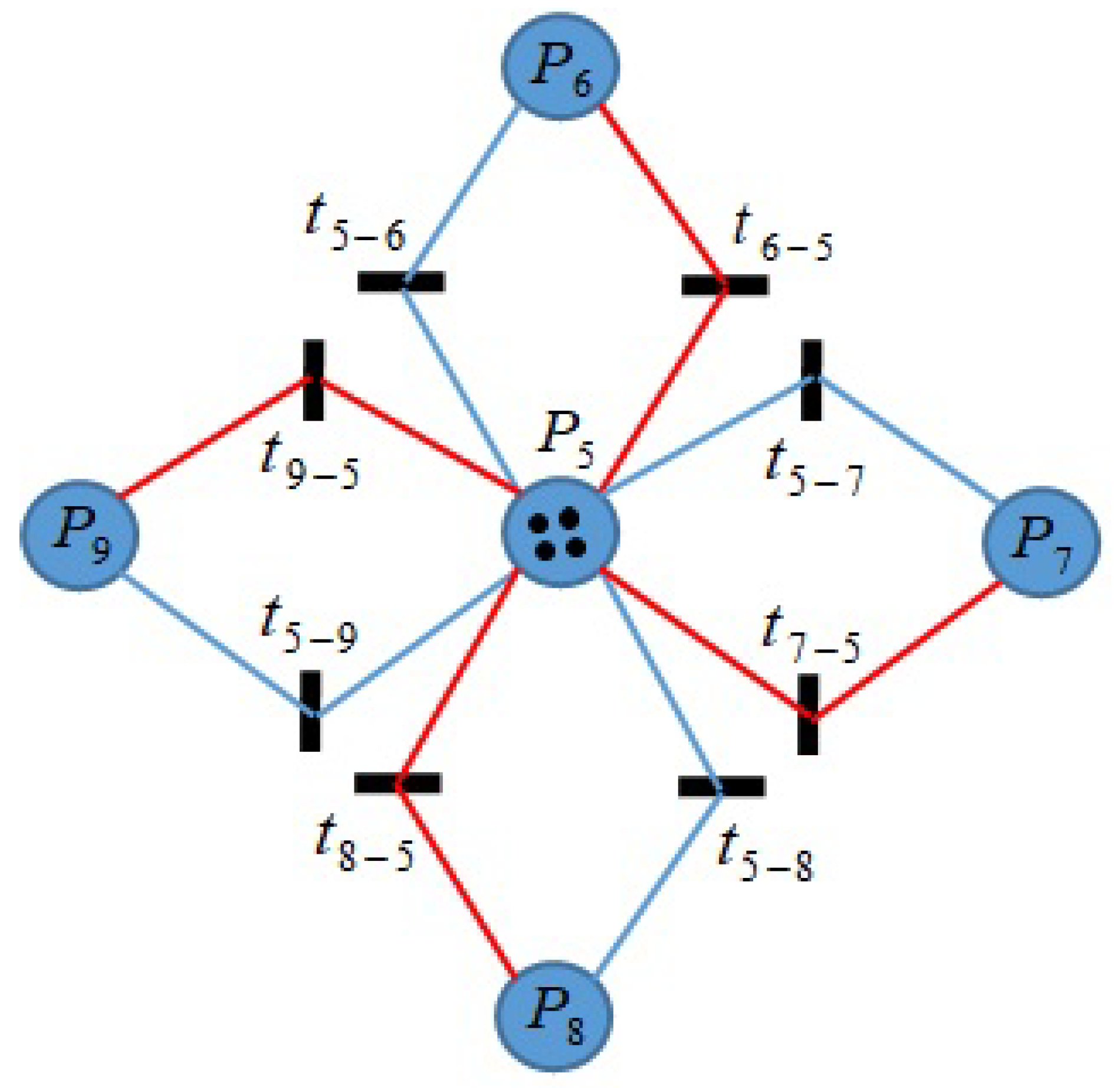
Proposition 1.

For any initial condition, there exits an SDD such that the capacitor voltages and the output current converge to their reference values.

Proof. 

Consider the Lyapunov function as follows:

$$V=\frac{1}{2}\sum _{j=1}^{n-2}{C}_j{e}_j^2+\frac{1}{2}L{e}_i^2$$

(14)

where $e_i=i_{fk}-i_{f_k}^{\ast }$ is the the output current error and $e_j=v_{cjk}-v_{cjk}^{\ast };j\in [1\dots n-2]$ is the capacitor voltage error. Taking the time derivative of Equation (14) for n = 5:

$$\dot{V}=i_{fk}·[e_1·(S_2-S_1)+e_2·(S_3-S_2)+e_3·(S_4-S_3)]+e_i·[(S_1-S_2)·v_{c1k}+$$

$$(S_2-S_3)·v_{c2k}+(S_3-S_4)·v_{c3k}+(S_4-\overline{S_4})·V_{dc}-R·i_{fk}-v_{sk}]$$

(15)

We aim to obtain $\dot{V}<0$ under the action of the SDDs. It can be noticed that for each discrete voltage level L there is at least one SDD holding $\dot{V}<0$.

Table 1. Evaluation of Equation (15) for each SDD.

SDD	${\dot{\mathit{V}}}_{{\mathit{q}}_{\mathit{i}}}$
$q_0$	${\dot{V}}_{q_0}=e_i\times \left(-V_{dc}-R\times i_{fk}-v_{sk}\right)$
$q_1$	${\dot{V}}_{q_1}=-e_1\times i_{fk}+e_i\times (v_{c1k}-V_{dc}$$-R\times i_{fk}-v_{sk})$
$q_2$	${\dot{V}}_{q_2}=(e_1-e_2)\times i_{fk}+e_i\times (-v_{c1k}+v_{c2k}$$-V_{dc}-R\times i_{fk}-v_{sk})$
$q_3$	${\dot{V}}_{q_3}=-e_2\times i_{fk}+e_i\times (v_{c2k}-V_{dc}$$-R\times i_{fk}-v_{sk})$
$q_4$	${\dot{V}}_{q_4}=(e_2-e_3)\times i_{fk}+e_i\times (-v_{c2k}+v_{c3k}$$-V_{dc}-R\times i_{fk}-v_{sk})$
$q_5$	${\dot{V}}_{q_5}=(-e_1+e_2-e_3)\times i_{fk}+e_i\times (v_{c1k}$$-v_{c2k}+v_{c3k}-V_{dc}-R\times i_{fk}-v_{sk})$
$q_6$	${\dot{V}}_{q_6}=(e_1-e_3)\times i_{fk}+e_i\times (-v_{c1k}+v_{c3k}$$-V_{dc}-R\times i_{fk}-v_{sk})$
$q_7$	${\dot{V}}_{q_7}=-e_3\times i_{fk}+e_i\times (v_{c3k}-V_{dc}$$-R\times i_{fk}-v_{sk})$
$q_8$	${\dot{V}}_{q_8}=e_3\times i_{fk}+e_i\times (-v_{c3k}+V_{dc}-v_{sk}$$-R\times i_{fk})$
$q_9$	${\dot{V}}_{q_9}=(-e_1+e_3)\times i_{fk}+e_i\times (v_{c1k}-v_{c3k}$$+V_{dc}-v_{sk}-R\times i_{fk})$
$q_{10}$	${\dot{V}}_{q_{10}}=(e_1-e_2+e_3)\times i_{fk}+e_i\times (-v_{c1k}$$+v_{c2k}-v_{c3k}+V_{dc}-v_{sk}-R\times i_{fk})$
$q_{11}$	${\dot{V}}_{q_{11}}=(-e_2+e_3)\times i_{fk}+e_i\times (v_{c2k}-v_{c3k}$$+V_{dc}-v_{sk}-R\times i_{fk})$
$q_{12}$	${\dot{V}}_{q_{12}}=e_2\times i_{fk}+e_i\times (-v_{c2k}+V_{dc}-v_{sk}$$-R\times i_{fk})$
$q_{13}$	${\dot{V}}_{q_{13}}=(-e_1+e_2)\times i_{fk}+e_i\times (v_{c1k}-v_{c2k}$$+V_{dc}-v_{sk}-R\times i_{fk})$
$q_{14}$	${\dot{V}}_{q_{14}}=e_1\times i_{fk}+e_i\times (-v_{c1k}+V_{dc}-v_{sk}$$-R\times i_{fk})$
$q_{15}$	${\dot{V}}_{q_{15}}=e_i\times (V_{dc}-v_{sk}-R\times i_{fk})$

summarizes the equations obtained from 15. □

• First Petri Nets representation:
  The objective of this PNs representation is to select the appropriate voltage level to reach the current reference. As shown in Figure 4, the behavior of the output current follows the corresponding voltage level for a five-level FCMI, with imax = $\frac{V_{dc}-V_{smax}}{2\ast R}$. With $V_{smax}$ is the maximum supply voltage.

Figure 4. Petri Nets representation for output current regulation.

Figure 4. Petri Nets representation for output current regulation.

The places of this PNs representation are defined in

Table 2. Designation of the places defining the PNs representation of the output current control.

Place	Designation
$P_0$	Level $L=-2$, corresponding to the minimum voltage $-\frac{E}{2}V$
$P_1$	Level $L=-1$, corresponding to the voltage $-\frac{E}{4}V$
$P_2$	Level $L=0$, corresponding to the voltage $0 V$
$P_3$	Level $L=1$, corresponding to the voltage $\frac{E}{4}V$
$P_4$	Level $L=2$, corresponding to the maximum voltage $\frac{E}{2}V$

.

The token is moved to the place corresponding to the required voltage level which is obtained by defining at first an operating region $OpRe\left(i^{\ast }\right)$ as follows:

$$\frac{w-1}{n-1}\times i_{max}\le i_{fk}^{\ast }\le \frac{w}{n-1}\times i_{max}\Rightarrow OpRe\left(i_{fk}^{\ast }\right)=w$$

(16)

where $w\in [-1;2]$.

Then, the required voltage level $m\in [1\dots 4]$ for the output current regulation of a 5-level FCMI is

$$L_m\left(i_{fk}^{\ast }\right)=\left\{\begin{array}{c}OpRe\left(i_{fk}^{\ast }\right)if{i}_{fk}<i_{fk}^{\ast }\hfill \\ L_{m-1}if{i}_{fk}=i_{fk}^{\ast }\hfill \\ OpRe\left(i_{fk}^{\ast }\right)-1if{i}_{fk}>i_{fk}^{\ast }\hfill \end{array}\right.$$

(17)

Figure 5 describes the behavior of the control law.

Finally, the rules that fire the transitions to transfer a token from a place to another are summarized in

Table 3. Firing transition rules and output FCMI voltage level obtained.

Transition	Transition Rule	Reached Level
$t_{0-1}$	$(OpRe\left(i_{fk}^{\ast }\right)=-1)\wedge (i_{fk}\le i_{fk}^{\ast })$	−1
$t_{1-0}$	$(OpRe\left(i_{fk}^{\ast }\right)=-1)\wedge (i_{fk}\ge i_{fk}^{\ast })$	−2
$t_{0-2}$	$(OpRe\left(i_{fk}^{\ast }\right)=0)\wedge (i_{fk}\le i_{fk}^{\ast })$	0
$t_{2-0}$	$(OpRe\left(i_{fk}^{\ast }\right)=-1)\wedge (i_{fk}\ge i_{fk}^{\ast })$	−2
$t_{0-3}$	$(OpRe\left(i_{fk}^{\ast }\right)=1)\wedge (i_{fk}\le i_{fk}^{\ast })$	1
$t_{3-0}$	$(OpRe\left(i_{fk}^{\ast }\right)=-1)\wedge (i_{fk}\ge i_{fk}^{\ast })$	−2
$t_{0-4}$	$(OpRe\left(i_{fk}^{\ast }\right)=2)\wedge (i_{fk}\le i_{fk}^{\ast })$	2
$t_{4-0}$	$(OpRe\left(i_{fk}^{\ast }\right)=-1)\wedge (i_{fk}\ge i_{fk}^{\ast })$	−2
$t_{1-2}$	$(OpRe\left(i_{fk}^{\ast }\right)=0)\wedge (i_{fk}\le i_{fk}^{\ast })$	0
$t_{2-1}$	$(OpRe\left(i_{fk}^{\ast }\right)=0)\wedge (i_{fk}\ge i_{fk}^{\ast })$	−1
$t_{1-3}$	$(OpRe\left(i_{fk}^{\ast }\right)=1)\wedge (i_{fk}\le i_{fk}^{\ast })$	1
$t_{3-1}$	$(OpRe\left(i_{fk}^{\ast }\right)=0)\wedge (i_{fk}\ge i_{fk}^{\ast })$	−1
$t_{1-4}$	$(OpRe\left(i_{fk}^{\ast }\right)=2)\wedge (i_{fk}\le i_{fk}^{\ast })$	2
$t_{4-1}$	$(OpRe\left(i_{fk}^{\ast }\right)=0)\wedge (i_{fk}\ge i_{fk}^{\ast })$	−1
$t_{2-3}$	$(OpRe\left(i_{fk}^{\ast }\right)=1)\wedge (i_{fk}\le i_{fk}^{\ast })$	1
$t_{3-2}$	$(OpRe\left(i_{fk}^{\ast }\right)=1)\wedge (i_{fk}\ge i_{fk}^{\ast })$	0
$t_{2-4}$	$(OpRe\left(i_{fk}^{\ast }\right)=2)\wedge (i_{fk}\le i_{fk}^{\ast })$	2
$t_{4-2}$	$(OpRe\left(i_{fk}^{\ast }\right)=1)\wedge (i_{fk}\ge i_{fk}^{\ast })$	0
$t_{3-4}$	$(OpRe\left(i_{fk}^{\ast }\right)=2)\wedge (i_{fk}\le i_{fk}^{\ast })$	2
$t_{4-3}$	$(OpRe\left(i_{fk}^{\ast }\right)=2)\wedge (i_{fk}\ge i_{fk}^{\ast })$	1

.

• Second Petri Nets representation:
  Considering the required voltage level determined by the first PNs, a second PNs representation was established to select the SDD to ensure simultaneously the pursuit of the reference current and the balance of the capacitor voltages. Table 4 shows the conditions in order to choose the equivalent SDD. The symbol (–) represents when no change is taking place and $e_j\to 0$ represents when the error voltage of the jth capacitor tends to zero.

Table 4. FMCI capacitor voltage convergence.

SDD	${\mathit{e}}_1$ → 0	${\mathit{e}}_2$ → 0	${\mathit{e}}_3$ → 0	${\mathit{i}}_{\mathit{fk}}$
$q_0$	–	–	–	$i_{fk}>0$
	–	–	–	$i_{fk}<0$
$q_1$	$e_1>0$	–	–	$i_{fk}>0$
	$e_1<0$	–	–	$i_{fk}<0$
$q_2$	$e_1<0$	$e_2>0$	–	$i_{fk}>0$
	$e_1>0$	$e_2<0$	–	$i_{fk}<0$
$q_3$	–	$e_2>0$	–	$i_{fk}>0$
	–	$e_2<0$	–	$i_{fk}<0$
$q_4$	–	$e_2<0$	$e_3>0$	$i_{fk}>0$
	–	$e_2>0$	$e_3<0$	$i_{fk}<0$
$q_5$	$e_1>0$	$e_2<0$	$e_3>0$	$i_{fk}>0$
	$e_1<0$	$e_2>0$	$e_3<0$	$i_{fk}<0$
$q_6$	$e_1<0$	–	$e_3>0$	$i_{fk}>0$
	$e_1>0$	–	$e_3<0$	$i_{fk}<0$
$q_7$	–	–	$e_3>0$	$i_{fk}>0$
	–	–	$e_3<0$	$i_{fk}<0$
$q_8$	–	–	$e_3<0$	$i_{fk}>0$
	–	–	$e_3>0$	$i_{fk}<0$
$q_9$	$e_1>0$	–	$e_3<0$	$i_{fk}>0$
	$e_1<0$	–	$e_3>0$	$i_{fk}<0$
$q_{10}$	$e_1<0$	$e_2>0$	$e_3<0$	$i_{fk}>0$
	$e_1>0$	$e_2<0$	$e_3>0$	$i_{fk}<0$
$q_{11}$	–	$e_2>0$	$e_3<0$	$i_{fk}>0$
	–	$e_2<0$	$e_3>0$	$i_{fk}<0$
$q_{12}$	–	$e_2>0$	–	$i_{fk}>0$
	–	$e_2<0$	–	$i_{fk}<0$
$q_{13}$	$e_1>0$	$e_2<0$	–	$i_{fk}>0$
	$e_1<0$	$e_2>0$	–	$i_{fk}<0$
$q_{14}$	$e_1>0$	–	–	$i_{fk}>0$
	$e_1<0$	–	–	$i_{fk}<0$
$q_{15}$	–	–	–	$i_{fk}>0$
	–	–	–	$i_{fk}<0$

Table 4. FMCI capacitor voltage convergence.

SDD	${\mathit{e}}_1$ → 0	${\mathit{e}}_2$ → 0	${\mathit{e}}_3$ → 0	${\mathit{i}}_{\mathit{fk}}$
$q_0$	–	–	–	$i_{fk}>0$
	–	–	–	$i_{fk}<0$
$q_1$	$e_1>0$	–	–	$i_{fk}>0$
	$e_1<0$	–	–	$i_{fk}<0$
$q_2$	$e_1<0$	$e_2>0$	–	$i_{fk}>0$
	$e_1>0$	$e_2<0$	–	$i_{fk}<0$
$q_3$	–	$e_2>0$	–	$i_{fk}>0$
	–	$e_2<0$	–	$i_{fk}<0$
$q_4$	–	$e_2<0$	$e_3>0$	$i_{fk}>0$
	–	$e_2>0$	$e_3<0$	$i_{fk}<0$
$q_5$	$e_1>0$	$e_2<0$	$e_3>0$	$i_{fk}>0$
	$e_1<0$	$e_2>0$	$e_3<0$	$i_{fk}<0$
$q_6$	$e_1<0$	–	$e_3>0$	$i_{fk}>0$
	$e_1>0$	–	$e_3<0$	$i_{fk}<0$
$q_7$	–	–	$e_3>0$	$i_{fk}>0$
	–	–	$e_3<0$	$i_{fk}<0$
$q_8$	–	–	$e_3<0$	$i_{fk}>0$
	–	–	$e_3>0$	$i_{fk}<0$
$q_9$	$e_1>0$	–	$e_3<0$	$i_{fk}>0$
	$e_1<0$	–	$e_3>0$	$i_{fk}<0$
$q_{10}$	$e_1<0$	$e_2>0$	$e_3<0$	$i_{fk}>0$
	$e_1>0$	$e_2<0$	$e_3>0$	$i_{fk}<0$
$q_{11}$	–	$e_2>0$	$e_3<0$	$i_{fk}>0$
	–	$e_2<0$	$e_3>0$	$i_{fk}<0$
$q_{12}$	–	$e_2>0$	–	$i_{fk}>0$
	–	$e_2<0$	–	$i_{fk}<0$
$q_{13}$	$e_1>0$	$e_2<0$	–	$i_{fk}>0$
	$e_1<0$	$e_2>0$	–	$i_{fk}<0$
$q_{14}$	$e_1>0$	–	–	$i_{fk}>0$
	$e_1<0$	–	–	$i_{fk}<0$
$q_{15}$	–	–	–	$i_{fk}>0$
	–	–	–	$i_{fk}<0$

The places of the second PNs representation are defined in

Table 5. Designation of the places defining the PNs representation of the flying capacitor control.

Place	Designation
$P_5$	Initial state
$P_6$	Closing of the first switch
$P_7$	Closing of the second switch
$P_8$	Closing of the third switch
$P_9$	Closing of the fourth switch

.

The movement of the token from one place to another is described according to the following procedure:

–

Step 1: Choose the subset that contains all SDDs of the desired voltage level L.

–

Step 2: Select an SDD that reduces the error in the capacitor voltages as described in Table 4.

–

Step 3: In the case where exists more than one SDD, the one that reduces the greater number of voltage errors will be selected.

–

Step 4: The SDD which allows the reduction of errors by increasing the voltages of the capacitors will be chosen among the rest of the existing choices.

Figure 6 represents the Petri diagram which describes the algorithm defined by the procedure previously explained, and

Table 6. This is a table caption. Tables should be placed in the main text near to the first time they are cited.

Transition	Transition Rule
$t_{5-6}$	$((L=-1)\wedge \left(e_1^{+}\right)\vee (L=0)\wedge (e_2^{+}\vee (e_1^{+}\wedge e_2^{-}\wedge e_3^{+})\vee (e_1^{+}\wedge e_3^{-}))$
	$\vee (L=1)\wedge (e_3^{+}\vee (e_2^{+}\wedge e_3^{-})\vee (e_1^{+}\wedge e_2^{-}))\vee (L=2))\wedge (i_{fk}>0)$
$t_{5-7}$	$((L=-1)\wedge (e_1^{-}\wedge e_2^{+})\vee (L=0)\wedge (e_2^{+}\vee (e_1^{-}\wedge e_3^{+})\vee (e_1^{-}\wedge e_2^{+}\wedge e_3^{-}))$
	$\vee (L=1)\wedge (e_3^{+}\vee (e_2^{+}\wedge e_3^{-})\vee e_1^{+})\vee (L=2))\wedge (i_{fk}>0)$
$t_{5-8}$	$((L=-1)\wedge (e_2^{-}\wedge e_3^{+})\vee (L=0)\wedge ((e_1^{+}\wedge e_2^{-}\wedge e_3^{+})\vee (e_1^{-}\wedge e_3^{+})\vee e_2^{+})$
	$\vee (L=1)\wedge (e_3^{+}\vee (e_1^{+}\wedge e_2^{-})\vee e_1^{+})\vee (L=2))\wedge (i_{fk}>0)$
$t_{5-9}$	$((L=-1)\wedge \left(e_3^{-}\right)\vee (L=0)\wedge ((e_1^{+}\wedge e_3^{-})\vee (e_1^{-}\wedge e_2^{+}\wedge e_3^{-})\vee e_2^{+})$
	$\vee (L=1)\wedge ((e_2^{+}\wedge e_3^{-})\vee (e_1^{+}\wedge e_2^{-})\vee e_1^{+})\vee (L=2))\wedge (i_{fk}>0)$

summarizes the laws of the transitions chosen for this Petri networks when the output current is positive, note that $e_j^{+}\equiv e_j>0$ and $e_j^{-}\equiv e_j<0$ for j = 1, 2, 3.

Finally, the global system composed by a SAPF based on three-phase 5-level FCMI controlled by a PNs representation is developed.

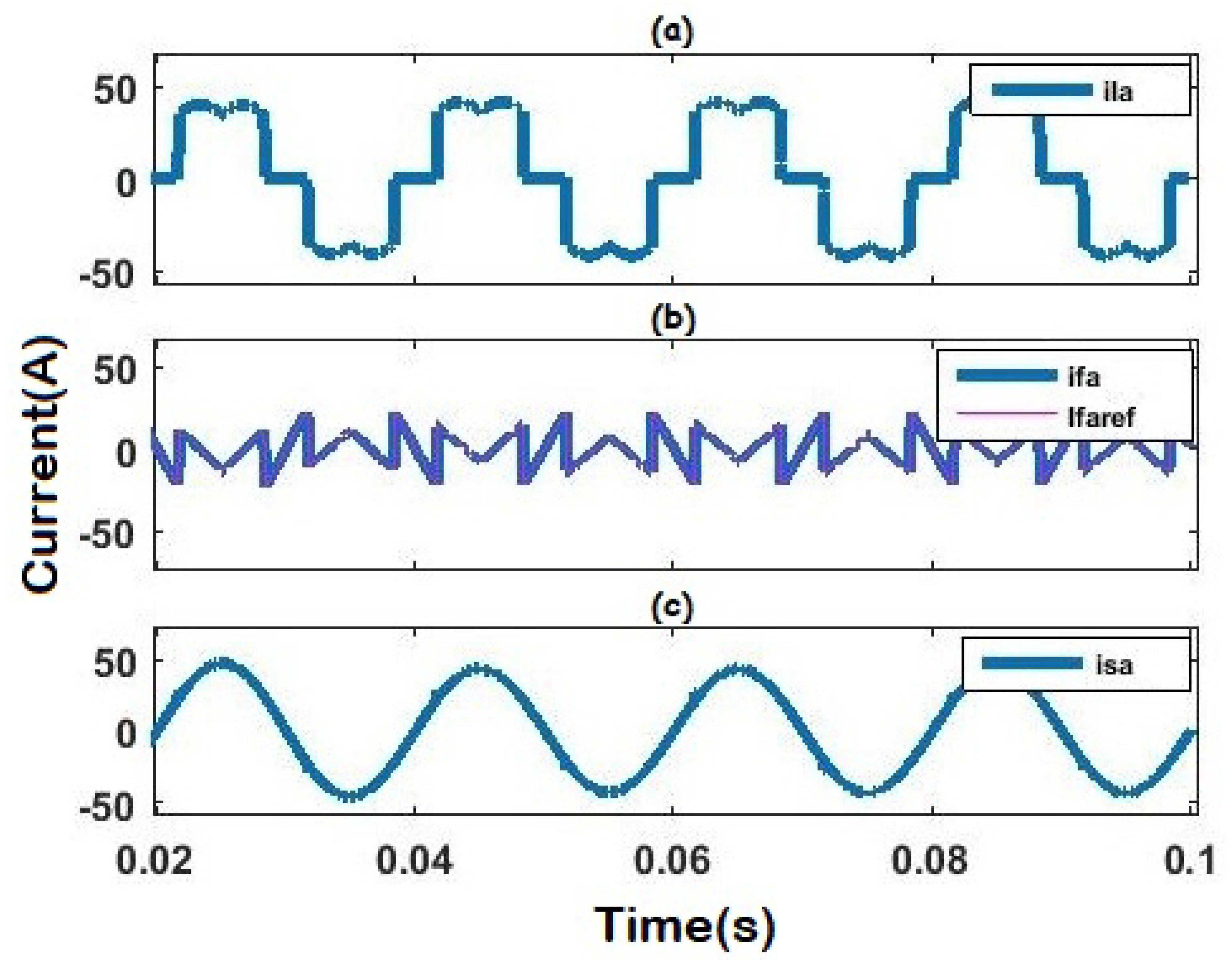
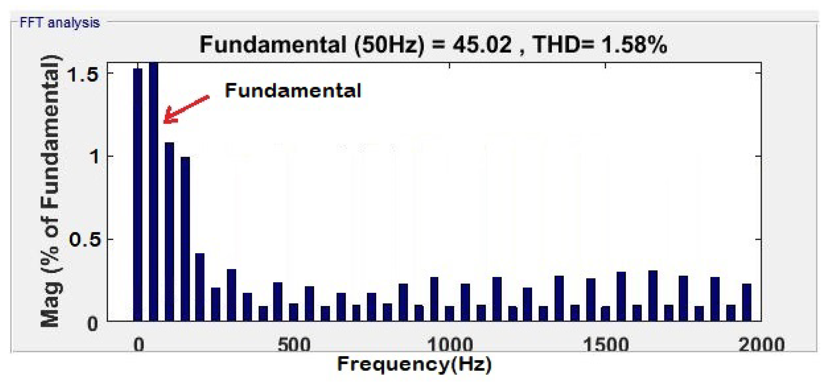
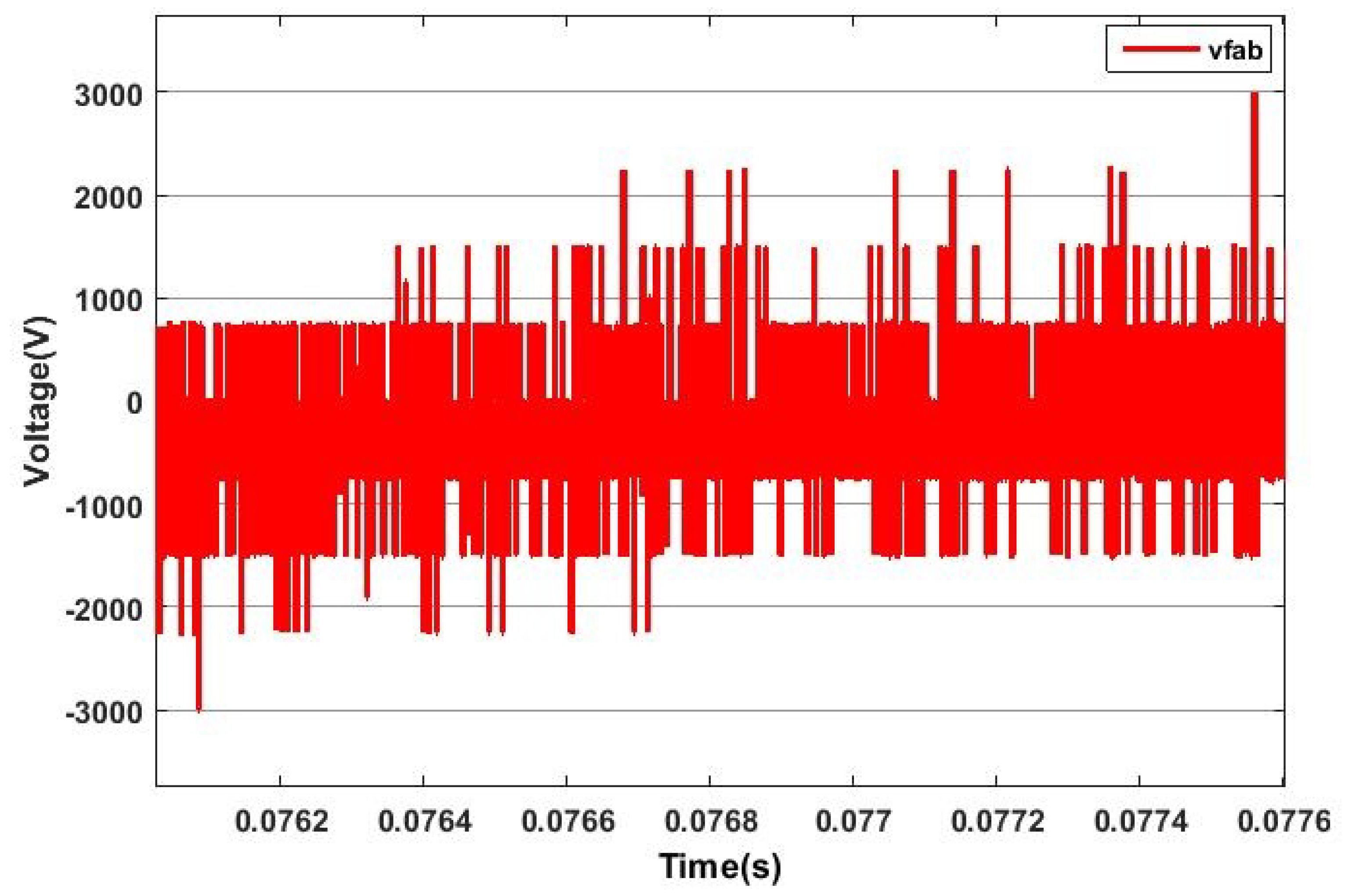
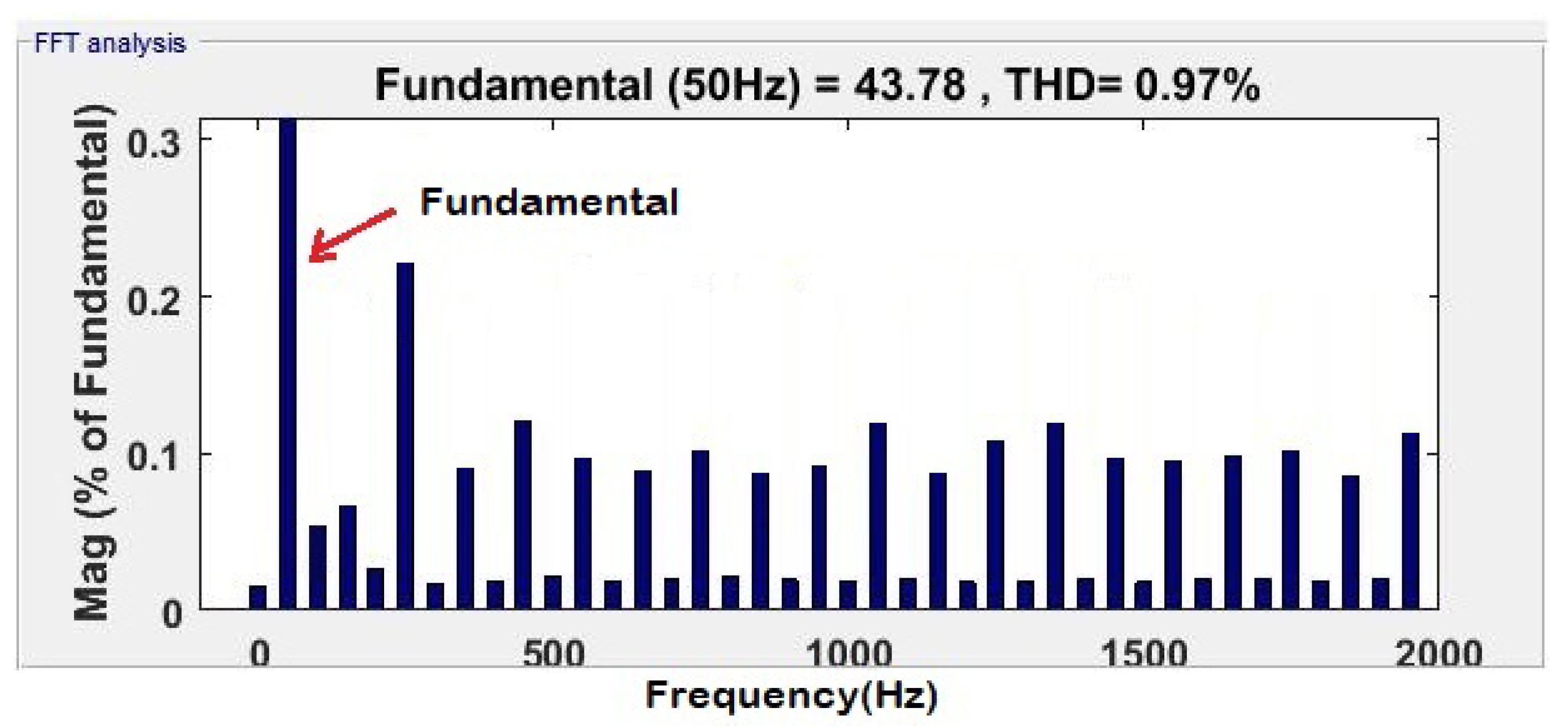
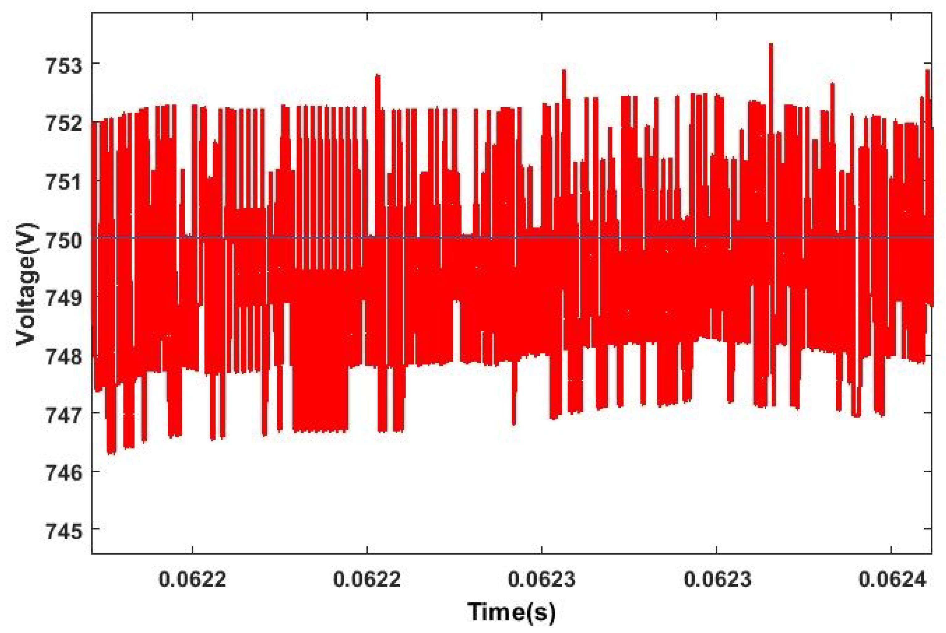
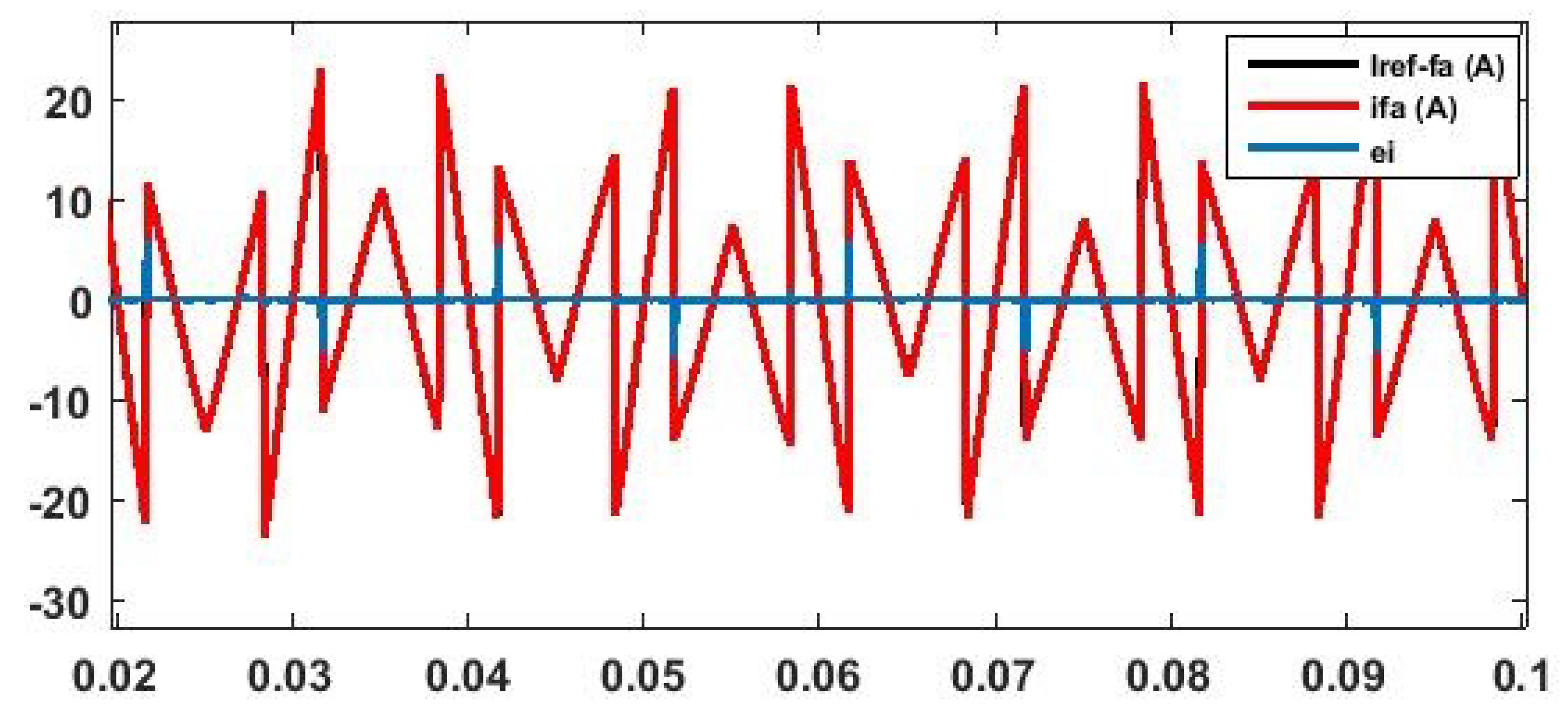
4. Simulation Results

In this section, simulation results and a discussion of some relevant theoretical issues of the proposed hybrid model as well as the control of system state variables are presented and validated using MATLAB/SIMSCAPE ELECTRICAL. Then, this will be compared to a SAPF based on a classical two-level inverter controlled by a PWM control. Starting first with the control based on PNs representation of the proposed system composed by a SAPF containing three-phase supply with 50 Hz frequency feeding a three-phase uncontrolled rectifier with an RL load.

The test is performed with a sample time equal to 10 $\mathsf{\mu }$s taking into account a delay time of 18 $\mathsf{\mu }$s in order to fix the minimum ON and OFF times of the power semiconductors. Simulation results of the global system confirm that the proposed control strategy accomplish all the control objectives. In fact, Figure 7a represents the load current of the phase a, this signal is composed by a fundamental component and harmonics, the injected current as shown in Figure 7b contains only harmonics of the identified current but in opposite phase. The injected current allows the filter to cancel all the harmonic signals and to keep only the fundamental one as presented in Figure 7c.

The following FFT analysis of the phase a of the current after filtering for our proposed system and the classical one shows the different signals composing the resulting current:

As can be seen in Figure 8 and Figure 9, the fundamental signal of 50 Hz composes 100% of the totality of signals. The THD of the proposed system is equal to 0.97%, while it is equal to 1.58% when using the conventional filter that meets the standards required by IEEE.

The measured capacitor voltages of one leg of the three-phase FCMI are balanced and they peruse the adequate references $V_{c1}=750$ V; $V_{c1}=1500$ V and $V_{c1}=2250$ V which are well defined according to the Equation (4), these results are shown in Figure 10.

Figure 11 represents the behavior of the charge and discharge ensuring the monitoring of the voltage reference of the floating capacitor $v_{c1}$. The range of the voltage variation around the reference depends on the value of the capacitance $C_1$ = $C_2$ = $C_3$ = 1 $\mathsf{\mu }$F as well as the waiting time $T=1.8\times {10}^{-7}$ s to avoid the so called “electrical over-stress”.

The error between the phase current injected by the inverter and its reference is represented by the Figure 12.

The output voltage of the first leg of the inverter is shown in Figure 13.

During a switching cycle, the number of activations and deactivations of all the switches is approximately 3200. This gives a switching 3200 × 50 Hz/2 = 80 kHz representing the switching frequency (dividing by 2 in order to allow the activation and deactivation of the switch in a single switching cycle) [36]. However, the switching frequency is equal to 16 kHz when using the conventional inverter.

Finally, the comparison between the two structures proves that the control based on a representation by Petri networks is then robust as it is able to guarantee performance criteria in stability, speed and precision for our hybrid system whose model represented varies around the theoretical or nominal model.

5. Conclusions

This paper presented a three-phase flying capacitor topology used as shunt active power filter with PNs-based control. The simulation results using MATLAB/SIMSCAPE ELECTRICAL have proved the effectiveness of this proposed study. In fact, instantaneous power theory determines with great precision the reference currents to be injected to the grid. The control based on Petri Nets representation using two cascaded representations permits the SAPF to pursue the required reference currents. Therefore, the first PNs representation determines the needed voltage level for the output current regulation, and the second one defines the switching state to ensure the required voltage level and the capacitor voltage regulation. These strategies enhance the performance and reliability of the system. Additionally, in normal operating using hysteresis control, our proposed control can mitigate harmonics of grid current with THD = 0.96% which satisfies the limits of IEEE-519 standard. Moreover, this algorithm ensures the continuity of electrical power production with good quality compared with the conventional structure. As further directions, we propose developing a fault detection algorithm for the global system.

References

1. Liu, W.; Chau, K.T.; Lee, C.H.; Jiang, C.; Han, W. A switched-capacitorless energy-encrypted transmitter for roadway-charging electric vehicles. IEEE Trans. Magn. 2018, 54, 1–6. [Google Scholar]
2. Torki, W.; Barbot, J.P.; Ghanes, M.; Sbita, L. Sparse Recovery Diagnosis Method Applied to Hybrid Dynamical System: The Case of Three-Phase DC-AC Inverter for Wind Turbine. Open Access Libr. J. 2020, 7, 1–15. [Google Scholar] [CrossRef]
3. Othman, S.; Allali, M.A.E.; Mrad, I.; Chariag, D.E.; Ghanes, M.; Sbita, L.; Barbot, J.P. Robust hybrid control based on Petri Nets for a multicellular inverter. In Proceedings of the 2020 6th IEEE International Energy Conference (ENERGYCon), Gammarth, Tunisia, 28 September–1 October 2020; pp. 143–148. [Google Scholar]
4. Krommydas, K.F.; Alexandridis, A.T. Nonlinear Analysis Methods Applied on Grid-Connected Photovoltaic (PV) Systems Driven by Power Electronic Converters. IEEE J. Emerg. Sel. Top. Power Electron. 2020, 8, 3293–3306. [Google Scholar] [CrossRef]
5. Koley, E.; Shukla, S.K.; Ghosh, S.; Mohanta, D.K. Protection scheme for power transmission lines based on SVM and ANN considering the presence of non-linear loads. IET Gener. Transm. Distrib. 2017, 11, 2333–2341. [Google Scholar] [CrossRef]
6. Khawla, E.M.; Chariag, D.E.; Sbita, L. A control strategy for a three-phase grid connected PV system under grid faults. Electronics 2019, 8, 906. [Google Scholar] [CrossRef] [Green Version]
7. Issa, W.; Sharkh, S.; Mallick, T.; Abusara, M. Improved reactive power sharing for parallel-operated inverters in islanded microgrids. J. Power Electron. 2016, 16, 1152–1162. [Google Scholar] [CrossRef] [Green Version]
8. Bhattacharya, S.; Divan, D.M.; Banerjee, B.B. Control and reduction of terminal voltage total harmonic distortion (THD) in a hybrid series active and parallel passive filter system. In Proceedings of the IEEE Power Electronics Specialist Conference (PESC’93), Seattle, WA, USA, 20–24 June 1993; pp. 779–786. [Google Scholar]
9. Karafotis, P.A.; Evangelopoulos, V.A.; Georgilakis, P.S. Evaluation of harmonic contribution to unbalance in power systems under non-stationary conditions using wavelet packet transform. Electr. Power Syst. Res. 2020, 178, 106026. [Google Scholar] [CrossRef]
10. Dehghani, M.; Mardaneh, M.; Guerrero, J.M.; Malik, O.P.; Ramirez-Mendoza, R.A.; Matas, J.; Vasquez, J.C.; Parra-Arroyo, L. A new “Doctor and Patient” optimization algorithm: An application to energy commitment problem. Appl. Sci. 2020, 10, 5791. [Google Scholar] [CrossRef]
11. Alali, M.A.E. Contribution à l’Etude des Compensateurs Actifs des Réseaux Electriques Basse Tension (Automatisation des systèMes de Puissance éLectriques). Ph.D. Thesis, University of Strasbourg, Strasbourg, France, 2002. [Google Scholar]
12. Wang, X.; Blaabjerg, F. Harmonic stability in power electronic-based power systems: Concept, modeling, and analysis. IEEE Trans. Smart Grid 2018, 10, 2858–2870. [Google Scholar] [CrossRef] [Green Version]
13. Alali, M.A.; Shtessel, Y.B.; Barbot, J.P. Grid-Connected Shunt Active LCL Control via Continuous SMC and HOSMC Techniques. In Variable-Structure Systems and Sliding-Mode Control; Springer: Cham, Switzerland, 2020; pp. 275–308. [Google Scholar]
14. Mrad, I. Observabilité et Inversion à Gauche des systèmes Dynamiques Hybrides. Ph.D. Thesis, École Nationale D’ingéNieurs de Gabès, Cergy-Pontoise, France, 2019. [Google Scholar]
15. Barbot, J.P.; Saadaoui, H.; Djemai, M.; Manamanni, N. Nonlinear observer for autonomous switching systems with jumps. Nonlinear Anal. Hybrid Syst. 2007, 1, 537–547. [Google Scholar] [CrossRef]
16. Meynard, T.; Foch, H. Electronic Device for Electrical Energy Conversion between a Voltage Source and a Current Source by Means of Controllable Switching Cells. U.S. Patent 5,737,201, 7 April 1998. [Google Scholar]
17. Depenbrock, M. Direct self-control (DSC) of inverter fed induktion machine. In Proceedings of the 1987 IEEE Power Electronics Specialists Conference, Blacksburg, VA, USA, 21–26 June 1987; pp. 632–641. [Google Scholar]
18. Zouari, M.; Baklouti, N.; Sanchez-Medina, J.; Kammoun, H.M.; Ayed, M.B.; Alimi, A.M. PSO-Based Adaptive Hierarchical Interval Type-2 Fuzzy Knowledge Representation System (PSO-AHIT2FKRS) for Travel Route Guidance. IEEE Trans. Intell. Transp. Syst. 2020. [Google Scholar] [CrossRef]
19. Jin, Z.; Meng, L.; Guerrero, J.M.; Han, R. Hierarchical control design for a shipboard power system with DC distribution and energy storage aboard future more-electric ships. IEEE Trans. Ind. Inform. 2017, 14, 703–714. [Google Scholar] [CrossRef] [Green Version]
20. Gateau, G. Contribution à la Commande des Convertisseurs Statiques Multicellulaires Série: Commande non linéaire et Commande Floue. Ph.D. Thesis, Institut National Polytechnique de Toulouse, Toulouse, France, 1997. [Google Scholar]
21. Delmas, L.; Gateau, G.; Meynard, T.A.; Foch, H. Stacked multicell converter (SMC): Control and natural balancing. In Proceedings of the 2002 IEEE 33rd Annual IEEE Power Electronics Specialists Conference, Cairns, Australia, 23–27 June 2002; Volume 2, pp. 689–694. [Google Scholar]
22. Tachon, O. Commande Découplante Linéaire des Convertisseurs Multicellulaires Série: Modélisation, Synthèse et Expérimentation. Ph.D. Thesis, Institut National Polytechnique de Toulouse, Toulouse, France, 1998. [Google Scholar]
23. Xiong, R.; Cao, J.; Yu, Q.; He, H.; Sun, F. Critical review on the battery state of charge estimation methods for electric vehicles. IEEE Access 2017, 6, 1832–1843. [Google Scholar] [CrossRef]
24. Alali, M.; Saadate, S.; Chapuis, Y.; Braun, F. Energetic study of a series active conditioner compensating voltage dips, unbalanced voltage and voltage harmonics. In Proceedings of the 7th IEEE International Power Electronics Congress, Technical Proceedings, CIEP 2000 (Cat. No.00TH8529), Acapulco, Mexico, 15–19 October 2000. [Google Scholar]
25. Djondiné, P.; Barbot, J.P.; Ghanes, M. Comparison of Sliding Mode and Petri Nets Control for Multicellular Chopper. Int. J. Nonlinear Sci. 2018, 25, 67–75. [Google Scholar]
26. Amghar, B.; Darcherif, A.; Barbot, J.P. Z(TN)-Observability and control of parallel multicell chopper using Petri nets. IET Power Electron. 2013, 6, 710–720. [Google Scholar] [CrossRef]
27. Barbot, J.P.; Levant, A.; Livne, M.; Lunz, D. Discrete differentiators based on sliding modes. Automatica 2020, 112, 108633. [Google Scholar] [CrossRef]
28. Salinas, F.; Ghanes, M.; Barbot, J.P.; Escalante, M.F.; Amghar, B. Modeling and control design based on petri nets for serial multicellular choppers. IEEE Trans. Control. Syst. Technol. 2014, 23, 91–100. [Google Scholar] [CrossRef]
29. Vázquez, M.A.G.; Salinas, F.S.; Gutiérrez, M.F.E. Capacitor and Input Voltage Estimation Scheme for Flying Capacitor Multilevel Converters Modelled as a Petri Net. ISA Transactions; Elsevier: Amsterdam, The Netherlands, 2021. [Google Scholar]
30. Petri, C.A. Kommunikation Mit Automaten; Mathematisches Institut der Universität Bonn: Bonn, Germany, 1962. [Google Scholar]
31. Reveliotis, S.A. Real-Time Management of Resource Allocation Systems: A Discrete Event Systems Approach; Springer Science & Business Media: Berlin, Germany, 2006; Volume 79. [Google Scholar]
32. Silva, M. On the history of discrete event systems. Annu. Rev. Control 2018, 45, 213–222. [Google Scholar] [CrossRef]
33. Farhat, M.; Barambones, O.; Sbita, L. A new maximum power point method based on a sliding mode approach for solar energy harvesting. Appl. Energy 2017, 185, 1185–1198. [Google Scholar] [CrossRef]
34. Alali, M.A.; Barbot, J.P. A Lyapunov approach based higher order sliding mode controller for grid connected shunt active compensators with a LCL filter. In Proceedings of the 2017 19th European Conference on Power Electronics and Applications (EPE’17 ECCE Europe), Warsaw, Poland, 11–14 September 2017. [Google Scholar]
35. Akagi, H.; Kanazawa, Y.; Nabae, A. Instantaneous reactive power compensators comprising switching devices without energy storage components. IEEE Trans. Ind. Appl. 1984, IA-20, 625–630. [Google Scholar] [CrossRef]
36. Sadigh, A.K.; Dargahi, V.; Corzine, K.A. New active capacitor voltage balancing method for flying capacitor multicell converter based on logic-form-equations. IEEE Trans. Ind. Electron. 2016, 64, 3467–3478. [Google Scholar] [CrossRef]
Figure 1. General structure of a shunt active power filter.
Energies 14 05335 g001
Figure 2. Power topology of the proposed SAPF.
Energies 14 05335 g002
Figure 3. Proposed control scheme based on Petri Nets representation.
Energies 14 05335 g003
Figure 5. Behavior of the voltage level corresponding to the output filter current following the operation region.
Energies 14 05335 g005
Figure 6. Petri Nets representation for capacitor voltages regulation.
Energies 14 05335 g006
Figure 7. Currents of the proposed SAPF: (a) Load current of the phase a before filtering. (b) Injected current. (c) Supply current of the phase a after filtering.
Energies 14 05335 g007
Figure 8. FFT analysis of the phase a current after filtering using FCMI filter.
Energies 14 05335 g008
Figure 9. FFT analysis of the phase a current after filtering using conventional filter.
Energies 14 05335 g009
Figure 10. Floating capacitor voltages and their corresponding references of one leg of a three-phase FCMI.
Energies 14 05335 g010
Figure 11. Behavior of the charging and discharging of capacitor C 1 .
Energies 14 05335 g011
Figure 12. Error between the injected current and its reference.
Energies 14 05335 g012
Figure 13. FCMI phase to phase voltage.
Energies 14 05335 g013