Abstract
Thunderstorm downbursts have been reported to cause damage or failure to wind turbine arrays. We extend a large-eddy simulation model used in previous work to generate downburst-related inflow fields with a view toward defining correlated wind fields that all turbines in an array would experience together during a downburst. We are also interested in establishing what role contrasting atmospheric stability conditions can play on the structural demands on the turbines. This interest is because the evening transition period, when thunderstorms are most common, is also when there is generally acknowledged time-varying stability in the atmospheric boundary layer. Our results reveal that the structure of a downburst’s ring vortices and dissipation of its outflow play important roles in the separate inflow fields for turbines located at different parts of the array; these effects vary with stability. Interacting with the ambient winds, the outflow of a downburst is found to have greater impacts in an “average” sense on structural loads for turbines farther from the touchdown center in the stable cases. Worst-case analyses show that the largest extreme loads, although somewhat dependent on the specific structural load variable considered, depend on the location of the turbine and on the prevailing atmospheric stability. The results of our calculations show the highest simulated foreaft tower bending moment to be 85.4 MN-m, which occurs at a unit sited in the array farther from touchdown center of the downburst initiated in a stable boundary layer.
1. Introduction
Thunderstorm downbursts produce strong downdrafts and low-level diverging outflow that can generate potentially damaging surface winds [1]. This phenomenon has been studied for decades within the meteorological community, focusing mostly on the formation and dynamics of downbursts along with the associated risks in aviation. From an engineering point of view, straight-line gusts near the surface pose great risks of potential damage/destruction to buildings and structures [2,3,4], as well as to turbines in a wind farm [5]. Accordingly, this study seeks to evaluate the effects of downburst winds on a representative wind farm by examining the response of individual turbines as they experience high wind velocities and rapid wind direction changes during such simulated events.
The characteristics of velocity fields during a thunderstorm downburst have been shown to be highly dependent on the prevailing atmospheric stability of the ambient environment [6]. Downbursts frequently occur in the late afternoon, during the so-called evening transition (ET) period when the atmospheric boundary layer (ABL) changes from convective to stable. The convective boundary layer (CBL) is characterized by higher variability in wind velocities due to large turbulent eddies generated from the daytime surface heating. After sunset, the eddies are greatly reduced because the cooling surface causes formation of stably stratified conditions where the nocturnal stable boundary layer (SBL) develops [7]. Therefore, it is of interest to study stability-related influences on downburst winds and their distinct effects on loads on individual turbines in arrays. To carry out such a study, traditional analytical approaches [8,9,10] used to describe downburst wind fields are inadequate, as they do not reflect the underlying physics and realistic dynamics of ABL turbulent fields. By contrast, in recent years, large-eddy simulation (LES) is increasingly used to model downburst winds [11,12,13,14,15]. Moreover, by using an initiating cooling source aloft [11,12,16], it is possible to perform idealized simulations with downbursts immersed into turbulent fields of different stabilities. The approach, originally proposed by Anderson et al. [17], does not require the full storm to be resolved; therefore, both the domain size and computational expense can be reduced considerably using an LES model. Such LES-generated wind fields, which can reproduce the principal characteristics of downbursts and produce high-fidelity data sets comparable to observations, are considered appropriate inflow fields for turbine loads assessment and for the estimation of risks to wind farms during downbursts.
Over several years, several research studies have been undertaken that involved analytically studying downburst models for structural engineering applications. Such applications include downburst wind loading on transmission lines and towers [18,19,20], slender structures including vertical masts [21,22,23], and tall buildings [24,25,26]. On the other hand, to consider the complex flow features of downbursts and not only basing them on idealized mathematical models, other studies have been conducted that have involved the simulation of downburst-related loading on structures informed by wind tunnel tests on buildings and structures [27,28,29,30,31,32], including the consideration of a wind turbine in such simulated fields [33]. In recent years, other studies have placed an emphasis on the estimation of downburst-induced loads by employing numerical models for transmission lines [34,35], buildings [36,37], and bridges [38]. Generally speaking, numerical simulation, especially using LES with consideration of ABL turbulent fields, represents a most appropriate approach for describing the complex behavior of downbursts and for realistically capturing the associated turbulence characteristics. However, applications of LES in the investigation of downburst-induced loads on individual wind turbines or turbine arrays are limited in the literature.
In the present study, we extend the work of Lu et al. [39] to allow the estimation of loads on turbines in an array; we used LES-simulated downburst events and associated wind fields during various stability regimes. By evaluating loads on the different turbines over an entire array, one can more systematically assess the influence of contrasting ambient stability conditions at different locations relative to the touchdown center of the downburst as it develops and dissipates. Atmospheric stability has significant influence on the evolution of downbursts to a mature stage; this results in load differences for turbines situated close to and far from touchdown. The geostrophic wind direction also changes with stability and affects the development track of the initiated downbursts. Thus, it is of great interest to study loads on the spatially distributed units in a turbine array rather than only those on a single isolated turbine. The wind farm/array configuration with multiple turbine units, proposed by Nguyen and Manuel [40], is used in our illustrations, along with a framework for turbine inflow generation similar to that used by Park et al. [41] and by Lu et al. [42]. The methodology describing how downburst-related wind fields are generated and how loads are estimated on turbine units in a wind farm is demonstrated in Section 2. In Section 3, we summarize key features in the structure of the downburst velocity field over the spatial coverage of the wind farm. Next, in Section 4, selected turbine load variables are examined and related to the associated inflow fields and to downburst-and-stability-related physical characteristics. In Section 5, the effects of contrasting atmospheric stability regimes are assessed in statistical analyses of both the LES-generated wind fields and the associated simulated loads. Finally, in Section 6, cases that result in the most extreme loading scenarios on units in the selected turbine array during the downburst events are studied and some concluding remarks are presented.
2. Methodology
In this section, the LES model used to generate downburst events is briefly summarized. We also describe how the selected turbine array is arranged within the computational domain for the simulations and how inflow fields are generated for each turbine unit. The aeroelastic simulation model used to calculate turbine loads is also introduced and details related to its use in this study are presented.
2.1. Downburst Model Using Large-Eddy Simulation
In order to generate downburst wind fields in the ABL under different atmospheric stability conditions, a pseudo-spectral LES model [43] is applied, together with a cooling source approach [11,12,17] that mimics the evaporative cooling system. We extend the model and framework of our previous studies [6,39,42] in order to allow the risk assessment of multiple turbines in a wind farm arranged spatially in a rectilinear array. The computational domain for the full-field simulation is set at 10 km × 10 km × 3 km, with a grid resolution of 27.78 m in each direction. Figure 1 outlines the simulation procedure employed for generating the full-domain wind fields. We initialize the model with a constant temperature of 300 K and a temperature inversion (of 6 K km) at the initial boundary layer height of 1.5 km. The wind field is initialized with a constant profile of 8 m s in the x-direction. In order to represent average land cover conditions over North America, an aerodynamic roughness length of 0.1 m is assumed. For the first two hours of spin up, the surface temperature is set at 303 K to drive convection (this represents Phase I). Next, in Phase II, the surface temperature is decreased at a constant rate (with time) so as to generate intermediate ABLs with five different atmospheric stabilities including convective (C1), weakly convective (C2), near-neutral (N), weakly stable (S1), and stable (S2) conditions. At five different times, separated by one hour, the full wind field is saved in order to create initial conditions for downbursts in contrasting atmospheric stabilities. In Phase III, the cooling source approach proposed by Anderson et al. [17] and employed by Orf et al. [44] and Anabor et al. [11] is used with the time span for the cooling rate intensity function set at 6 min. This relatively short time span is selected to limit the possibility of secondary surges during the downburst; the outflow is allowed to propagate over the entire domain within the simulation time of 15 min. Since periodic boundary conditions are used in the LES runs, we are permitted to shift the cooling source location by 5 km in both the x and y directions and, thus, derive four different fields (referred to as 0x0y, 0x5y, 5x0y, and 5x5y to reflect the cooling source location), as shown in Figure 2. These four fields are shown in an earlier study [6] to have similar levels of ambient turbulence intensity for cases of individual stability; in other words, the choice of cooling source location has limited effect on the turbulence characteristics of generated downbursts. Each of the four fields is used separately as initial fields in which downburst events are generated to yield a suite of cases with distinctly sampled turbulence that then offer a robust ensemble for each stability case. Thus, in total, LES runs are carried out in this study. Additional details related to the downburst simulations can be found in the studies by Hawbecker et al. [6] and Lu et al. [39].
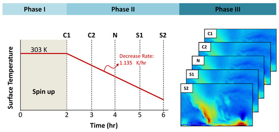
Figure 1.
Three phases in the procedure for generating downburst wind fields during period of contrasting atmospheric stability (Lu et al. [39]).
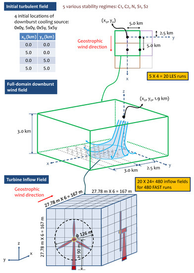
Figure 2.
Framework for inflow generation for multiple turbine units in an array during LES-simulated downbursts carried out within different stability regimes.
2.2. Wind Farm Model
Figure 3 shows a schematic diagram depicting a turbine array in the computational domain of the LES model. Note here that the turbine models are completely offline in these computations and do not have any interaction with the simulated downburst wind field; only the flow fields at the specified locations of the turbines are extracted to define the inflow fields for each turbine’s load calculations. As observed in the figure, the example of case 0x0y is presented with the cooling source located at , , and km in a global coordinate system. We extend the framework defined by Nguyen et al. [40] to establish a array of turbine units placed symmetrically with respect to the x axis (i.e., the lateral symmetry implies that lies along the center line of the array). The four rows with six turbines arranged laterally in each row have their vertical y–z rotor planes displaced from the cooling source by 2.5, 3.5, 4.5, and 5.5 km, respectively, in the longitudinal (x) direction. The 24 turbine units in total are denoted by index numbers as shown, and they are all separated from each other by 1 km in both x and y directions. This separation is roughly equal to eight rotor diameters, , where D is 126 m for the selected 5 MW turbines considered part of the wind farm. For convenience in the following discussions, we split the turbines into six groups according to their location in the array; these groups are as follows: southwest (SW), southeast (SE), middle-west (MW), middle-east (ME), northwest (NW), and northeast (NE). The cooling source center for the downburst is initiated at = (0.0 km, 0.0 km, 1.9 km) for the selected case (0x0y). Considering the westerly geostrophic wind, the downburst is expected to translate from the west all the way through the wind farm, as depicted in the 3-D diagram presented in Figure 2.
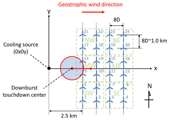
Figure 3.
A schematic diagram showing turbine units in a rectilinear array and a possible downburst touchdown location in the LES computational domain. Case 0x0y is illustrated where the cooling source is initiated at = (0.0 km, 0.0 km, 1.9 km).
2.3. Turbine-Scale Inflow Generation
The turbine-scale inflow fields, corresponding to the 24 spatially separated turbine units, are extracted from the LES wind fields of the downburst events. Figure 2 shows the framework for load assessment of all turbines in the array using these LES-based inflow fields. We employ a similar procedure to that used in other earlier studies [41,42] in order to generate the inflow fields for the turbine units of the array. In order to account for appropriate aerodynamic forces on the turbine blades in a 3-D space when nacelle yaws and associated control actions are included, a 167 m × 167 m × 167 m 3-D inflow velocity field for each turbine is used instead of a 2-D planar velocity field; such a representation is especially needed during significant wind direction changes during a downburst. Here, we note that dynamic wake losses are not accounted for in our simulations; in strong wind conditions, such losses are insignificant compared to the dominant transient wind velocity fields such as those experienced in downbursts. Other studies have shown that wake effects included, for example, using an unsteady vortex lattice method (UVLM) that can represent turbine wakes, but these are of importance only in low wind speed regimes [45]. Wake effects are of lesser concern than the structural safety of turbine blades and towers during a downburst. Such an approach to describe the inflow fields on array units was also utilized in a similar study by Nguyen et al. [40], except that LES was not employed in that study. The inflow box with a 27.78 m grid spacing on each side is centered at each turbine hub with grid points. Vertical levels over 14 m 181 m for each box allow spatial coverage over the entire rotor. With a total simulation time of 15 min and a time step of 0.1 s, the 4-D (describing three orthogonal velocity components in a 3-D space and at discrete time intervals) inflow fields with 9000 frames for each turbine are generated. For 24 turbines in the array, combined with the 20 LES runs (four different cooling source locations and five different atmospheric stabilities considered), we have inflow fields in total for the turbine load simulations. As observed in Table 1 (same as in Lu et al. [39]), run No. 9 represents a “control” run that is alone used to first investigate the characteristics of the downburst-related wind field over the entire array. Later, statistical analyses are performed by using all the inflow fields in order to draw comparisons among the various downburst cases simulated.

Table 1.
List of all LES runs indicating atmospheric stability condition and cooling source location.
2.4. Turbine Load Simulations
The NREL 5-MW onshore baseline wind turbine model [46] is used with the open-source program, FAST (Fatigue, Aerodynamics, Structures, and Turbulence) Version 8 [47], for the turbine loads calculations using the LES-generated inflow fields as input. The properties and dimensions of the turbine model are presented in Table 2 together with a schematic diagram in Figure 4 showing the three turbine load variables of interest: OoPBM (the blade root out-of-plane bending moment), FATBM (the fore-aft tower bending moment) and TTYM (tower-top yaw moment). The rotational direction seen from the reference frame defined in FAST is clockwise when looking downwind. The pitch control action is activated in the model when the hub-height inflow wind speed exceeds the rated wind speed of 11.4 m s. An increased pitch angle for the turbine blades mitigates loads. Yaw control is also assumed for the turbine model to limit yaw error or misalignment; however, the nacelle yaw can match the inflow wind direction only if the rate of change of wind direction is low. The maximum nacelle yaw rate is limited to 0.3° per s; the yaw rate is set equal to the wind direction change rate if the latter does not exceed the maximum nacelle yaw rate. The UserWind module is employed with FAST to read wind data files generated by the LES model. The time step for the load simulation is set to 0.0125 s throughout the 15 min duration of each downburst event. In order to assure numerical stability of the FAST runs over the wide range of simulated wind speeds, the steady-state BEM (blade element momentum) model is used to calculate turbine loads. We note here that the prediction of dynamic loads is less accurate with the BEM model compared to other choices such as the generalized dynamic wake (GDW) model [48]; however, our primary aim is to compare turbine loads during downbursts and our focus is on differences in atmospheric stability to be accounted for. In subsequent statistical analyses of turbine loads, the 10-min extreme load (ExL) for each of the three load types is extracted from the entire 15 min time series for all the 480 FAST runs. The first 300 s of data are discarded to eliminate transient effects in the FAST simulations.
Table 2.
Properties and dimensions of the selected 5-MW NREL turbine model.
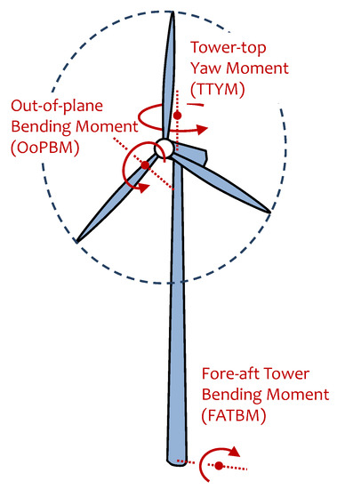
Figure 4.
Schematic diagram of the turbine model showing the three types of loads, OoPBM, FATBM, and TTYM, used in this study.
3. Characteristics of Downbursts Interacting with Wind Turbine Array
In a previous study, Hawbecker et al. [6] discussed characteristics of downburst wind fields in different stability regimes. In another study [39], wind velocities at turbine scale during downbursts were studied. Here, we highlight characteristics of downburst-related wind velocities and wind direction changes that influence turbine loads over an entire wind farm.
3.1. Spatial Characteristics of the Downburst Wind Field
Figure 5 shows the velocity field on a laterally centered x-z plane ( km) of the simulation domain at s for the selected case N-0x0y (N indicates neutral). Only the longitudinal and vertical velocity components (U and W) are considered. Downdrafts initiated from the cooling source at = (0.0 km, 1.9 km) can be clearly seen in the figure. The downdraft results in the propagation of outflows and the formation of a ring vortex. The largest horizontal wind speed frequently occurs below the ring vortex and can pose great risks of turbine damage. From an earlier study [39], we have seen that the height of the center of the ring vortex influences surface extreme winds. As can be observed in the figure, the height of the vortex center is at about 350 m AGL (above ground level) in the neutral case. The study by Hawbecker et al. [6] showed that this ring vortex height can increase as stability increases.
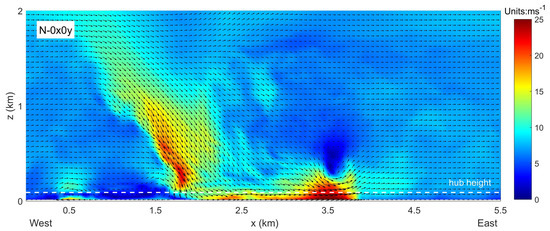
Figure 5.
Filled contours of wind velocities on a laterally centered vertical cross-section ( km) for the case N-0x0y at s. The color map denotes the magnitude of the resultant wind velocity, .
It is of interest to note how extreme winds diverge and dissipate with the development of a downburst throughout the spatially distributed turbines in an array. Figure 6 shows filled contours of hub-height horizontal wind velocities for the cases, C1-0x0y, N-0x0y, and S2-0x0y. Three snapshots of the wind fields are presented for each case at simulation times of 465,570 and 675 s. Only the hub-height horizontal velocity components ( and ) are considered, with the color map denoting the magnitude of . The contours clearly show how the downburst strikes the wind farm from a mature stage to a dissipating stage. At 465 s, the ring vortex is well-developed and a distinct band of wind speeds greater than 20 m s at hub height can be observed. The ring vortices for the N and S2 cases have already struck the second row of turbines (i.e., Nos. 2, 6, 10, 14, 18, and 22), but the extreme winds in the C1 stability case have not yet reached that row due to the greater interaction with the ambient turbulence, which impedes the downburst’s forward propagation. Due to Coriolis forcing, the ambient wind direction deviates to the northeast as the stability increases. This also affects the trajectory of the downburst and changes the impacted area of the array. At 570 s, the ring vortex in the C1 case has started to dissipate. Outflows near the southeast section have already become disorganized. This is probably due, again, to deviation of the ambient wind direction. Even if there is only a slight wind direction deviation in the convective case (∼3.2° on average), it still introduces asymmetry in the downburst field/propagation and weakens the southeast outflows. The ring vortices in the N and S2 cases last longer; the neutral (N) case appears to have started dissipating by s. At that time, however, outflows in the S2 case are still observed to be well-organized as they pass over the northeast corner of the array, whereas the outflows in the convective case are almost completely dissipated due to the ambient turbulence. Based on these features of the downburst propagation in the different stability regimes, it is interesting to examine the wind fields and associated turbine loads for the six turbine groups at different locations within the turbine array.
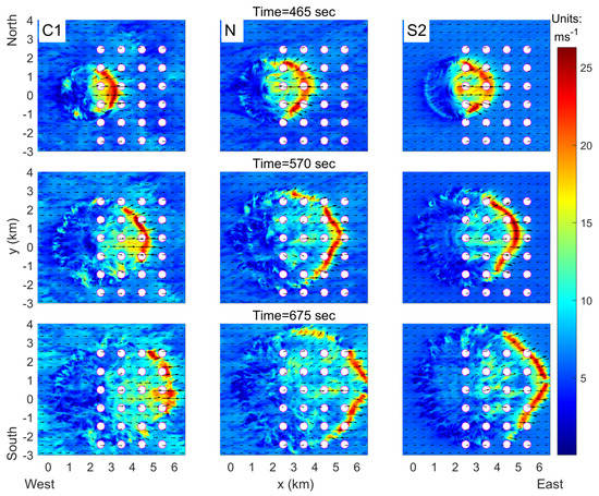
Figure 6.
Filled contours of the horizontal velocity at hub height for cases C1-0x0y, N-0x0y, and S2-0x0y at t = 465, 570 and 675 s. The color map denotes horizontal wind speed. Specific locations of turbines are denoted by white circles.
3.2. Characteristics of Turbine-Scale Wind Fields
In a previous study [39], we analyzed wind velocities at turbine scale along the center line of the downburst propagation path. This investigation is extended to examine the wind field over the entire turbine array. In Figure 7, the time series of the hub-height horizontal wind speed (), vertical wind speed (), and horizontal wind direction () are shown for the case N-0x0y. Six flow fields are selected: four from the corners and two near the center line of the array. From the time series of the horizontal wind speed, large wind surges with high extreme wind speeds can be observed for the center line turbines, X9 and X12. The maximum wind speeds at the four corners are relatively lower because the direct impact is greater along the direction of the downburst propagation. Since the ambient winds tend to deviate the flow field toward the northeast corner, the maximum horizontal wind speeds at the top (north) two units, X21 and X24, are greater than those at the bottom (south) two units, X1 and X4; moreover, the extreme wind speed at X24 is greater than that at X21. As observed from the vertical velocity variation, an updraft followed by a rapid downdraft is observed when the ring vortex passes each turbine; it is at this same time that the extreme horizontal wind speed also occurs. The maximum vertical wind speed is larger as one becomes closer to the downburst propagation line. The vertical velocities are not observed to be sensitive to the change in ambient wind direction. For the change in wind direction at hub height, it is found that the variability increases after the maximum outflow has occurred. The variability also becomes larger when the flow field is closer to the downburst propagation line. Depending on which side (laterally) the flow field of interest is located, the wind direction variation can have either a positive or a negative first peak. The larger first peak magnitude occurs at units X1 and X21, for which the outflow direction deviates the most from the direction of the ambient winds. For units almost aligned with the downburst propagation direction (i.e., X9 and X12), the primary surge of the downburst does not change the wind direction very much. However, the wind field at X9 continues to be disturbed by the sustained cool downdrafts after the outflows spread. Turbulence caused by the downburst can introduce additional variability and greater deviation in the wind direction. In all our simulations, none of the turbines experience a fully reversed (upwind) outflow of the same magnitude as the first forward outflow as had been reported in other downburst studies [10,49]; thus, there is no reversed wind peak in any of the horizontal wind speed time series.
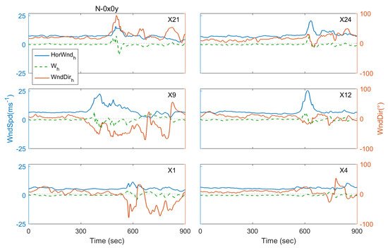
Figure 7.
Time series of hub-height horizontal and vertical wind speed and horizontal wind direction for selected turbines in the control case N-0x0y.
Figure 8 shows location-specific wind roses based on time series of the horizontal velocity at hub height at the same six selected unit locations, for case N-0x0y, that were considered in Figure 7. The frequency of winds is plotted by wind direction with color bands showing the range of horizontal wind speed; the radial extent of each wind direction bin is proportional to the frequency of that bin. The longest spoke (or radial sector) in each plot generally describes the dominant or mean direction of ambient winds, with wind speed less than 9 m s. It is found that the ambient winds are directed largely from west to east at all units with deviation caused by Coriolis forces. When the outflow passes each unit, it results in shorter wind rose spokes with higher wind speeds that deviate from the ambient wind direction. Depending on the specific locations of the units, this pattern varies; for instance, wind roses in the top row (X21–X24) show a few short spokes deviating to the south while those in the bottom row (X1–X4) show flow deviations to the north. The X9 unit close to the downburst’s touchdown center suffers the strongest outflows with large variation in wind direction and experiences high winds for the longest time. Thus, this unit’s wind rose clearly shows the most high-speed contribution. Compared to an earlier study on downburst winds using stochastic wind field models [50], the LES-generated wind velocities show larger variability of outflow velocities. When considering simplified wind fields modeled by analytical equations in that study [50], along with superimposed turbulent fields, the wind velocities generally vary along the defined analytical curves with residual turbulence reaching up to about 10 m s at most, which is very different from the wind field time series observed in Figure 7. The LES-simulated wind velocities have greater variability than the predicted analytical (non-turbulent) curves, and the turbulent fluctuations are also seen at lower frequencies than those simulated by stochastic models [50]. The relationships between fluctuating (turbulent) and non-fluctuating components of the wind field are shown to be much more complex in the LES-generated data; this can result in increased uncertainty in associated turbine loads on individual units in a turbine array.
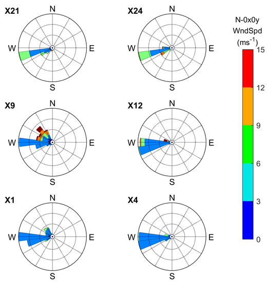
Figure 8.
Wind roses of the horizontal velocity at hub height for selected turbine-scale wind fields in the control case N-0x0y.
4. Case Studies of Wind Turbine Loads
In the preceding section, an understanding of how the velocity fields vary over the wind farm has been established. We next relate wind velocity to the actions of the turbine control system, as well as to turbine loads. Then, the performance of turbines throughout the wind farm can be discussed.
4.1. Relationship among Velocity Field, Turbine Loads, and Turbine Control System
In an earlier study [39], a series of investigations was performed with a view toward establishing relationships between the velocity fields and turbine loads at a single turbine. In the present study, we only very briefly revisit the findings using the simulated 3-D turbine-scale inflow fields and associated turbine loads. Figure 9 shows the time series of hub-height horizontal wind speed (), hub-height vertical wind speed (), pitch angle (PitAng), hub-height wind direction (), nacelle yaw angle (YawAng), yaw error (YawErr), and turbine loads (OoPBM, FATBM, and TTYM) for a selected single unit X10 in the control case N-0x0y. The selected turbine is located at the center of the wind farm so that the primary surge of the outflow is clearly observed in the horizontal wind curve with relatively small changes in wind direction (°). When the horizontal wind speed is greater than the rated wind speed of 11.4 m s, the pitch control action is triggered, which results in an increase in the pitch angle of the turbine blades (red curve) and directly relieves the streamwise wind pressure. The time series of the OoPBM and FATBM loads closely follow the curves for and PitAng; thus, there are two evident load peaks at the start and end times of the period of activated pitch control. Generally, the extreme load (shown by a red star marker) for OoPBM and FATBM occurs at the start of this period (a second peak is also observed at the end of this period). By contrast, TTYM loads show a more complex pattern; since the yaw moment is sensitive to the asymmetric loading applied on the three blades, forces in both the horizontal and vertical directions can influence these TTYM loads. We have found that there is a higher probability that the extreme TTYM load occurs when vertical winds convert from updrafts to downdrafts (see the green dashed curve). A noticeable up-and-down pattern is observed in the TTYM curve when the direction of changes suddenly and an extreme load then is evident. Yaw error, resulting from a slow and heavy (inertia-driven) nacelle unable to keep up with a rapid rate of change in wind direction, is also considered a factor that affects the yaw moment. Since the maximum change rate for the nacelle yaw angle (blue dashed curve) is limited to 0.3° per s, fluctuations in the yaw error (magenta curve) are clearly observed to increase when the change in wind direction (yellow curve) increases after the primary surge of the downburst. This in turn can result in large fluctuations in the TTYM load.
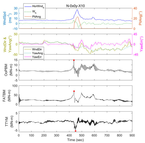
Figure 9.
Time series of hub-height horizontal wind speed (), hub-height vertical wind speed (), pitch angle (PitAng), hub-height wind direction (), nacelle yaw angle (YawAng), yaw error (YawErr), and turbine loads (OoPBM, FATBM, and TTYM) for a selected single unit (X10) in the control case N-0x0y.
4.2. Characteristics of Load Time Series
Based on an understanding of the relationship between the inflow wind field and turbine loads, as well as of the influence of turbine control actions, we further investigate characteristics of load time series throughout the turbine array. Figure 10 and Figure 11 show the time series of TTYM and OoPBM, respectively, for the same six turbine units selected in case N-0x0y that were considered before. The time series data are trimmed to 300–900 s since information prior to the downburst is not of significant interest in the subsequent discussion. Time series of , , PitAng, and YawErr are presented in order to facilitate direct comparisons. The time series for FATBM show a similar trend to that for OoPBM and are, therefore, not shown here.
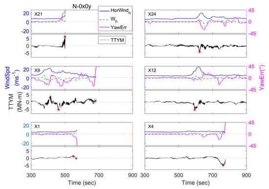
Figure 10.
Time series of hub-height horizontal and vertical wind speed as well as yaw error and TTYM load for six selected turbine units in the control case N-0x0y. The extreme load in each case is denoted by a red star marker.
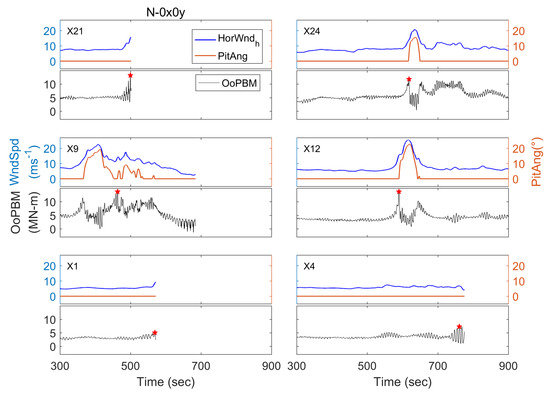
Figure 11.
Time series of hub-height horizontal wind speed, pitch angle, and OoPBM load for six selected turbine units in the control case N-0x0y. The extreme load in each case is denoted by a red star marker.
In Figure 10, we noticed that the FAST simulations for the turbine units at the array corners (i.e., X1, X4, and X21) cannot be completely run through the entire 900 s simulation time because FAST is forced to stop when the yaw error exceeds 45° in the simulations. A limitation of the BEM model used is that the dynamic load calculations are inaccurate with such a large yaw error; hence, simulated loads beyond the forced stop point are excluded. In our wind farm model, the turbine units most laterally offsetted, on both sides of the downburst trajectory, tend to experience the most rapid changes in wind direction. When the yaw control system cannot keep up with this rapid direction change, the maximum permissible yaw error limit is reached. The turbine unit, X24, does not experience a large yaw error probably because the deviated direction of the ambient winds has already adjusted the nacelle yaw to a better orientation; thus, there is no premature termination of the FAST run for that case. The turbine unit, X9, is located along the downburst center line. The yaw error is, therefore, not large as the outflow passes this unit. However, sustained downdrafts after the downburst surge results in turbulence in the dominant wind direction and increases the yaw error even at relatively low wind speeds. Thus, we observe that the simulation for X9 has stopped a short while after the maximum outflow occurs. The occurrence time for TTYM extremes is less clear and, thus, rather uncertain. For the X9 unit in the laterally centered row, the extreme TTYM load is closely related to lasting intense winds that follow the maximum outflow. The units, X4 and X21, at the edges, are observed to experience extreme TTYM loads right at the time of the rising downburst surge. The simulations are, however, terminated at about the time of occurrence of these extreme loads. The cases of units X1, X12, and X24 (also at the edges) show greater uncertainty in the extreme loads as they occur at a time that appears to not be exactly related to the outflow. This could be attributed to the sensitivity of TTYM loads relative to the asymmetric loading on the turbine blades. Transient turbulence and wind shear could also help to explain these extreme yaw moments.
As can be observed from Figure 11, the extreme OoPBM load is relatively more predictable (than TTYM) based on the time series of horizontal wind speed and pitch angle. For the units, X1, X4, and X21, the extreme load occurs at a time close to when the FAST run is terminated, since the largest wind speed appears at a time when the rising trend in the load is interrupted. The extreme loads at unit X12 and X24 occurs at the start time of the triggered pitch control action. The unit X9 experiences a direct impact of the primary surge of the downburst; however, there is also a secondary surge observed and the extreme load at this unit occurs at the start time of the second pitch control activation.
5. Effects of Atmospheric Stability
Based on the downburst wind field simulations and the impact on the selected wind farm, the effect of atmospheric stability can now be studied through statistics calculated from the 480 flow fields and associated load simulations.
5.1. Statistics of Wind Fields
In order to compare characteristics of the downburst wind fields for the various stability regimes, we consider statistics according to the same six turbine groups considered earlier. Figure 12 presents the statistics of the maximum horizontal wind speed at hub height for the five atmospheric stabilities in the six turbine groups. All of the data from the 480 turbine-scale flow fields are used to create the box plots shown. First, we note that, in general, the extreme wind speeds are somewhat larger in the east groups for each stability case. This can be explained by the fact that the outflow requires some time and space to organize after the descent of the downburst; thus, the extreme wind speeds become higher at downwind locations farther from the touchdown center.
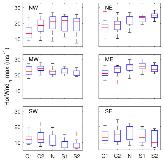
Figure 12.
Box plots of the maximum horizontal wind speed at hub height for different atmospheric stabilities using statistics from the 480 flow fields. The six turbine groups are separated into different subplots. Each box represents samples (representing all combinations of the 4 units per turbine group with 4 initial locations of the cooling source).
We next compare extreme winds across all five stability cases. The trend in the middle-west (MW) turbine group shows that the convective cases experience larger extreme wind speeds than the stable cases. This result is consistent with our previous conclusion that the ring vortices in the convective cases develop faster and result in stronger outflows near the touchdown center. As the propagation of the downburst continues, however, these ring vortices in the convective cases start to dissipate and decrease the extreme wind speeds as observed in the middle-east (ME) panel. Notice that the S2 mean is a little below the S1 mean. This is probably due to greater deviation in the ambient wind direction for the S2 case which, in turn, causes the downbursts to be advected further north and, thus, avoids striking the ME turbines with the strongest winds. Thus, in the northeast (NE) panel, the aligned ambient winds and downburst outflows cause a considerable increase in the extreme wind speeds for the S2 case. For the northwest (NW), southwest (SW), and southeast (SE) turbine groups, extreme wind speeds are influenced by how much swept area is covered by the well-organized outflow. As can be observed in Figure 6, this swept area barely covers the SW turbine group for all the C1, N, and S2 cases. Thus, the maximum wind speeds are found to be relatively quite low. Greater turbulence in the convective cases results in slightly larger wind speeds than in the stable cases. On the other hand, the NW group is covered by the swept area mainly in the N and S2 cases; the outflow in the C1 case is largely dissipated when passing over the NW turbine units. The extreme wind speeds in the convective cases are, therefore, expected to be lower. The trend in the SE panel shows a peak for the N case. This can be explained by the dissipated ring vortex in the convective cases and the deviated ambient winds (canceling out the outflow) in the stable cases. These competing effects result in the largest mean extreme wind speeds for the SE group in the neutral case.
The trends in statistics of the hub-height maximum and minimum vertical wind speed can also be analyzed by using box plots for the six turbine groups, as observed in Figure 13. The minimum vertical wind speed is negative because of the downdraft. Here, we show the absolute value of this negative downdraft for comparison with the (positive) updraft. As can be observed, only the MW turbine group experiences strong updrafts and downdrafts in the convective cases, while the other panels show peak values in the neutral case. This is due to the more rapid development of the ring vortex and the effect of the dissipated outflow in the convective cases. As documented in our previous study [39], a ring vortex at a more mature stage can result in larger extreme winds, as well as stronger updrafts and downdrafts that follow. Therefore, the largest vertical velocities appear in the convective cases when approaching the touchdown center. As the downburst propagates eastward, the ring vortex dissipates faster in the convective cases and, hence, causes weaker updrafts and downdrafts. As a result, the magnitudes of the maximum and minimum vertical wind speeds are found to be the highest in the neutral case for all the locations, except those close to the downburst touchdown center and propagation path.
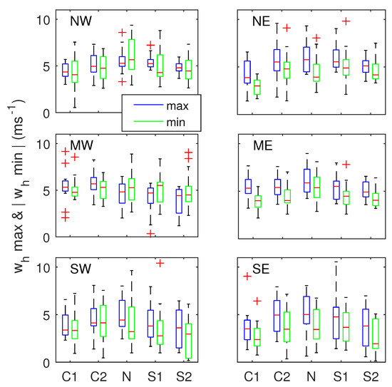
Figure 13.
Box plots of the maximum and minimum (absolute value) vertical wind speed at hub height for different atmospheric stabilities using statistics from the 480 flow fields. The six turbine groups are separated into different subplots. Each box represents samples (representing all combinations of the 4 units per turbine group with 4 initial locations of the cooling source).
5.2. Statistics of Turbine Loads
Based on trends observed in statistics related to the wind velocities, the statistics of turbine loads can also be analyzed according to the same six turbine groups, as is conducted in Figure 14. The extreme load (ExL) extracted from the entire time series is used for all the three load types. All the five stability cases are considered so as to allow comparison of the variation within each turbine group. First, for the OoPBM and FATBM loads, trends appear to be well-correlated with the maximum horizontal wind speed. For example, the mean extreme loads for the same stability in the east groups are higher than those in the west groups because the ambient winds accelerate the outflow. In the convective cases, the SW turbine group experiences higher extreme winds as well as loads compared to those in the neutral and stable cases. Similarly, the SE turbine group experiences the highest extreme winds as well as loads in the neutral case. For the two turbine groups in the middle rows (MW and ME), however, the ExLs for OoPBM and FATBM are not very different among all the stability cases; this is due to the influence of the pitch control system that limits the effect of high winds on loads. Wind speeds in the SW and SE groups are mostly below the rated wind speed of 11.4 m s; due to this, the effect of pitch control is not evident for those groups. Extreme loads in the NW and NE groups are also observed to be limited due to pitch control action. Lower ExL levels in the convective cases due to weaker extreme winds are evident in the OoPBM statistics.
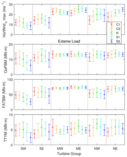
Figure 14.
Statistics of the maximum hub-height wind velocities ( and ) and extreme turbine loads (OoPBM, FATBM, and TTYM) in different stability regimes. The error bars indicate variation over 16 samples (representing all combinations of the 4 units per turbine group with 4 initial locations of the cooling source).
The extreme TTYM loads, again, are observed to be more complex in terms of variability compared to the other two loads; this is due to the sensitivity to asymmetry in the experienced inflow. The yaw moment is also not sensitive to pitch control; hence, TTYM ExL values are not shown to be as effectively reduced as was observed for OoPBM and FATBM (see, especially, the MW and ME groups). Overall, the trend in TTYM extreme load variation is observed to be better correlated with the statistics of the maximum updraft and downdraft. The TTYM ExL is larger in the convective cases for the MW group and larger in the neutral case for all the other turbine groups. Horizontal winds do have some influence on yaw moments; for instance, in the NE group, TTYM ExL values in the stable cases are still observed to be significant, which is consistent with the trend observed in maximum values for that group.
Figure 15 shows box plots of normalized extreme values for the three types of turbine loads (OoPBM, FATBM, and TTYM) and for three stability classes (C1, N, and S2). The entire data set’s mean and standard deviation are computed; then, all the data are shifted and scaled so as to have a zero mean and unit standard deviation. This shift and scale value is then applied to each load type and each stability class for the turbine groups. In this manner, we can compare the uncertainties in each load type as well as across the stability regimes. The SW and SE turbine groups clearly indicate the greatest uncertainty and lowest averages in loads because the outflow is weaker when it passes these turbines. In the middle turbine groups (MW and ME), the OoPBM and FATBM statistics show the least variability arising from the influence of the downburst; this is due to mitigation resulting from pitch control. The TTYM loads are not sensitive to pitch control; hence, their variability even for these turbine groups is still large. The ExL values for the NW and NE turbine groups are also limited by pitch control, but the outflow is not as strong as that along the downburst trajectory. Therefore, the variability in ExL values is lower for these groups compared to that for the south turbine groups but higher than that for the middle turbine groups.
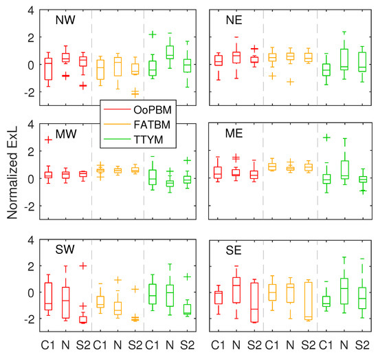
Figure 15.
Box plots of normalized extreme turbine OoPBM, FATBM, and TTYM loads for the C1, N, and S2 cases. Statistics for the six different turbine groups are shown in the different subplots. Each box represents 16 samples (representing all combinations of the 4 units per turbine group with 4 initial locations of the cooling source). The normalization is based on all the data for each load type.
In general, greater variability in extreme loads is observed in the SW and SE turbine groups. Under convective stability (C1) conditions, we observe that there is somewhat greater variability in OoPBM and FATBM extreme loads for the SW group than compared to the SE group. Since the outflow in the SW group is weaker, the ambient turbulence contributes more significantly to the turbine loads and results in the greater uncertainty in the C1 case. The larger uncertainties in the S2 case for the SE group are likely due to fluctuations in the wind direction for the stable case. As noted before, the TTYM extreme loads are a result of other influences such as those from the vertical velocities; hence, the largest uncertainties appear in the neutral case for TTYM ExL.
6. Most Loaded Turbine and Array Risk Assessment
We consider next a scenario where the wind farm is subjected to a strike from a downburst under different atmospheric stabilities. We consider the highest extreme load computed across all the different units in the turbine array and compare this worst-case ExL for the different cases of atmospheric stability. After examination of all the data, the greatest ExL for OoPBM is found to occur in the case C1-0x0y-X9. In Figure 16, we show all the wind turbines in cases C1-0x0y, N-0x0y, and S2-0x0y for comparison, and we indicate the unit that experiences the highest load in the turbine array. The filled circles in the left panels represent the extreme loads at the turbine units by color. Trimmed time series (300–900 s) of the hub-height horizontal wind speed, hub-height horizontal wind direction, pitch angle, and OoPBM load are shown in the right panels for each worst-case turbine.
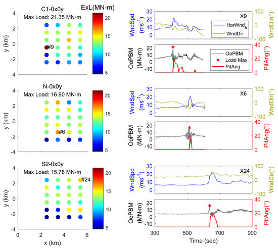
Figure 16.
Time series of hub-height horizontal wind speed, hub-height horizontal wind direction, pitch angle, and turbine load of the worst case with regard to OoPBM ExL in the turbine array for the cases C1-0x0y, N-0x0y, and S2-0x0y (right panels). The locations of the worst-case turbine (most heavily impacted turbine) within the array are also identified in the (left panels), with color bars indicating the ExL level. The ExL values are also shown in the load time series in the (right panels) with a red star marker for each case.
First, we notice that all the worst-case ExL occurrences are at the start time of the triggered pitch control duration which it is very short. These results suggest that it is a rapid increase in horizontal wind speed that causes the identified worst-case load. As observed in the three array plots, units in the southernmost row experience the lowest extreme loads due to the ambient winds deviating toward the northeast, which also causes a drift in the downbursts farther north. The S2 case is accompanied by large deviations in the ambient wind direction. Therefore, it is not surprising that the highest structural demand is felt at the X24 unit. The highest load occurring on X9 in the C1 case is also reasonable to expect since the strength of the outflow decays relatively quickly in the convective ABL. Interestingly, however, this worst-case ExL value for the C1 case of 21.35 MN-m is significantly higher than others for that case, as was noted in the MW panel of Figure 15; it is also significantly greater than the worst-case load for the N and S2 cases. In the neutral case, the highest extreme OoPBM load occurs at unit X6, which is in the SW turbine group.
It is of interest to compare the statistics of the OoPBM extreme loads among all the turbine groups, as is performed in Figure 14. Generally speaking, these extreme loads are observed to be higher for groups in the middle rows and the north rows. The highest extreme load among all the turbines in the array, however, tends to occur under a situation resulting from greater uncertainties, such as observed with the SW and SE groups. Turbine groups that experience strong outflows are in fact well-protected by the pitch control action and, thus, avoid experiencing the highest extreme load. In an earlier study of wind farm risks using a stochastic downburst model [40], the worst-case load in a wind farm was always found to occur at the end time of pitch control period, which is not consistent with our results using LES-generated downbursts. This could be attributed to differences in the extent and duration of the rapid increase in the downburst surge. Moreover, the increase in outflow wind speeds in the stochastic model primarily follows the trend of the mean wind field and not the fluctuating turbulent wind. Superimposed stochastic turbulence is likely too weak to simulate realistic wind surges. The rapid changes in wind direction might also have been underestimated. The FAST turbine response simulations in the worst-case scenarios for the C1 and N cases are actually terminated due to turbulent winds after the maximum outflow occurs; no similar case was reported in the work of Nguyen et al. [40].
The largest single turbine extreme FATBM load is found in case S1-0x0y-X12. In Figure 17, we present the time series of horizontal winds and this turbine’s FATBM load, as well as the distribution of FATBM ExL values over the entire turbine array. The cases C1-0x0y and N-0x0y are also shown for comparison. Similar to what we observed with the OoPBM loads, the largest FATBM loads occur at or near the start time of the pitch control duration, which is very short. The variability in FATBM loads is smaller (than for OoPBM); hence, the worst-case FATBM ExL is not observed to be an outlier relative to other cases for C1 (see the ME group for C1 in Figure 14 that includes unit X12). For all the turbines, FATBM extreme loads are in the range of about 60–80 MN-m. The location of the worst-case turbine’s extreme load is, for all stability cases, in the rightmost column ( km), which is favorable for the primary surge with a short time span since the sustained winds are less intense when the ring vortex reaches here. For the C1 case, the largest FATBM ExL occurs at unit X20, compared to the largest OoPBM load that occurs at unit X9 for C1 stability. After examination of the loads on these two distinct and spatially separated turbine units, we note that the rapid increase in wind speed in C1 (convective) stability at these locations, X9 and X20, places them at risk under both extreme levels of OoPBM and FATBM, although they do not occur at the same time during the downburst. The FATBM ExL level on unit X9 does not occur at the start time of the pitch control action and, therefore, has a lower ExL value at the time when its OoPBM is largest.
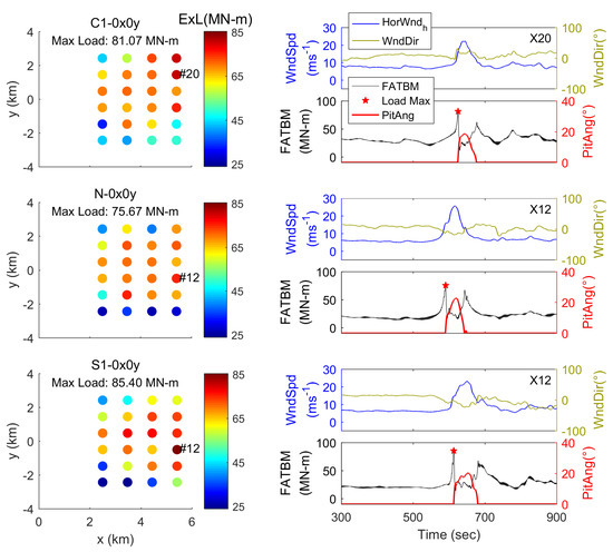
Figure 17.
Time series of hub-height horizontal wind speed, hub-height horizontal wind direction, pitch angle, and turbine load of the worst case with regard to FATBM ExL in the turbine array for the cases C1-0x0y, N-0x0y, and S2-0x0y (right panels). The locations of the worst-case turbine (most heavily impacted turbine) within the array are also identified in the (left panels), with color bars indicated the ExL level. The ExL values are also shown in the load time series in the (right panels) with a red star marker for each case.
The largest single-turbine extreme TTYM load is also analyzed, as was conducted with the other loads (OoPBM and FATBM). The case C1-0x0y in which the worst-case extreme yaw moment occurs is presented in Figure 18 together with the other two cases, N-0x0y and S2-0x0y. Here, we present the time series of the hub-height vertical wind speed and yaw error instead of wind direction in order to better assess a connection with the time series of the TTYM load. Since the yaw moment has been noted to exhibit greater variability compared to the other two load types, the worst-case largest TTYM loads are seen to be significantly greater for the one turbine than for all the other turbines in the array (for instance, for X9, compared to all other turbines in C1 stability). As can be observed, the extreme TTYM loads are observed to be directly related to the maximum outflow. The maximum horizontal wind speed, on its own, does not directly influence the TTYM ExL; this is due to mitigation from pitch control action. The largest TTYM load peak occurs at a time when the updraft turns to a downdraft, which results from the impact of the ring vortex and creates large asymmetric loading on the turbine blades. The yaw error is not observed to be very clearly related to the TTYM ExL, but it is expected to have an influence on larger fluctuations in TTYM after the impact of the outflow. Based on our investigations, larger yaw errors after the maximum outflow can sometimes result in extreme loads, especially for units X13 and X14 (MW group) in the stable cases, but the resulting TTYM ExL levels are found to be much smaller than those caused by the direct impact of the ring vortex.
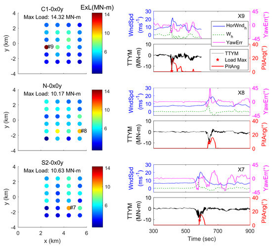
Figure 18.
Time series of hub-height horizontal wind speed, hub-height vertical wind speed, yaw error, pitch angle, and turbine load of the worst case with regard to TTYM ExL in the turbine array for the cases C1-0x0y, N-0x0y, and S2-0x0y (right panels). The locations of the worst-case turbine (most heavily impacted turbine) within the array are also identified in the (left panels), with color bars indicated the ExL level. The ExL values are also shown in the load time series in the (right panels) with a red star marker for each case.
Figure 19 shows a comparison of the array-average maximum hub-height wind speed and extreme turbine loads from each of the 20 LES runs, resulting from four different cooling source locations and five different atmospheric stability cases. By array-average extreme, we mean that we are no longer considering the worst-case extreme among all units but instead average the extreme values over all the 24 units in the array; accordingly, an array-average OoPBM ExL, for instance, refers to the average of OoPBM ExL values over all 24 turbines. Here, we examine the array-average extreme wind speed and loads in order to investigate the overall characteristics of the entire array. The relationships between maximum wind velocities and extreme loads for the individual inflow fields and turbines, as well as the interplay with atmospheric stability conditions are shown in Figure 14. From the statistics of the maximum wind speed, the neutral case clearly shows the most systematic largest mean among all the cases (the weakly convective case, C2, also experiences comparable wind speed levels, although the pattern is not as consistent). This can be explained by the dissipated ring vortex which causes larger winds in the convective cases closer to the touchdown location but larger winds in the stable cases for fields farther away from the touchdown, as was noted in Figure 12. The array-average extreme OoPBM and TTYM loads are observed to be strongly correlated with the maximum wind speed; for the FATBM loads, a clearer trend is evident where these loads decrease as the stability increases. A reason for this observation can be understood by comparing Figure 16 and Figure 17. In the C1 case, the extreme OoPBM is observed to decrease as the ring vortex propagates and dissipates (away from the touchdown), whereas the extreme FATBM is observed to be large because the short time span of the outflow surge can still result in high ExL values. Therefore, the array-average ExL for FATBM appears to be greater in the convective cases. Note that a larger worst-case FATBM load can occur in a stable case (say S1), as discussed before, but the array-average extreme load will be lower due to the deviated ambient winds that decrease these turbine loads (especially in the southernmost row) to a certain extent.
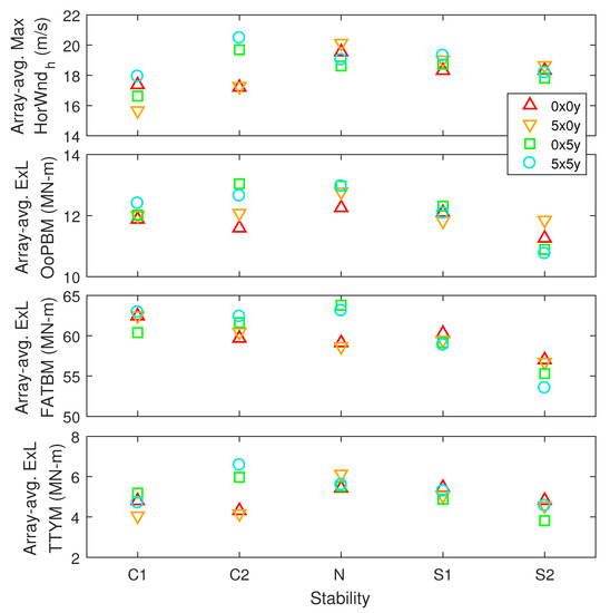
Figure 19.
Comparison of array-average hub-height maximum wind speed and extreme turbine loads for the data from the 20 LES runs. Samples with four different cooling source locations are denoted by different markers.
From a risk assessment perspective, the preceding discussion highlights the influence in both a worst-case sense—i.e., for the maximum damage a single turbine might experience—as well as in an average sense of how thunderstorm downbursts are felt across a turbine array. The structural demands on the turbine tower, blades, and nacelle are different, and hence the risk of failure varies with location of each turbine relative to initiation cooling source locations and related touchdown points. The characteristics of the wind field and the systems for pitch and yaw control as well as the time-varying changes in the wind velocity components and wind direction all influence the experienced risks.
7. Conclusions
In the present study, an LES-ABL framework for the simulation of idealized downbursts initiated using a cooling source in different stability regimes is presented. The generated full-domain wind fields are applied to a rectilinear turbine array with 3-D inflow fields extracted at the locations of each of the turbine units. The characteristics of the inflow field and associated loads at each turbine are investigated in detail. The influence of atmospheric stability is studied through statistical analyses of the wind velocity and extreme loads from all the data sets. Worst-case scenarios for each load type are also compared among the selected cases with different stabilities.
Investigations on the wind structure reveal that the evolution and state of maturity of the ring vortex play an important role in the characteristics of the outflow. Since a strong outflow band forms more slowly as atmospheric stability increases, the downdraft, updraft, and extreme outflow are expected to appear strongest in the convective case. However, this is consistent with our findings only when the flow fields are close to the touchdown center. This is due to the dissipation of the ring vortex and interaction with ambient winds. In the convective boundary layer, the strength of the outflow decays much sooner than that in stable atmospheric environments. Thus, it is observed that the levels of the maximum horizontal wind speed at the hub height for turbine groups farther from the touchdown locations are lower in the convective cases. Since the ambient winds tend to deviate the flow fields more systematically toward the northeast as the stability increases, the horizontal winds in the most stable case (S2) are observed to be the strongest for the northeast turbine group. The statistics of the vertical wind velocity are also found to be related to the dissipation of the ring vortex and interaction with the ambient winds.
Extreme OoPBM and FATBM loads are found to be dependent on the extreme winds but are mitigated by pitch control action, especially in the turbine groups close to or along the downburst track. Compared to OoPBM and FATBM, the TTYM ExL exhibits greater variability for all the turbine groups. TTYM loads are not sensitive to pitch control action but are affected by vertical velocities. In general, the outflow of a downburst is observed to more significantly impact turbines farther away from the touchdown center in the stable cases, especially when the ambient winds are aligned with the downburst. The worst loads on the wind turbine array also occur on units farther from the center for those stable cases.
Future work could focus on the downburst impacts on a wind farm while taking into consideration wake effects within the turbine array. Here, we placed greater emphasis on the role of atmospheric stability and its influence on flow fields in a downburst and associated turbine extreme loads over the entire wind farm. It would be useful to consider wake effects on the turbine units, even though it is likely that wakes are less organized during extreme winds associated with downbursts. We note that the LES model employed here, while it includes ABL physics important in simulating thunderstorm downbursts, still falls short in the consideration of other realistic atmospheric parameters. Future work might consider including parameterizations of other microphysics in the LES model and coupling with mesoscale models (e.g., WRF) in order to approach more realistic conditions.
Author Contributions
Conceptualization, L.M. and S.B.; methodology, L.M. and S.B.; software, S.B., P.H. and N.-Y.L.; validation, P.H. and N.-Y.L.; writing—original draft preparation, N.-Y.L.; writing—review and editing, N.-Y.L., L.M., P.H. and S.B.; funding acquisition, L.M. and S.B. All authors have read and agreed to the published version of the manuscript.
Funding
This material is based upon work supported by the National Science Foundation under Grant Nos. 1336304 and 1336760. The authors are grateful for this support. Any opinions, findings, and conclusions or recommendations expressed in this material are those of the authors and do not necessarily reflect the views of the National Science Foundation.
Institutional Review Board Statement
Not applicable.
Informed Consent Statement
Not applicable.
Acknowledgments
The authors are grateful to the Texas Advanced Computing Center (TACC [51]) at The University of Texas at Austin for providing high-performance computing (HPC) resources that have contributed to the research results reported within this paper. All the turbine load simulations as well as the associated inflow generation are carried out in the Stampede2 supercomputer at the TACC. URL: http://www.tacc.utexas.edu, accessed on 24 August 2021.
Conflicts of Interest
The authors declare no conflict of interest.
Abbreviations
The following abbreviations are used in this manuscript:
| ET | Evening transition |
| ABL | Atmospheric boundary layer |
| CBL | Convective boundary layer |
| SBL | Stable boundary layer |
| LES | Large-eddy simulation |
| C1 | Convective condition |
| C2 | Weakly convective condition |
| N | Near-neutral condition |
| S1 | Weakly stable condition |
| S2 | Stable condition |
| SW | Southwest turbine group |
| SE | Southeast turbine group |
| MW | Middle-west turbine group |
| ME | Middle-east turbine group |
| NW | Northwest turbine group |
| NE | Northeast turbine group |
| OoPBM | Blade root out-of-plane bending moment |
| FATBM | Fore-aft tower bending moment |
| TTYM | Tower-top yaw moment |
| BEM | Blade element momentum |
| GDW | Generalized dynamic wake |
| ExL | Extreme load |
| AGL | Above ground level |
References
- Fujita, T. The Downburst; SMRP Research Paper Number 210; Department of the Geophysical Sciences, The University of Chicago: Chicago, IL, USA, 1985. [Google Scholar]
- Fujita, T. Downbursts: Meteorological features and wind field characteristics. J. Wind. Eng. Ind. Aerodyn. 1990, 36, 75–86. [Google Scholar] [CrossRef]
- Hawes, H. Review of recent Australian transmission line failures due to high intensity winds. In Proceedings of the Report to Task Force on High Intensity Winds on Transmission Lines, Buenos Aires, Argentina, 19–23 April 1993. [Google Scholar]
- Holmes, J. Modeling of extreme thunderstorm winds for wind loading of structures and risk assessment. In Proceedings of the Tenth International Conference on Wind Engineering, Copenhagen, Denmark, 21–24 June 1999; pp. 1409–1415. [Google Scholar]
- Hawbecker, P.; Basu, S.; Manuel, L. Realistic simulations of the July 1, 2011 severe wind event over the Buffalo Ridge wind farm. Wind Energy 2017, 20, 1803–1822. [Google Scholar] [CrossRef]
- Hawbecker, P.; Basu, S.; Manuel, L. Investigating the impact of atmospheric stability on thunderstorm outflow winds and turbulence. Wind Energy Sci. 2018, 3, 203. [Google Scholar] [CrossRef] [Green Version]
- Stull, R. An Introduction to Boundary Layer Meteorology; Springer Science & Business Media: Berlin/Heidelberg, Germany, 2012; Volume 13. [Google Scholar]
- Vicroy, D. A Simple, Analytical, Axisymmetric Microburst Model for Downdraft Estimation; Technical Report, NASA Report TM 104053; NASA: Washington, DC, USA, 1991. [Google Scholar]
- Chay, M.; Albermani, F.; Wilson, R. Numerical and analytical simulation of downburst wind loads. Eng. Struct. 2006, 28, 240–254. [Google Scholar] [CrossRef] [Green Version]
- Nguyen, H.; Manuel, L.; Veers, P. Wind turbine loads during simulated thunderstorm microbursts. J. Renew. Sustain. Energy 2011, 3, 053104. [Google Scholar] [CrossRef]
- Anabor, V.; Rizza, U.; Nascimento, E.; Degrazia, G. Large-eddy simulation of a microburst. Atmos. Chem. Phys. 2011, 11, 9323–9331. [Google Scholar] [CrossRef] [Green Version]
- Vermeire, B.; Orf, L.; Savory, E. Improved modelling of downburst outflows for wind engineering applications using a cooling source approach. J. Wind. Eng. Ind. Aerodyn. 2011, 99, 801–814. [Google Scholar] [CrossRef]
- Orf, L.; Kantor, E.; Savory, E. Simulation of a downburst-producing thunderstorm using a very high-resolution three-dimensional cloud model. J. Wind. Eng. Ind. Aerodyn. 2012, 104, 547–557. [Google Scholar] [CrossRef]
- Aboshosha, H.; Bitsuamlak, G.; Damatty, A.E. Turbulence characterization of downbursts using LES. J. Wind. Eng. Ind. Aerodyn. 2015, 136, 44–61. [Google Scholar] [CrossRef]
- Haines, M.; Taylor, I. Numerical investigation of the flow field around low rise buildings due to a downburst event using large eddy simulation. J. Wind. Eng. Ind. Aerodyn. 2018, 172, 12–30. [Google Scholar] [CrossRef] [Green Version]
- Anderson, W.; Basu, S.; Letchford, C. Comparison of dynamic subgrid-scale models for simulations of neutrally buoyant shear-driven atmospheric boundary layer flows. Environ. Fluid Mech. 2007, 7, 195–215. [Google Scholar] [CrossRef]
- Anderson, J.; Orf, L.; Straka, J. A 3-D model system for simulating thunderstorm microburst outflows. Meteorol. Atmos. Phys. 1992, 49, 125–131. [Google Scholar] [CrossRef]
- Oliver, S.; Moriarty, W.; Holmes, J. A risk model for design of transmission line systems against thunderstorm downburst winds. Eng. Struct. 2000, 22, 1173–1179. [Google Scholar] [CrossRef]
- Li, C. A stochastic model of severe thunderstorms for transmission line design. Probabilistic Eng. Mech. 2000, 15, 359–364. [Google Scholar] [CrossRef]
- Savory, E.; Parke, G.; Zeinoddini, M.; Toy, N.; Disney, P. Modelling of tornado and microburst-induced wind loading and failure of a lattice transmission tower. Eng. Struct. 2001, 23, 365–375. [Google Scholar] [CrossRef]
- Chen, L.; Letchford, C. A deterministic–stochastic hybrid model of downbursts and its impact on a cantilevered structure. Eng. Struct. 2004, 26, 619–629. [Google Scholar] [CrossRef]
- Chen, L.; Letchford, C. Parametric study on the along-wind response of the CAARC building to downbursts in the time domain. J. Wind. Eng. Ind. Aerodyn. 2004, 92, 703–724. [Google Scholar] [CrossRef]
- Solari, G. Thunderstorm response spectrum technique: Theory and applications. Eng. Struct. 2016, 108, 28–46. [Google Scholar] [CrossRef]
- Le, T.; Caracoglia, L. Modeling vortex-shedding effects for the stochastic response of tall buildings in non-synoptic winds. J. Fluids Struct. 2016, 61, 461–491. [Google Scholar] [CrossRef] [Green Version]
- Le, T.; Caracoglia, L. Computer-based model for the transient dynamics of a tall building during digitally simulated Andrews AFB thunderstorm. Comput. Struct. 2017, 193, 44–72. [Google Scholar] [CrossRef]
- Miguel, L.; Riera, J.; Miguel, L. Assessment of downburst wind loading on tall structures. J. Wind. Eng. Ind. Aerodyn. 2018, 174, 252–259. [Google Scholar] [CrossRef]
- Chay, M.; Letchford, C. Pressure distributions on a cube in a simulated thunderstorm downburst? Part A: Stationary downburst observations. J. Wind. Eng. Ind. Aerodyn. 2002, 90, 711–732. [Google Scholar] [CrossRef]
- Letchford, C.; Chay, M. Pressure distributions on a cube in a simulated thunderstorm downburst. Part B: Moving downburst observations. J. Wind. Eng. Ind. Aerodyn. 2002, 90, 733–753. [Google Scholar] [CrossRef]
- Sarkar, P.; Haan, F., Jr.; Balaramudu, V.; Sengupta, A. Laboratory simulation of tornado and microburst to assess wind loads on buildings. In Proceedings of the Structures Congress 2006: Structural Engineering and Public Safety, St. Louis, MO, USA, 18–21 May 2006; pp. 1–10. [Google Scholar]
- Zhang, Y.; Sarkar, P.; Hu, H. An experimental study of flow fields and wind loads on gable-roof building models in microburst-like wind. Exp. Fluids 2013, 54, 1–21. [Google Scholar] [CrossRef]
- Zhang, Y.; Hu, H.; Sarkar, P. Comparison of microburst-wind loads on low-rise structures of various geometric shapes. J. Wind. Eng. Ind. Aerodyn. 2014, 133, 181–190. [Google Scholar] [CrossRef]
- Zhang, Y.; Sarkar, P.; Hu, H. An experimental study on wind loads acting on a high-rise building model induced by microburst-like winds. J. Fluids Struct. 2014, 50, 547–564. [Google Scholar] [CrossRef]
- Zhang, Y.; Sarkar, P.; Hu, H. An experimental investigation on the characteristics of fluid–structure interactions of a wind turbine model sited in microburst-like winds. J. Fluids Struct. 2015, 57, 206–218. [Google Scholar] [CrossRef]
- Shehata, A.; Damatty, A.E.; Savory, E. Finite element modeling of transmission line under downburst wind loading. Finite Elem. Anal. Des. 2005, 42, 71–89. [Google Scholar] [CrossRef]
- Al-Issa, A.; Ansary, A.E.; Aboshosha, H.; Aboutabikh, M.; Ghazal, T. Evaluation of peak transmission line conductor reactions under downburst winds using optimization and simplified approaches. Front. Built Environ. 2019, 5, 88. [Google Scholar] [CrossRef]
- Sengupta, A.; Haan, F.; Sarkar, P.; Balaramudu, V. Transient loads on buildings in microburst and tornado winds. J. Wind. Eng. Ind. Aerodyn. 2008, 96, 2173–2187. [Google Scholar] [CrossRef]
- Sim, T.; Ong, M.; Quek, W.; Sum, Z.; Lai, W.; Skote, M. A numerical study of microburst-like wind load acting on different block array configurations using an impinging jet model. J. Fluids Struct. 2016, 61, 184–204. [Google Scholar] [CrossRef]
- Hao, J.; Wu, T. Downburst-induced transient response of a long-span bridge: A CFD-CSD-based hybrid approach. J. Wind. Eng. Ind. Aerodyn. 2018, 179, 273–286. [Google Scholar] [CrossRef]
- Lu, N.-Y.; Hawbecker, P.; Basu, S.; Manuel, L. On wind turbine loads during thunderstorm downbursts in contrasting atmospheric stability regimes. Energies 2019, 12, 2773. [Google Scholar] [CrossRef] [Green Version]
- Nguyen, H.; Manuel, L. Thunderstorm downburst risks to wind farms. J. Renew. Sustain. Energy 2013, 5, 013120. [Google Scholar] [CrossRef]
- Park, J.; Basu, S.; Manuel, L. Large-eddy simulation of stable boundary layer turbulence and estimation of associated wind turbine loads. Wind Energy 2014, 17, 359–384. [Google Scholar] [CrossRef]
- Lu, N.-Y.; Basu, S.; Manuel, L. On wind turbine loads during the evening transition period. Wind Energy 2019, 22, 1288–1309. [Google Scholar] [CrossRef]
- Basu, S.; Portė-Agel, F. Large-eddy simulation of stably stratified atmospheric boundary layer turbulence: A scale-dependent dynamic modeling approach. J. Atmos. Sci. 2006, 63, 2074–2091. [Google Scholar] [CrossRef] [Green Version]
- Orf, L.; Anderson, J.; Straka, J. A three-dimensional numerical analysis of colliding microburst outflow dynamics. J. Atmos. Sci. 1996, 53, 2490–2511. [Google Scholar] [CrossRef] [Green Version]
- Jeon, M.; Lee, S.; Kim, T.; Lee, S. Wake influence on dynamic load characteristics of offshore floating wind turbines. AIAA J. 2016, 54, 3535–3545. [Google Scholar] [CrossRef]
- Jonkman, J.; Butterfield, S.; Musial, W.; Scott, G. Definition of a 5MW Reference Wind Turbine for Offshore System Development; National Renewable Energy Laboratory Technical Report NREL/TP-500-38060; National Renewable Energy Laboratory: Golden, CO, USA, 2007. [Google Scholar]
- Jonkman, J.; Buhl, M. FAST User’s Guide; National Renewable Energy Laboratory Technical Report NREL/EL-500-38230; National Renewable Energy Laboratory: Golden, CO, USA, 2005. [Google Scholar]
- Suzuki, A. Application of Dynamic Inflow Theory to Wind Turbine Rotors. Ph.D. Thesis, The University of Utah, Salt Lake City, UT, USA, 2001. [Google Scholar]
- Nguyen, H.; Manuel, L.; Jonkman, J.; Veers, P.S. Simulation of thunderstorm downbursts and associated wind turbine loads. J. Sol. Energy Eng. 2013, 135, 021014. [Google Scholar] [CrossRef]
- Nguyen, H.; Manuel, L. Extreme and fatigue loads on wind turbines during thunderstorm downbursts: The influence of alternative turbulence models. J. Renew. Sustain. Energy 2015, 7, 013102. [Google Scholar] [CrossRef]
- Koziol, Q. High Performance Parallel I/O; Chapter 7: Texas Advanced Computing Center; Chapman and Hall/CRC: Boca Raton, FL, USA, 2014. [Google Scholar]
Publisher’s Note: MDPI stays neutral with regard to jurisdictional claims in published maps and institutional affiliations. |
© 2021 by the authors. Licensee MDPI, Basel, Switzerland. This article is an open access article distributed under the terms and conditions of the Creative Commons Attribution (CC BY) license (https://creativecommons.org/licenses/by/4.0/).