
Associating Synoptic-Scale Weather Patterns with Aggregated Offshore Wind Power Production and Ramps


Abstract
:1. Introduction
2. Data
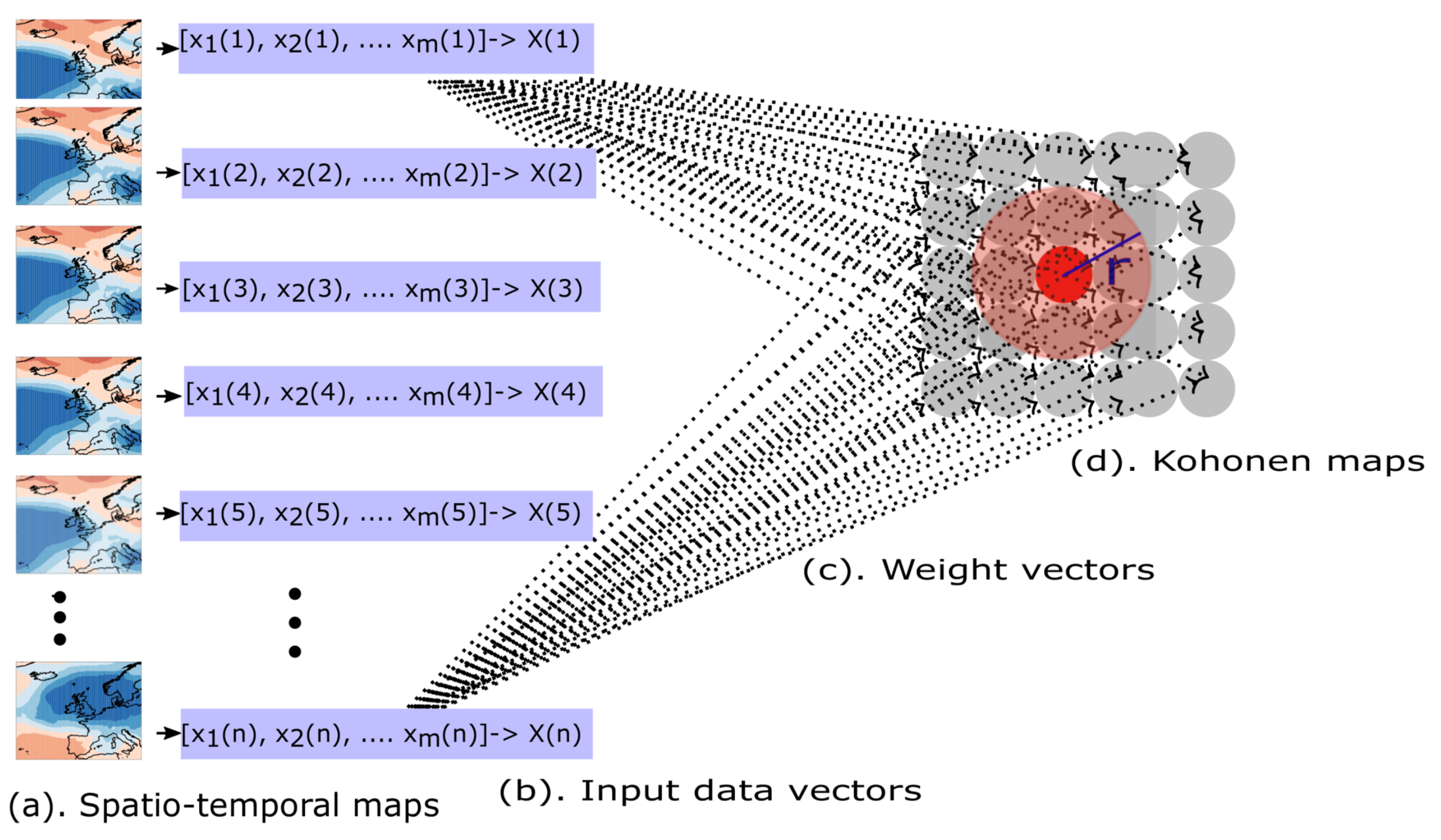
3. Methods
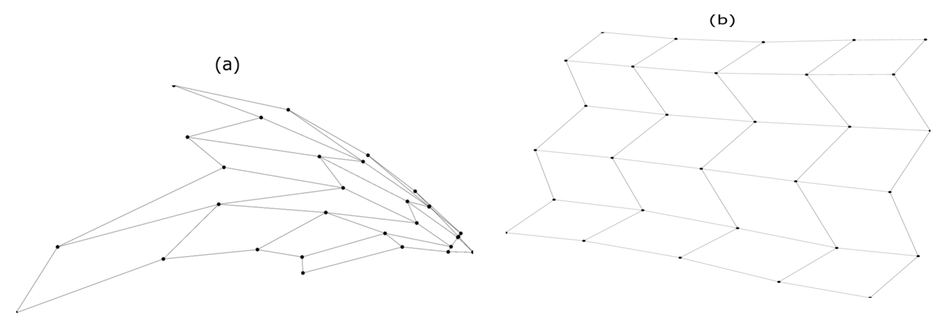
3.1. SOM Algorithm
3.2. Detecting Wind Power Ramps
4. Results
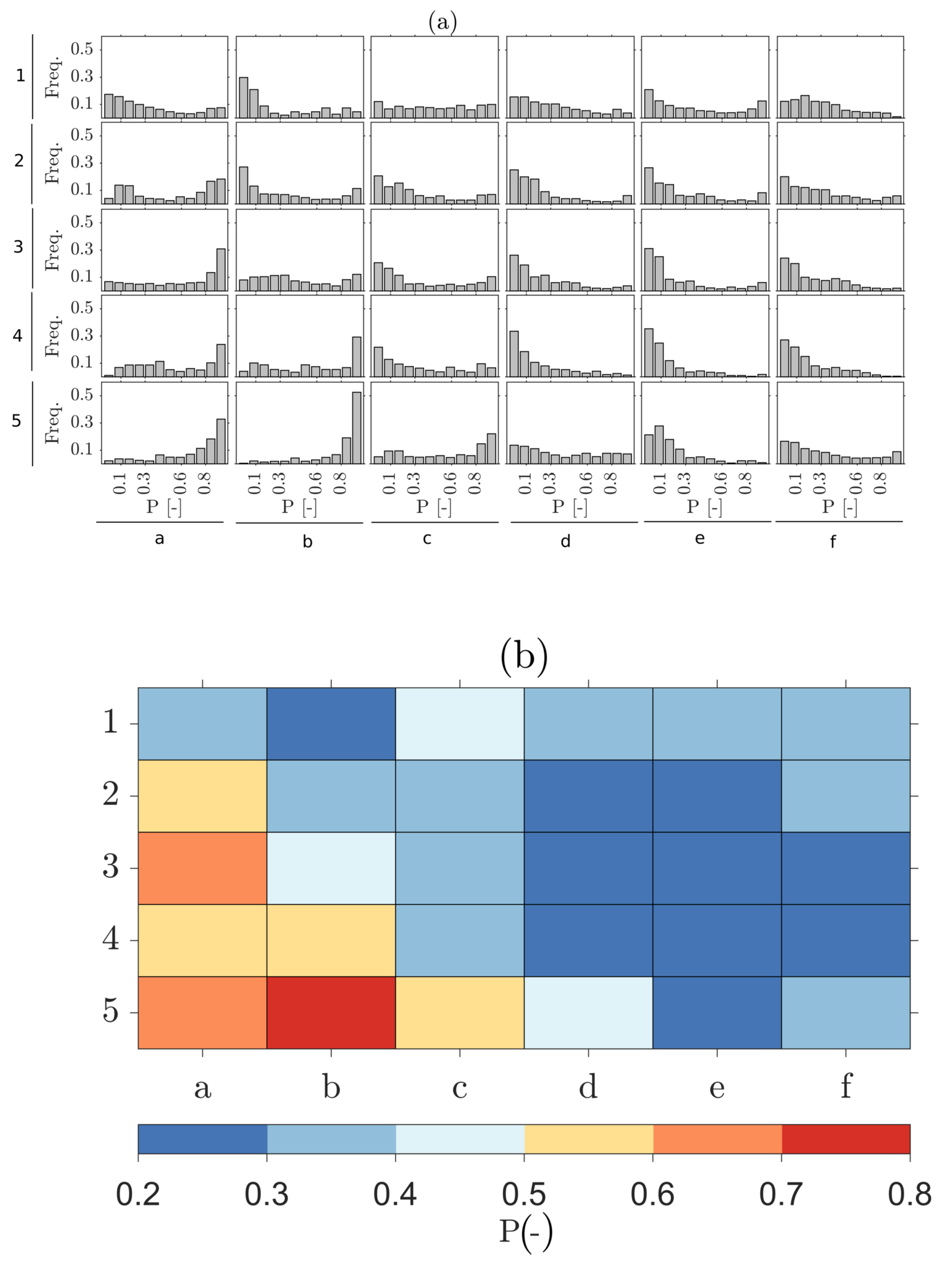
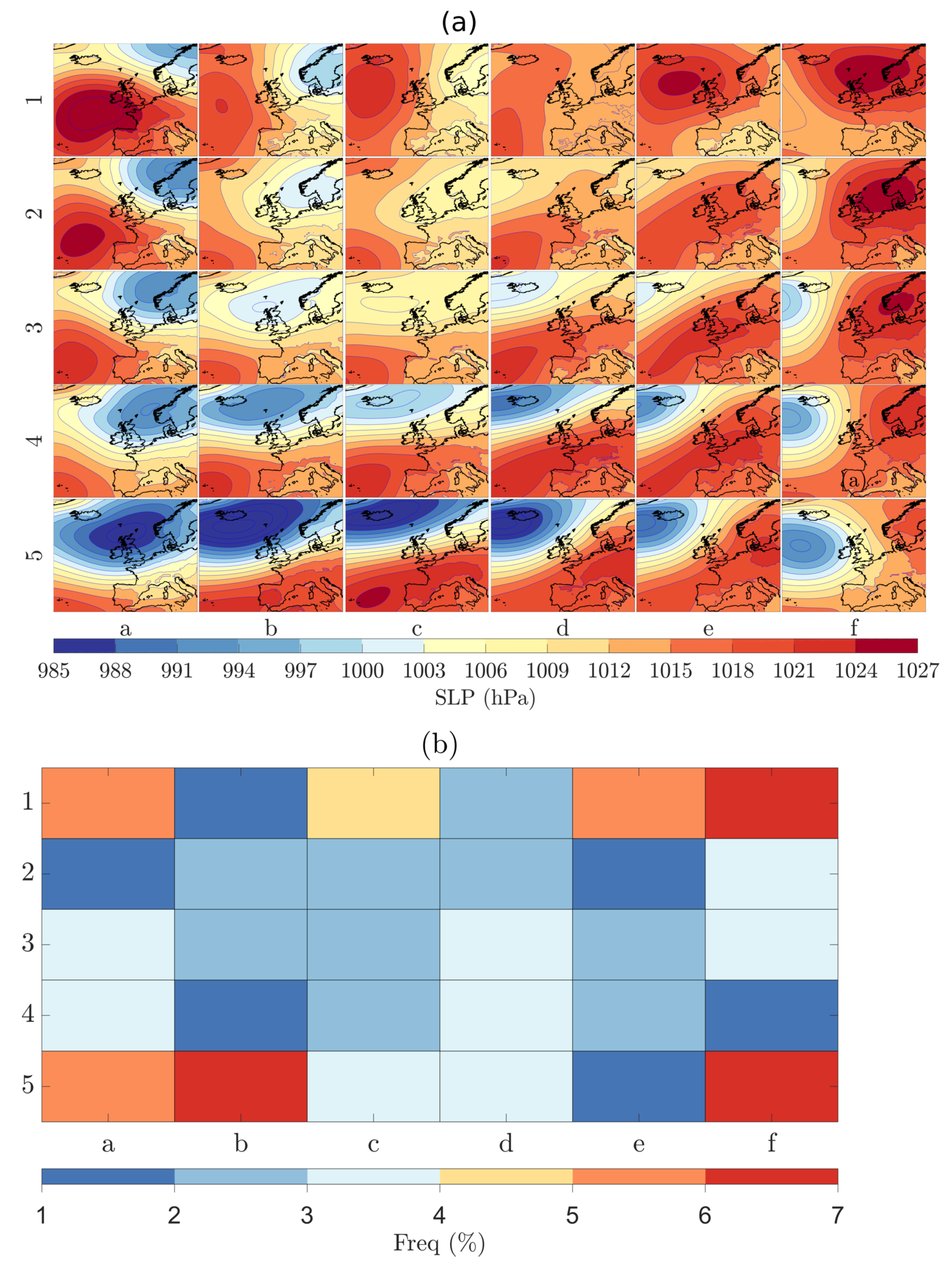
4.1. Weather Patterns
4.2. Wind Power Trends by Weather Pattern
4.2.1. Wind Power Production
4.2.2. Wind Power Ramps
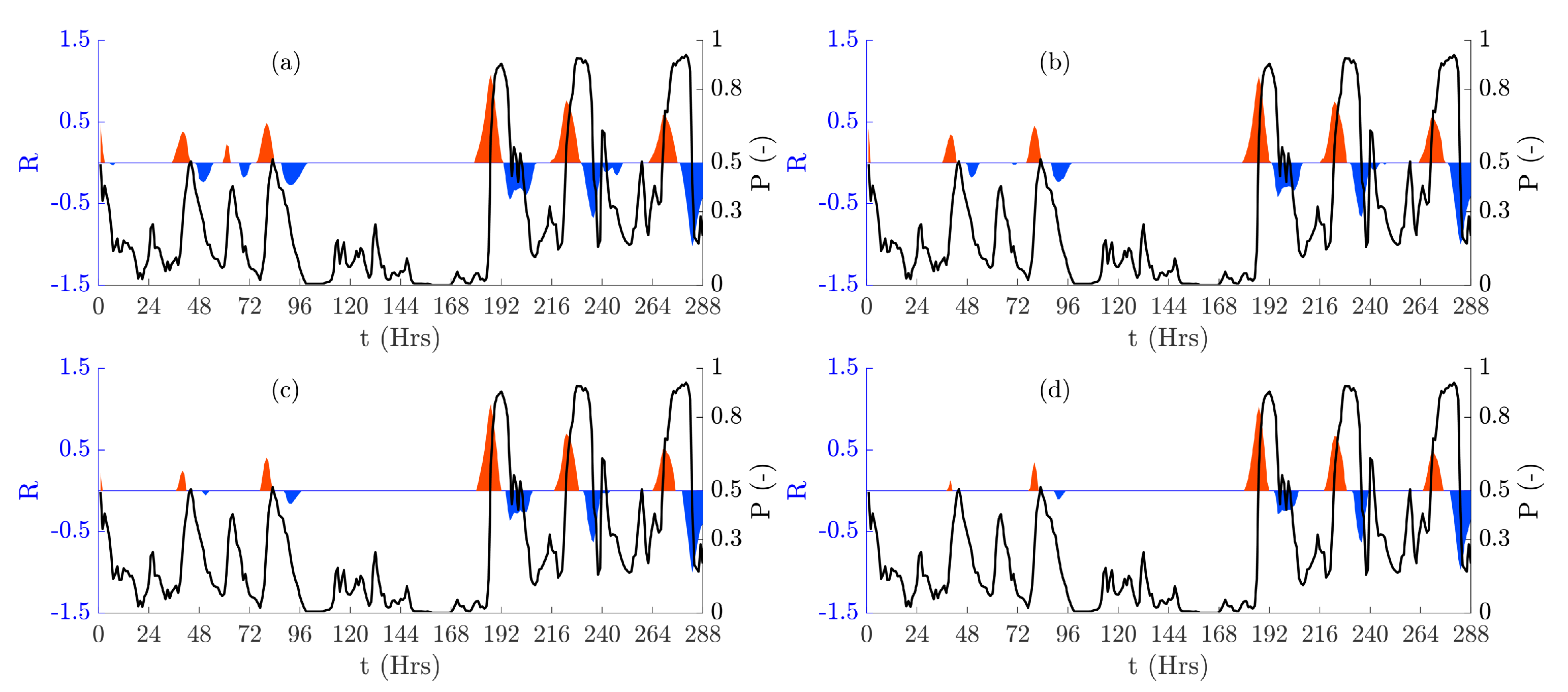
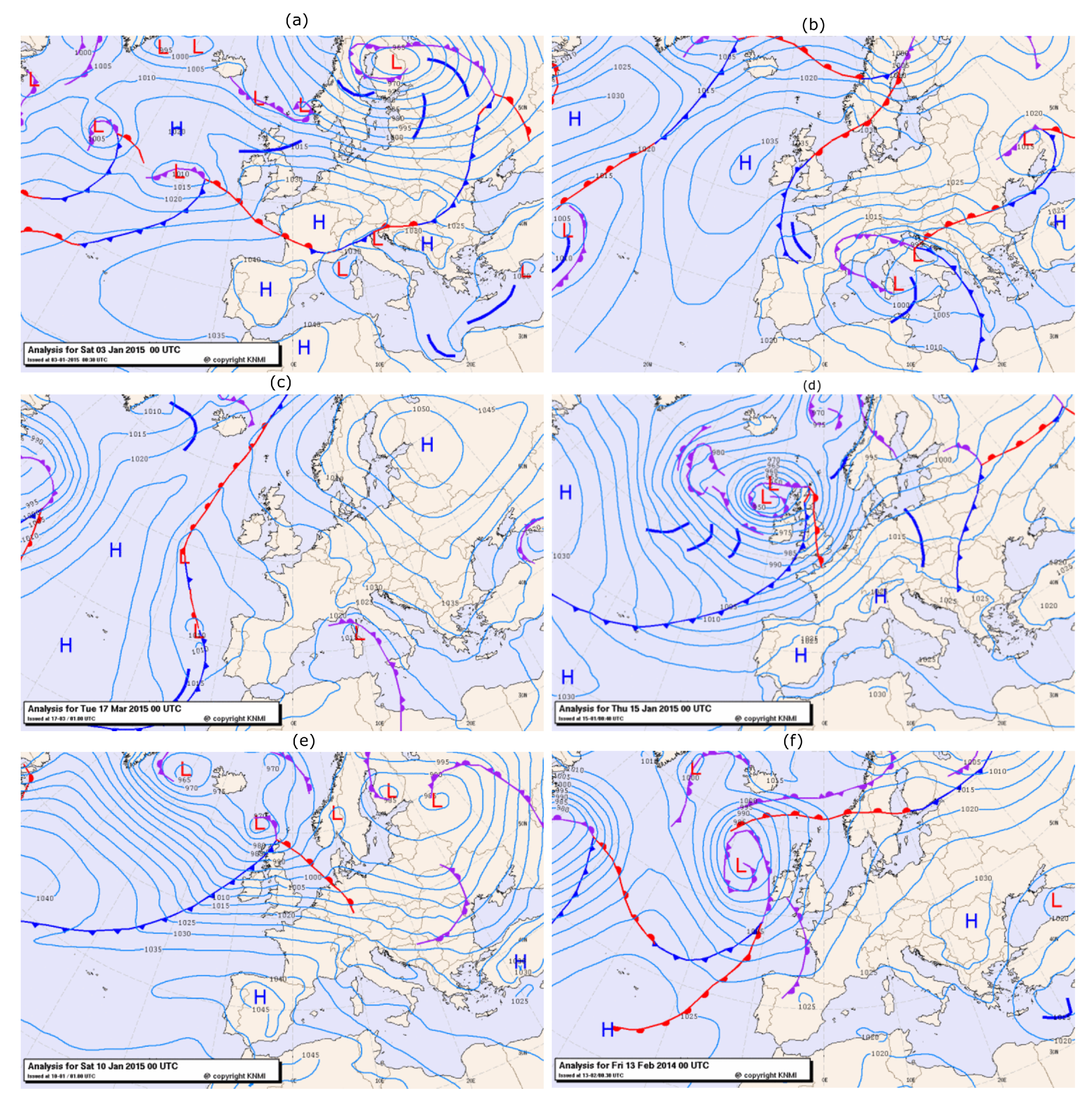
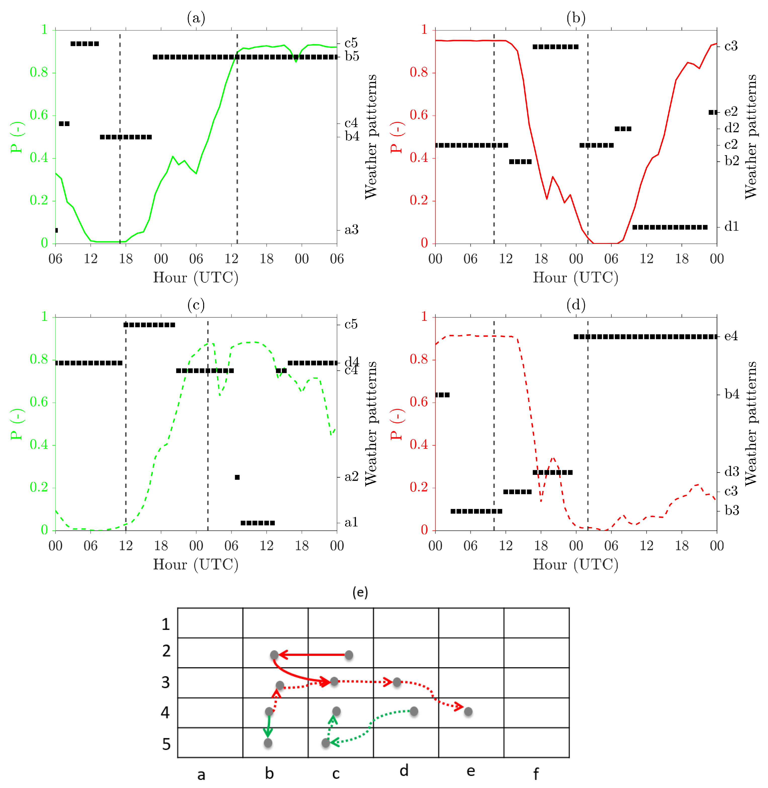
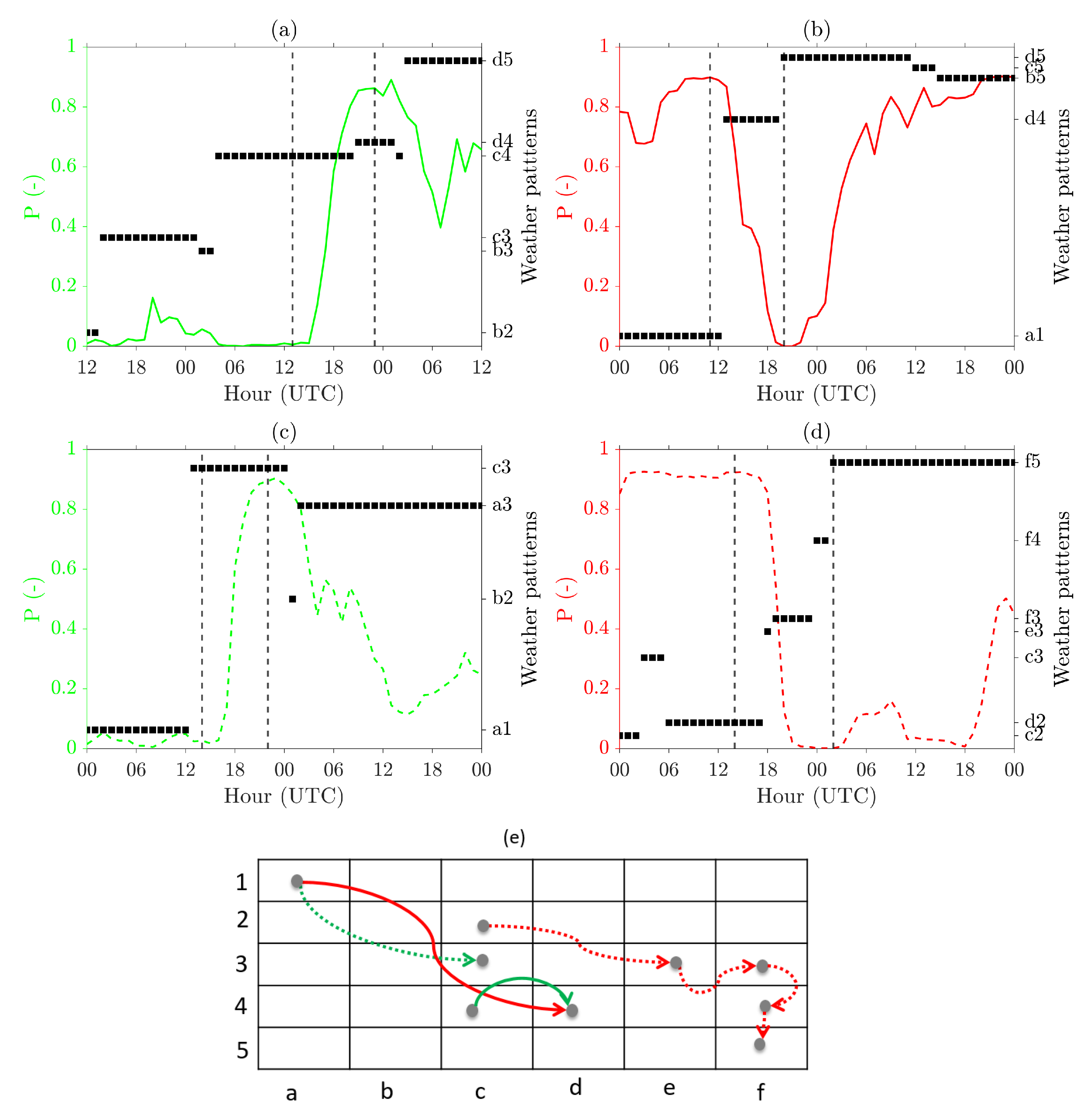
4.2.3. Wind Power Ramp Case Studies
5. Conclusions
Author Contributions
Funding
Institutional Review Board Statement
Informed Consent Statement
Data Availability Statement
Conflicts of Interest
References
- WindEurope. 2020 Statistics and the Outlook for 2021–2025; Published in February 2021; WindEurope: Brussels, Belgium, 2021. [Google Scholar]
- WindEurope. Wind Energy in Europe: Scenarios for 2030; WindEurope: Brussels, Belgium, 2017. [Google Scholar]
- Orlanski, I. A rational subdivision of scales for atmospheric processes. Bull. Am. Meteorol. Soc. 1975, 56, 527–530. [Google Scholar]
- Fujita, T.T. Tornadoes and downbursts in the context of generalized planetary scales. J. Atmos. Sci. 1981, 38, 1511–1534. [Google Scholar] [CrossRef] [Green Version]
- Fujita, T. Mesoscale classifications: Their history and their application to forecasting. In Mesoscale Meteorology and Forecasting; Springer: Berlin/Heisenberg, Germany, 1986; pp. 18–35. [Google Scholar]
- Emanuel, K.A. Overview and definition of mesoscale meteorology. In Mesoscale Meteorology and Forecasting; Springer: Berlin, Germany, 1986; pp. 1–17. [Google Scholar]
- Thunis, P.; Bornstein, R. Hierarchy of mesoscale flow assumptions and equations. J. Atmos. Sci. 1996, 53, 380–397. [Google Scholar] [CrossRef]
- Brayshaw, D.J.; Troccoli, A.; Fordham, R.; Methven, J. The impact of large scale atmospheric circulation patterns on wind power generation and its potential predictability: A case study over the UK. Renew. Energy 2011, 36, 2087–2096. [Google Scholar] [CrossRef]
- Correia, J.; Bastos, A.; Brito, M.; Trigo, R. The influence of the main large-scale circulation patterns on wind power production in Portugal. Renew. Energy 2017, 102, 214–223. [Google Scholar] [CrossRef]
- Grams, C.M.; Beerli, R.; Pfenninger, S.; Staffell, I.; Wernli, H. Balancing Europe’s wind power output through spatial deployment informed by weather regimes. Nat. Clim. Chang. 2017, 7, 557–562. [Google Scholar] [CrossRef] [PubMed] [Green Version]
- Thornton, H.E.; Scaife, A.A.; Hoskins, B.J.; Brayshaw, D.J. The relationship between wind power, electricity demand and winter weather patterns in Great Britain. Environ. Res. Lett. 2017, 12, 064017. [Google Scholar] [CrossRef]
- Cradden, L.C.; McDermott, F. A weather regime characterisation of Irish wind generation and electricity demand in winters 2009–11. Environ. Res. Lett. 2018, 13, 054022. [Google Scholar] [CrossRef]
- Drew, D.R.; Barlow, J.F.; Coker, P.J. Identifying and characterising large ramps in power output of offshore wind farms. Renew. Energy 2018, 127, 195–203. [Google Scholar] [CrossRef] [Green Version]
- Ohba, M.; Kadokura, S.; Nohara, D. Impacts of synoptic circulation patterns on wind power ramp events in East Japan. Renew. Energy 2016, 96, 591–602. [Google Scholar] [CrossRef] [Green Version]
- Lamb, H.H. British Isles weather types and a register of the daily sequence of circulation patterns 1861–1971. Geophys. Mem. 1972, 116. [Google Scholar]
- Jenkinson, A.; Collison, F. An initial climatology of gales over the North sea. Synoptic Climatology Branch Memorandum. Meteorol. Off. 1977, 1–62. [Google Scholar]
- Gerstengarbe, F.; Werner, P. Katalog der Grosswetterlagen Europas Nach Paul Hess und Helmut Brezowski 1881–1992; Deutscher Wetterdienst: Offenbach, Germany, 1993. [Google Scholar]
- Neal, R.; Fereday, D.; Crocker, R.; Comer, R.E. A flexible approach to defining weather patterns and their application in weather forecasting over Europe. Meteorol. Appl. 2016, 23, 389–400. [Google Scholar] [CrossRef] [Green Version]
- Su, S.H.; Chu, J.L.; Yo, T.S.; Lin, L.Y. Identification of synoptic weather types over Taiwan area with multiple classifiers. Atmos. Sci. Lett. 2018, 19, e861. [Google Scholar] [CrossRef] [Green Version]
- Liu, Y. Patterns of ocean current variability on the West Florida Shelf using the self-organizing map. J. Geophys. Res. 2005, 110. [Google Scholar] [CrossRef] [Green Version]
- Liu, Y.; Weisberg, R.H.; Mooers, C.N.K. Performance evaluation of the self-organizing map for feature extraction. J. Geophys. Res. 2006, 111. [Google Scholar] [CrossRef]
- Horton, D.E.; Johnson, N.C.; Singh, D.; Swain, D.L.; Rajaratnam, B.; Diffenbaugh, N.S. Contribution of changes in atmospheric circulation patterns to extreme temperature trends. Nature 2015, 522, 465–469. [Google Scholar] [CrossRef] [Green Version]
- Francis, J.; Skific, N. Evidence linking rapid Arctic warming to mid-latitude weather patterns. Philos. Trans. R. Soc. Math. Phys. Eng. Sci. 2015, 373, 20140170. [Google Scholar] [CrossRef] [PubMed]
- Oettli, P.; Tozuka, T.; Izumo, T.; Engelbrecht, F.A.; Yamagata, T. The self-organizing map, a new approach to apprehend the Madden–Julian Oscillation influence on the intraseasonal variability of rainfall in the southern African region. Clim. Dyn. 2013, 43, 1557–1573. [Google Scholar] [CrossRef]
- Cavazos, T. Using Self-Organizing maps to investigate extreme climate events: An application to wintertime precipitation in the Balkans. J. Clim. 2000, 13, 1718–1732. [Google Scholar] [CrossRef]
- Gibson, P.B.; Perkins-Kirkpatrick, S.E.; Uotila, P.; Pepler, A.S.; Alexander, L.V. On the use of self-organizing maps for studying climate extremes. J. Geophys. Res. Atmos. 2017, 122, 3891–3903. [Google Scholar] [CrossRef]
- Loikith, P.C.; Lintner, B.R.; Sweeney, A. Characterizing large-Scale meteorological patterns and associated temperature and precipitation extremes over the Northwestern United States using self-Organizing maps. J. Clim. 2017, 30, 2829–2847. [Google Scholar] [CrossRef]
- Durán, P.; Basu, S.; Meißner, C.; Adaramola, M.S. Automated classification of simulated wind field patterns from multiphysics ensemble forecasts. Wind Energy 2020, 23, 898–914. [Google Scholar] [CrossRef]
- Marsboom, P.J. Belgian Wind Forecasting-Phase 1. Elia Publ. 2012, 13, 25. [Google Scholar]
- Hersbach, H.; Bell, B.; Berrisford, P.; Biavati, G.; Horányi, A.; Muñoz Sabater, J.; Nicolas, J.; Peubey, C.; Radu, R.; Rozum, I.; et al. ERA5 Hourly Data on Single Levels from 1979 to Present. Copernicus Climate Change Service (C3S) Climate Data Store (CDS). 2018. Available online: https://cds.climate.copernicus.eu (accessed on 5 December 2020).
- Kohonen, T.; Schroeder, M.R.; Huang, T.S. (Eds.) Self-Organizing Maps, 3rd ed.; Springer: Berlin/Heidelberg, Germany, 2001. [Google Scholar]
- Kohonen, T. The self-organizing map. Proc. IEEE 1990, 78, 1464–1480. [Google Scholar] [CrossRef]
- Kohonen, T. Essentials of the self-organizing map. Neural Netw. 2013, 37, 52–65. [Google Scholar] [CrossRef] [PubMed]
- Kohonen, T.; Hynninen, J.; Kangas, J.; Laaksonen, J. Som pak: The self-organizing map program package. Rep. A31 Hels. Univ. Technol. Lab. Comput. Inf. Sci. 1996, 1, 39–40. [Google Scholar]
- Sammon, J.W. A nonlinear mapping for data structure analysis. IEEE Trans. Comput. 1969, 100, 401–409. [Google Scholar] [CrossRef]
- Cheneka, B.R.; Watson, S.J.; Basu, S. A simple methodology to detect and quantify wind power ramps. Wind Energy Sci. 2020, 5, 1731–1741. [Google Scholar] [CrossRef]
- Cortesi, N.; Torralba, V.; González-Reviriego, N.; Soret, A.; Doblas-Reyes, F.J. Characterization of European wind speed variability using weather regimes. Clim. Dyn. 2019, 53, 4961–4976. [Google Scholar] [CrossRef] [Green Version]
- van der Wiel, K.; Bloomfield, H.C.; Lee, R.W.; Stoop, L.P.; Blackport, R.; Screen, J.A.; Selten, F.M. The influence of weather regimes on European renewable energy production and demand. Environ. Res. Lett. 2019, 14, 094010. [Google Scholar] [CrossRef]
- Cheneka, B.R.; Watson, S.J.; Basu, S. The impact of weather patterns on offshore wind power production. In Journal of Physics: Conference Series; IOP Publishing: Bristol, UK, 2020; Volume 1618, p. 062032. [Google Scholar]
- Pichault, M.; Vincent, C.; Skidmore, G.; Monty, J. Characterisation of intra-hourly wind power ramps at the wind farm scale and associated processes. Wind Energy Sci. 2021, 6, 131–147. [Google Scholar] [CrossRef]


| Ramp Cases | Start | End | Ramp Type |
|---|---|---|---|
| R1 | 26-November-2015 20:00 | 27-November-2015 15:00 | ramp up |
| R2 | 22-November-2016 10:00 | 23-November-2016 01:00 | ramp down |
| R3 | 23-January-2015 12:00 | 24-January-2015 02:00 | ramp up |
| R4 | 09-March-2016 11:00 | 10-March-2016 01:00 | ramp down |
| R5 | 19-May-2016 13:00 | 19-May-2016 23:00 | ramp up |
| R6 | 04-February-2016 11:00 | 04-February-2016 20:00 | ramp down |
| R7 | 27-May-2015 14:00 | 27-May-2015 22:00 | ramp up |
| R8 | 09-May-2015 14:00 | 10-May-2015 02:00 | ramp down |
Publisher’s Note: MDPI stays neutral with regard to jurisdictional claims in published maps and institutional affiliations. |
© 2021 by the authors. Licensee MDPI, Basel, Switzerland. This article is an open access article distributed under the terms and conditions of the Creative Commons Attribution (CC BY) license (https://creativecommons.org/licenses/by/4.0/).
Share and Cite
Cheneka, B.R.; Watson, S.J.; Basu, S. Associating Synoptic-Scale Weather Patterns with Aggregated Offshore Wind Power Production and Ramps. Energies 2021, 14, 3903. https://doi.org/10.3390/en14133903
Cheneka BR, Watson SJ, Basu S. Associating Synoptic-Scale Weather Patterns with Aggregated Offshore Wind Power Production and Ramps. Energies. 2021; 14(13):3903. https://doi.org/10.3390/en14133903
Chicago/Turabian StyleCheneka, Bedassa R., Simon J. Watson, and Sukanta Basu. 2021. "Associating Synoptic-Scale Weather Patterns with Aggregated Offshore Wind Power Production and Ramps" Energies 14, no. 13: 3903. https://doi.org/10.3390/en14133903
APA StyleCheneka, B. R., Watson, S. J., & Basu, S. (2021). Associating Synoptic-Scale Weather Patterns with Aggregated Offshore Wind Power Production and Ramps. Energies, 14(13), 3903. https://doi.org/10.3390/en14133903