1. Introduction
In most countries, the demand for electricity is growing rapidly. One of the challenges in the electricity sector is to meet this demand while supplying customers with reliable and stable power simultaneously. Conventional power resources are being supplemented with renewable resources. Most of the power suppliers depend on fossil fuels as the primary energy source due to their ready availability and lower cost compared to other resources. However, the increase in demand, along with increased oil and gas production costs, drive the use of other energy resources [
1]. In addition, political integration via a common energy policy or climate-change mitigation is one of the motives to use renewable energy sources. According to the International Renewable Energy Agency (IRENA) report, most of the investment in renewable resources is in wind and solar resources; in 2018, around 80% of the investment in renewable energy was in these two resources.
The main challenges of utilizing renewable resources are the high capital cost and the fluctuations of wind and solar power output. However, the recent development of renewable energy technologies shows a declining trend in cost. There have also been advancements in the integration of renewable resources into the existing conventional power resources [
2]. This requires the mitigation of the vulnerabilities imposed on the grid through the intermittent nature of these resources. Variability and ramp events in power output are the key challenges for system operators due to their impact on the system in both the long and short term [
3]. These impacts include, but are not limited to, system balancing, reserve management, scheduling, and the commitment of generation units.
Previous research has examined several sizing approaches to find the ideal size of hybrid plants that include wind, solar, and battery storage. Most prior research focused on improving the scale of hybrid wind-solar photovoltaic power systems (HWSPS) by lowering costs while ensuring the necessary degree of power supply dependability. Smoothing techniques can be divided into two groups. The first group uses energy storage systems such as flywheels, batteries, and capacitors. For instance, a 51 MW wind farm system can be stabilized using a 34 MW battery [
4]. The second group is based on power curtailment strategies such as pitch, inertia, and DC link voltage controls [
5]. According to the literature, the battery-energy storage system (BESS) is widely used with renewable resources to resolve the fluctuation issue [
6]. The choice of smoothing sources depends on the difference between the actual signal and the smoothed signal. The smoothed signal is defined in terms of the reference wind power. The reference signal is the key to determining the supportive resources needed to satisfy the system reliability. Different smoothing techniques are used to generate the reference signal, including moving average [
7], wavelet decomposition [
8], Gaussian [
9], Savitzky–Golay [
10], and low pass filter [
11] techniques.
Different studies have implemented the smoothing techniques using the BESS. For example, the authors of [
12] used the BESS to meet the reference signal of the wind power generated by the moving average (MAV) technique. Kim et al. [
13] used wavelet decomposition to obtain the smoothed signal of wind power, where hybrid storage combining an ultra-capacitor and BESS is used as the smoothing source. A simple MAV technique and low pass filter are used in [
14] to control the BESS in order to stabilize the PV output power. However, in all these studies, fixed wind farm (WF) and PV plant sizes are used. Most of the studies smooth the fluctuation using the minimum BESS size. As an example, the optimization in [
15,
16] was conducted to minimize the BESS size while reducing wind power intermittency. It is important to investigate different methods of achieving stable output power using the optimal source sizes.
The investigation performed in [
17] shows that the Gaussian technique is more effective than the MAV for smoothing the wind and solar generation to an acceptable ramping rate level. The authors used solar and wind plants as the primary sources and used the BESS for smoothing. In [
18], the Savitzky–Golay (SG), MAV, and Gaussian techniques are used with the BESS to mitigate PV output fluctuation. The results show a smoother output power with the SG than with the other algorithms. The authors of [
19] used a wavelet decomposition method while using an ultra-capacitor with the BESS to prolong the BESS’s lifetime.
According to the literature, MAV is widely used to smooth noisy signals [
20]. The BESS is operated to make up the difference between the actual signal and the MAV signal. However, the MAV approach depends on past time series data, which are different from the current value of the fluctuating variable. The problem of the MAV and most other techniques is the memory effect feature, meaning that the approach depends on data from the past [
21]. This means that the BESS is operated excessively, which shortens its lifespan. Many factors affect the size of the needed memory in the used smoothing technique. For instance, the window size and the number of the samples in the window with the type of data determine the required memory. The aforementioned factors in the memory could also cause over-smoothing, which ultimately increases the required BESS capacity [
22]. The optimal sizing of the HWSPS while utilizing the MAV technique has already been investigated in our previous study [
23]. To avoid the aforementioned factors used for the MAV technique, our research [
23] investigates other smoothing techniques.
Hence, in addition to the MAV method, this study considers the locally weighted linear regression, Gaussian, and SG techniques. No previous studies have investigated the use of locally weighted linear regression or SG for smoothing the wind power fluctuations. The developed tool is suitable for a site with ample solar irradiation and copious wind resources to take advantage of the complimentary nature of both the PV and wind resources.
The wake impact is not taken into account in any of the HWSPS sizing studies. This study is unique in that it integrates a model of the wake effect into the size of the HWSPS in order to decrease wind power losses due to turbine layout. Furthermore, instead of using the load demand profile to create an HWSPS, the MAV, locally weighted linear regression, Gaussian, and SG filters/techniques are utilized to provide a smooth reference power within the operational ramping rates. The integrated tool is designed to use the selected site effectively for a hybrid renewable power plant in a grid-connected mode. This means this approach attempts to utilize the site effectively to generate maximum output power to the grid at a constant level periodically based on the availability of the renewable energy resources. The PV plant and BESS are sized to provide the reference power generated. As a result, an integrated strategy is created that combines a genetic algorithm with a numerical iterative technique to determine the appropriate size of the HWSPS.
The reminder of this paper is organized as follow.
Section 2 describes the sizing methodology to mitigate the wind output power fluctuation.
Section 3 presents the smoothing techniques to obtain a smooth signal.
Section 4 shows the data needed to run the proposed case study. The results and discussions are highlighted in
Section 5. The importance of the wake effect is described in
Section 6, while
Section 7 comprises the effect of the contribution factor on sizes of the PV plant and BESS. Finally, the conclusions based on the results are discussed in
Section 8.
2. Sizing Methodology
Wind farm sizing is a complex optimization problem that cannot be solved with traditional optimization methods. Therefore, GA is used to solve the wind farm layout optimization problem. The stochastic and intermittent nature of wind speed contributes to the intermittency of wind power. Therefore, many studies focus on estimating wind speed. However, the wake effect that occurs among the wind turbines is also a critical factor that must be considered when designing wind farms. Jensen’s wake effect model [
24] is used in the wind farm layout optimization (WFLO) problem. Jensen’s model is one of the recommended models with a strong performance [
25,
26]. Hence, this model is the one used for further analysis in this study, and its mathematical model is described in detail in [
27].
To obtain the optimal wind farm size, the optimization problem is modeled in Equations (
1)–(
4).
subject to
where
The objective function given in Equation (
1) is to maximize the output power and minimize the costs. In other words, it is mainly to minimize the cost of energy. The major goal of this objective function is to find the optimal wind turbine layout by introducing Jensen’s wake effect model. The numerator of Equation (
1) considers economy of scale that is directly depending on the number of the wind turbines (
N). Moreover, the denominator of the objective function represents the total power produced. The power output of each wind turbine depends on its location within the farm (
), and the probability of occurrence (
) of a scenario of a combination of wind speed (
v) and direction angle (
). Jensen’s wake model given by Equation (
5) is applied if there is wake effect among the turbines; otherwise, free stream wind speed
is used. The optimization problem constraints included the upper and lower limits of the wind farm terrain as defined in Equation (
2). This is defined by the width (
w) and length (
l) of the selected site to limit the locations of the turbines (
) within the wind farm site. In addition, the spacing constraint of five times rotor diameters (
) between any two wind turbines using the Euclidean distance formula is given in Equation (
3). The other inequality constraint is the minimum number of wind turbines (
N), as presented in Equation (
4). The genetic algorithm is used to solve the optimization problem (i.e., 3000 generations, 600 populations size). When the improvement in the fitness value falls below a certain threshold for a number of consecutive steps, or when the maximum number of iterations is achieved, the optimization process is terminated. According to the available literature, the objective function and the parameters of Grady et al.’s [
28] study are widely used as a benchmark. Therefore, the objective function in Grady et al.’s study was used to cross-check the developed wake model and the formulated optimization problem [
27].
The major goal of this research is to size a wind farm, which serves as the foundation for calculating the sizes of the PV plant and BESS. The optimum wind farm size is determined using a genetic algorithm [
29]. The methodology is determined by the size of the chosen site, the position of the turbines, and the wind speeds and directions. After determining the wind farm size, the PV plant size and BESS capacity are identified as smoothing sources. Different smoothing techniques are used as described in the following section to generate reference power. A numerical iterative algorithm (NIA) is used to determine the PV plant size and the BESS capacity following the methodology and the evaluation criteria explained in our previous study [
23] by deploying the contribution factor. In the proposed NIA, each PV module’s output power was estimated based on the historical data of solar irradiance and temperature. Next, the size of the PV system was calculated by involving a contribution factor (S) with a value between 0 and 1, in steps of 0.02. A search space range was established by the contribution factor. When S = 0, no PV power is required; when S = 1, the PV plant’s power generated equals
. The BESS is sized depending on the cumulative net energy after obtaining the PV system size. The BESS is used as a secondary source for smoothing, reducing capacity and lowering system costs.
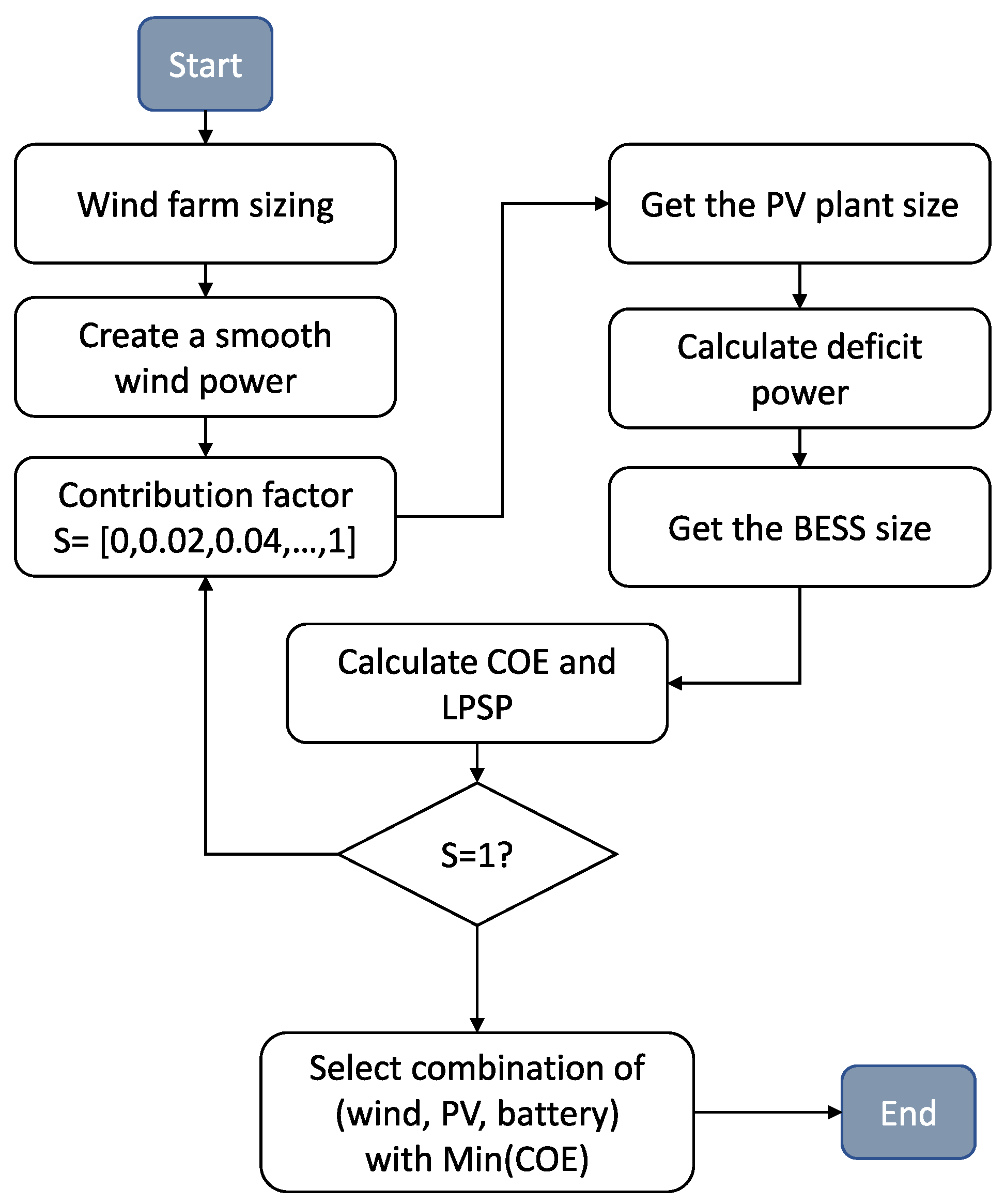
The integrated approach’s main goal is to size the HWSPS such that it is both cost-effective and dependable. The planned HWSPS is evaluated using cost of energy (COE) as a major performance indicator. The COE formula takes into account all of the components’ capital costs, operating and maintenance expenses, replacement cost, and salvage cost. The loss of the power supply probability (LPSP) is utilized for techno-economic assessment and comparison in this study. The LPSP is defined as the likelihood that the supply would be unable to meet demand, and its value varies from zero to one. The flow chart in
Figure 1 shows the phases of the suggested strategy for scaling the HWSPS. The procedure of defining the HWSPS capacity is divided into two major steps. In the first step, an ideal wind farm is determined using the evolutionary algorithm, subject to site dimensions and turbine spacing, while Jensen’s wake effect model is used to reduce power losses caused by wind turbines layouts. Based on the reference wind power obtained by the MAV, SG, Gaussian, and LWLR methods, a numerical iterative algorithm is used in the second stage to determine the best combination of PV plant and BESS in the determined search space.
3. Smoothing Techniques
To obtain a smoothed reference output power approximating the load demand, many smoothing techniques are utilized. An integrated approach has been developed, which uses moving average, locally weighted linear regression, Gaussian, and Savitzky–Golay techniques. The proposed strategy is different from previous studies in that it does not involve a load demand profile. The sizing approach was designed to utilize the selected site effectively for a grid-connected system. The focus of this research is to maximize the output power from a hybrid renewable power plant at a constant level based on the availability of renewable energy resources. It is assumed that the load demand variations are absorbed by the grid.
3.1. Moving Average
In this investigation, the moving average smoothing technique
is used to obtain a smoothed reference output power
, which represents the load demand. The
value is the reference for the optimal HWSPS plant. The smoothing wind window of MAV [
30,
31] must be manipulated carefully to reach the desired reference power. The mathematical interpretation of the k-period MAV is presented by Equation (
6):
3.2. Locally Weighted Linear Regression
Linear regression is a technique for determining the linear connections between input and output. For non-linear relationships between the input and the output, locally weighted linear regression (LWLR) [
32] is used. Unlike normal linear regression, LWLR does not use fixed parameters
; thus, it is a non-parametric algorithm used to smooth noisy signals. It is a memory-based method and uses training data that are local to the point of interest. The mathematical model of the LWLR is given by Equation (
7).
As with the moving average, specifying the span length is critical for the LWLR. The span is defined by the fraction (i.e., 0.057%) of the data points closest to the target point
. The data points within the span determine the smoothed value. The points outside the span have a zero weight. Thus, the smoothing process is local, since it uses only the local points in each span. Quadratic and linear models can be used in the regression. In this study, linear models are used. The tricube function [
33] is used to calculate the weights, as given by Equation (
8):
The fitted model is obtained for the target point , and the same process is repeated for all the data points. The mathematical representations and calculations for the LWLR are summarized in the following points:
- -
Define the span length;
- -
Obtain the regression weights for each data point in the span;
- -
Solve the LWLR problem to obtain
and
by taking the first derivative for minima, as shown in Equations (
9)–(
11):
- -
Finally, to obtain the corresponding -value for the target point , substitute in the line equation for and .
3.3. Gaussian Distribution
The Gaussian distribution is also known by other names, such as normal distribution. The Gaussian function is widely used as a smoothing operator for noisy data points. In addition, it is used in defining the probability distribution (histogram) of data. The Gaussian function follows the bell-shaped curve. It is a function of non-zero value and is symmetrical about the mean .
The probability distribution is described mathematically using the expression in Equation (
12) [
34]:
where
and
represent the mean and standard deviation, respectively. The term
is a constant that acts as a normalizer. The exponential term decays quickly as
t diverges from
. The rate of decay is influenced by the value of
. The curve of the Gaussian function is divided into three segments, defined as follows:
- -
Segment (I): ;
- -
Segment (II): ;
- -
Segment (III): .
These three segments combined have the highest probability value (99.72%), with respective weights of 68.26% (segment (I)), 27.18% (segment (II)), and 4.28% (segment (III)).
3.4. Savitzky–Golay
Instead of smoothing by averaging the data and making an aggressive change in the original signal, Savitzky–Golay [
35] is a simple smoothing algorithm that follows the pattern of the original signal. SG is performed by fitting a least square in each window. In general, it is a moving polynomial fit with constant weighting coefficients. These coefficients are called convolution integers. These sets of integers are selected based on the window size and the polynomial degree. A reference table for 25 window sizes is presented in [
36] and contains different values of convolution integers for quadratic polynomials. Alternatively, convolution integers could be defined based on approximation by polynomials. In our case, a window size of 31 points, i.e.,
with a quadratic polynomial ({ = 2) is used. Thus, the smoothed signal for a set of data points
with the length n is calculated using the formula in Equation (
13). The convolution integers are calculated using the Vandermonde matrix
as given by Equation (
14):
where
The power fluctuation
is measured at each smoothing technique’s time instant, taking the difference between the subsequent output powers, as shown in Equation (
15):
4. Case Study
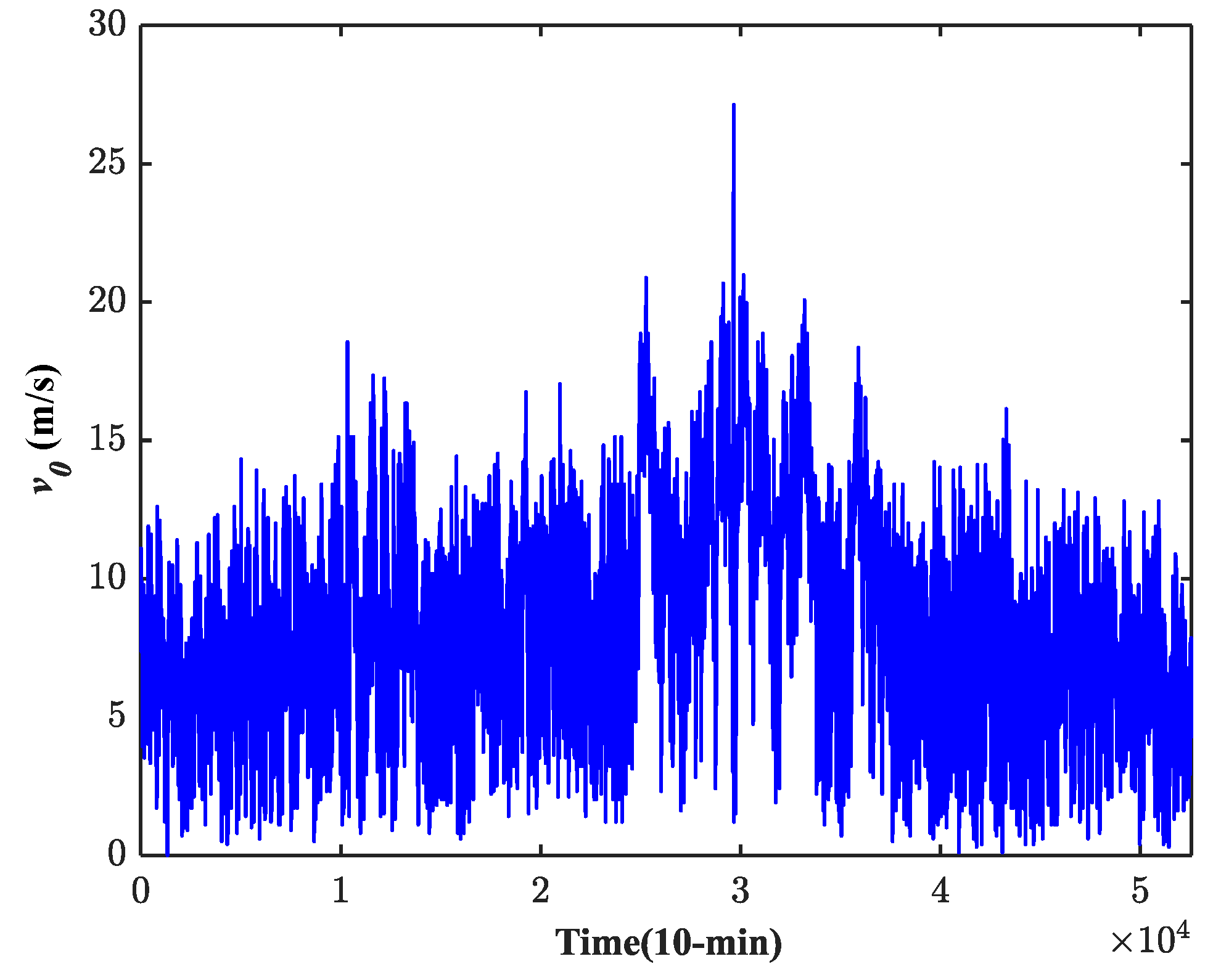
A case study has been provided to show the applicability of the suggested technique. The weather data from Thumrait, Dhofar Governorate, Oman, were utilized. This study makes use of wind speed and direction data collected throughout a year at a resolution of 10 min intervals. This histogram shown in
Figure 2 will be utilized in the optimization of the wind farm layout. After determining the farm size, the instant wind power
is calculated using real 10-minute wind profiles, whose wind magnitude is shown in
Figure 3. In addition, the PV output power is determined by utilizing the global horizontal irradiance of the mentioned site [
23].
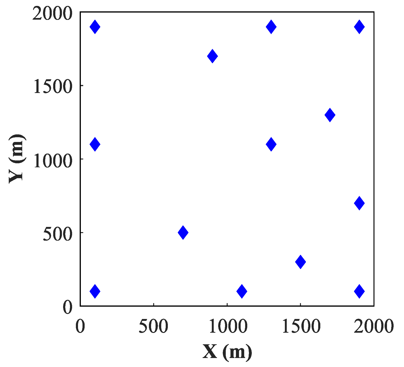
Table 1 lists the key technical and economic characteristics utilized in this analysis for the PV module, wind turbines, and BESS. For this study, a square land area is considered with dimensions of 2 × 2 km. The wind farm site is assumed flat with a surface roughness of 0.3 m.
5. Results and Discussion
Running the simulation with the data given produces results with 13 as the optimal number of turbines. They are distributed mainly along the WF’s boundaries to decrease the wake impact as shown in
Figure 4.
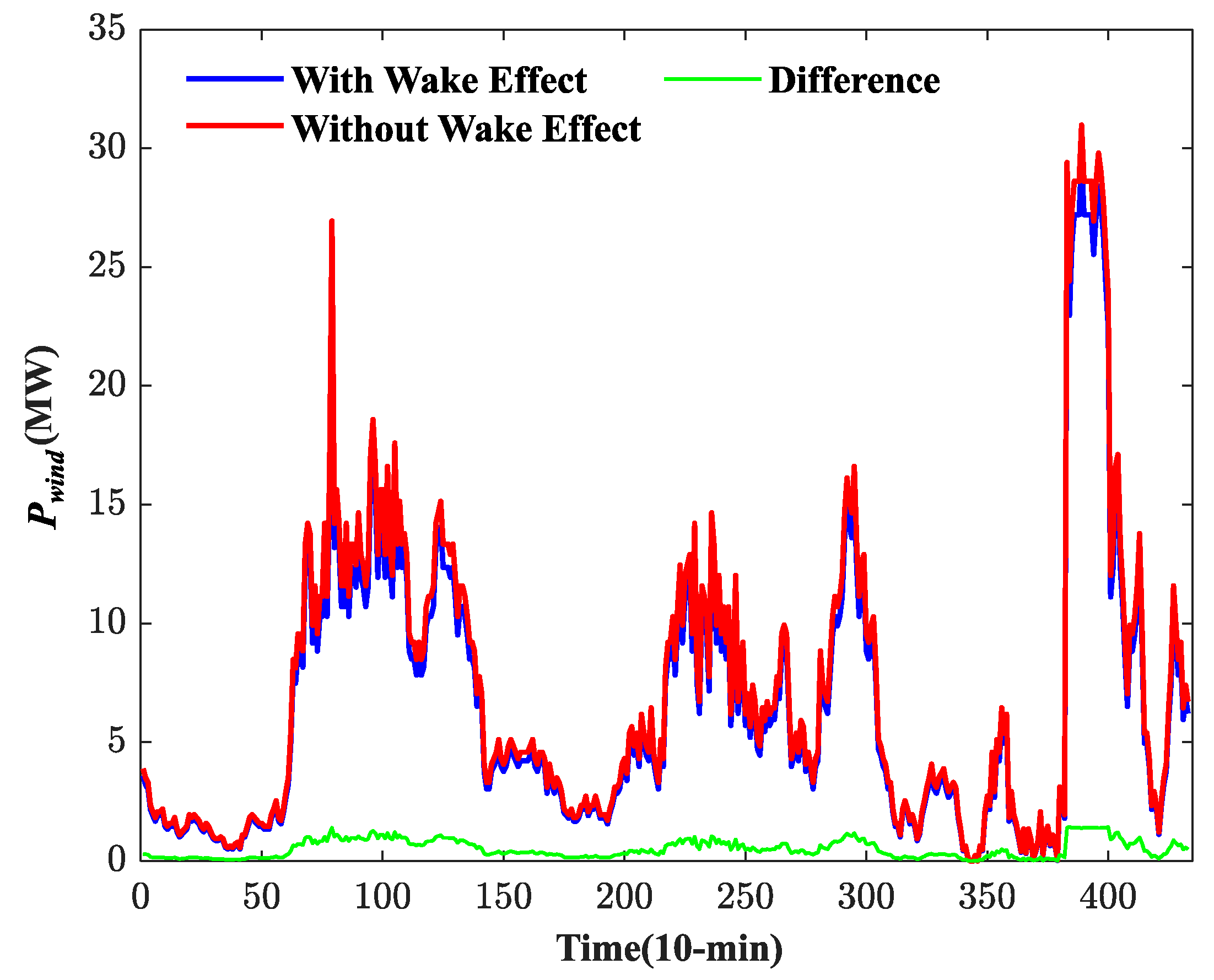
To demonstrate the wake effect’s impact on wind power generation in more detail,
Figure 5 depicts the power generation of the wind farm with and without the wake effect using the optimum configuration. The wake effect model produces more precise and realistic results for the power generation of a wind farm [
40]. The overall velocity loss owing to the turbine wake effect is approximately 2.72% of the available wind speed. This equates to a 5.31% decrease in the wind farm’s generating power. The distinction between the two situations is obvious, and utilizing the wake effect model enables planners to estimate more realistic wind farm power.
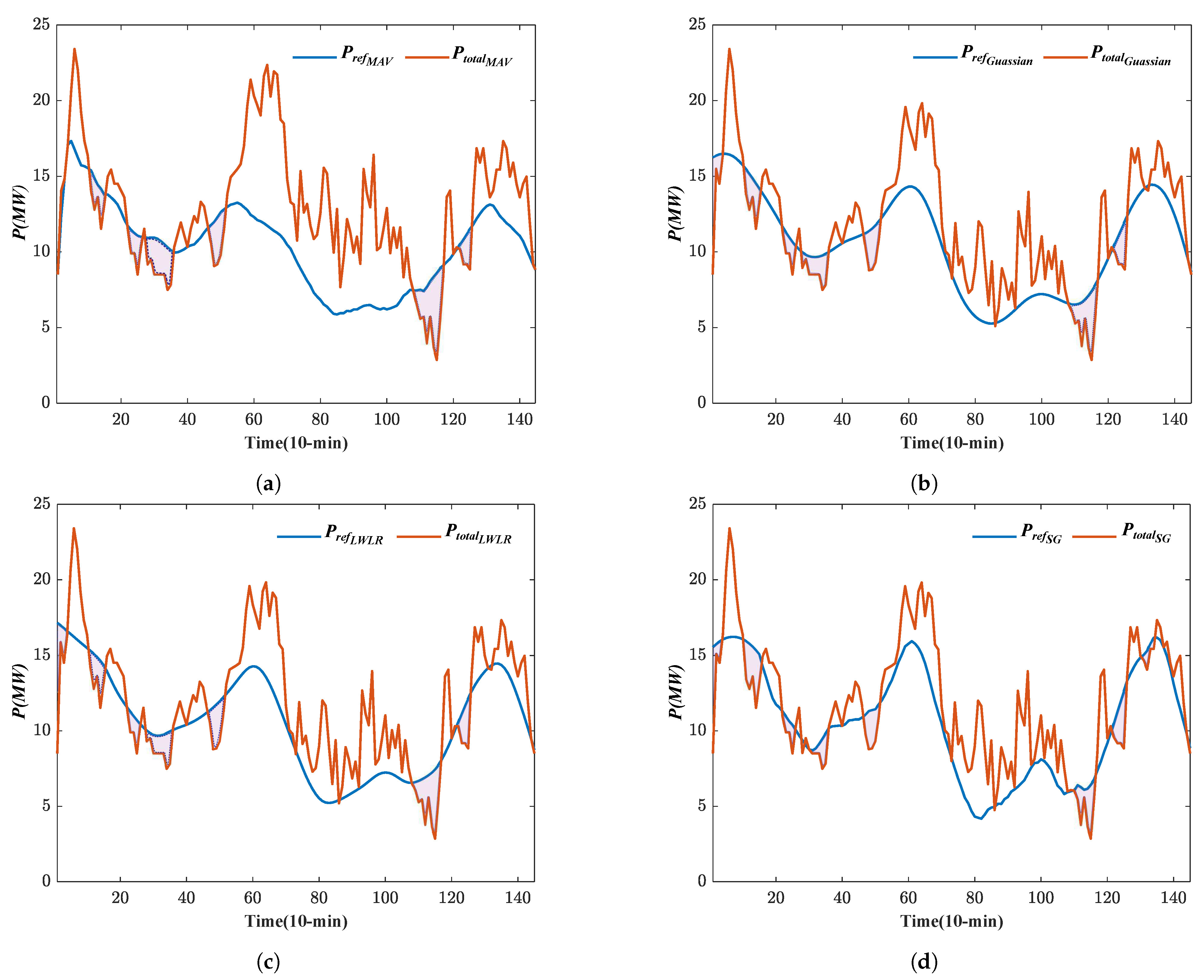
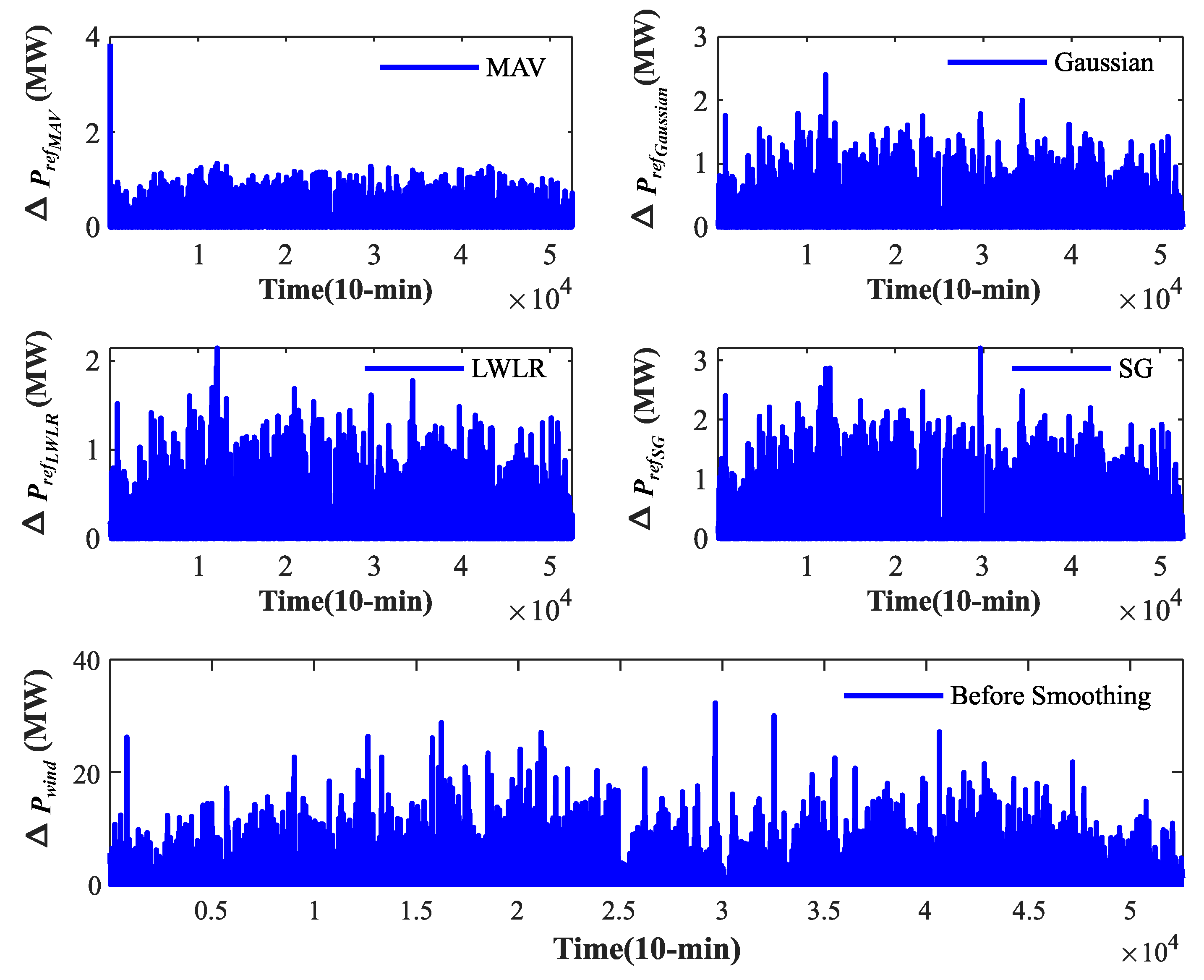
The suggested strategy then proceeds to create a smooth wind output power
utilizing the LWLR, MAV, Gaussian, and SG approaches to decrease variations in the wind farm’s output power with the help of a PV plant and BESS. The primary goal of smoothing wind generation is to minimize the ramping rate, as seen in
Figure 6. The ramping rates are displayed before and after smoothing. Before smoothing, the maximum ramping is 32.33 MW. After smoothing, the maximum ramping rates are 2.14 (with LWLR), 3.85 (with MAV), 2.40 (with Gaussian), and 3.20 MW (with SG). This means that the maximum ramping in
,
,
, and
correspond to 5.49%, 9.87%, 6.15%, and 8.21% of the wind farm’s capacity, respectively. These results are adequate to move on with this case study.
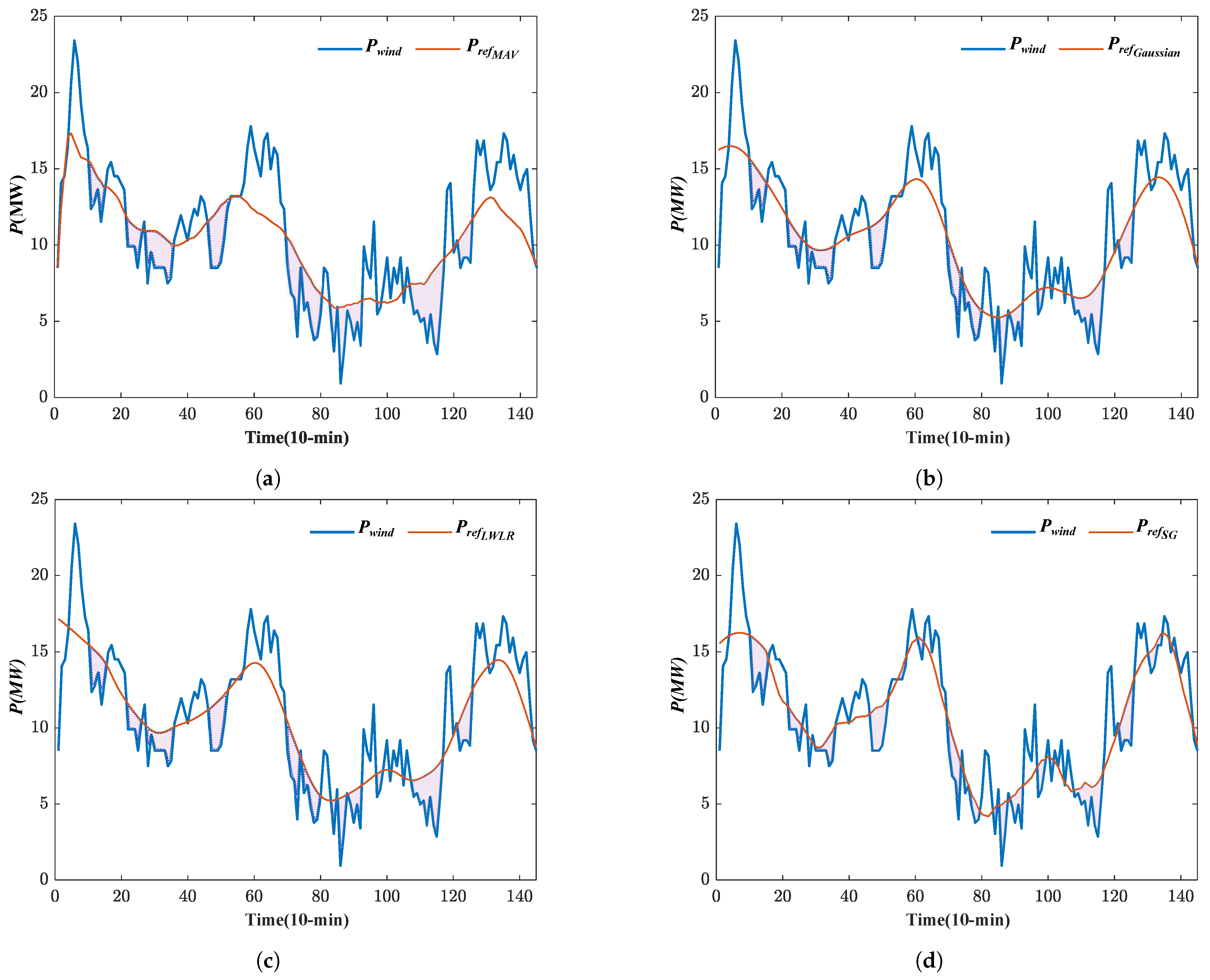
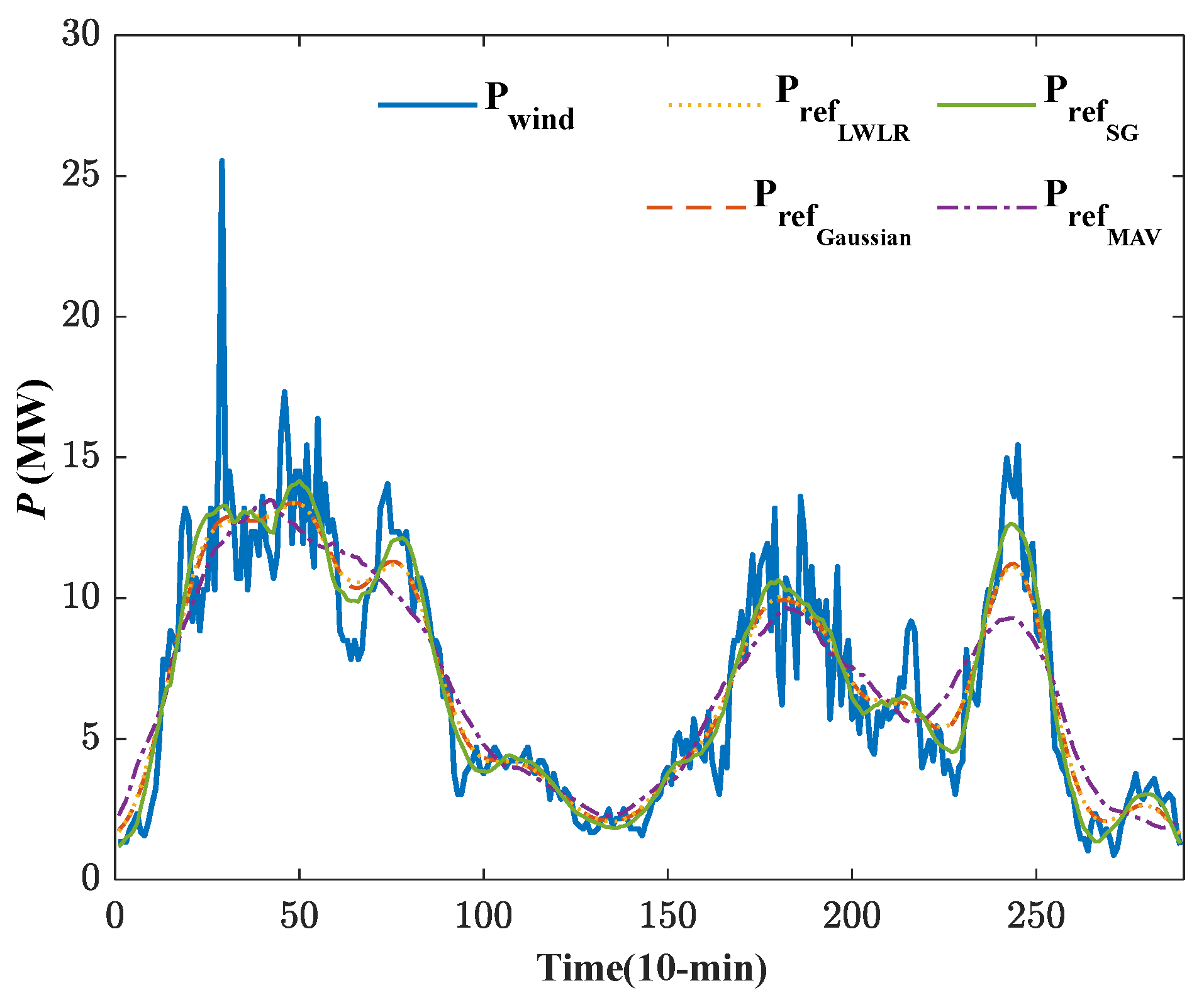
Each smoothing technique was used with 30 data points, and the generated
for each technique is shown in
Figure 7. It is obvious that
is smoother than
. The purple-bounded regions in
Figure 8 present how much
falls short of
. The gap between
and
is greater than that from other smoothing techniques. This means more resources are needed to compensate the generations. As a result, a PV plant and BESS with 50 contribution factors (S) were installed to alleviate the shortfall, as stated in
Section 2.
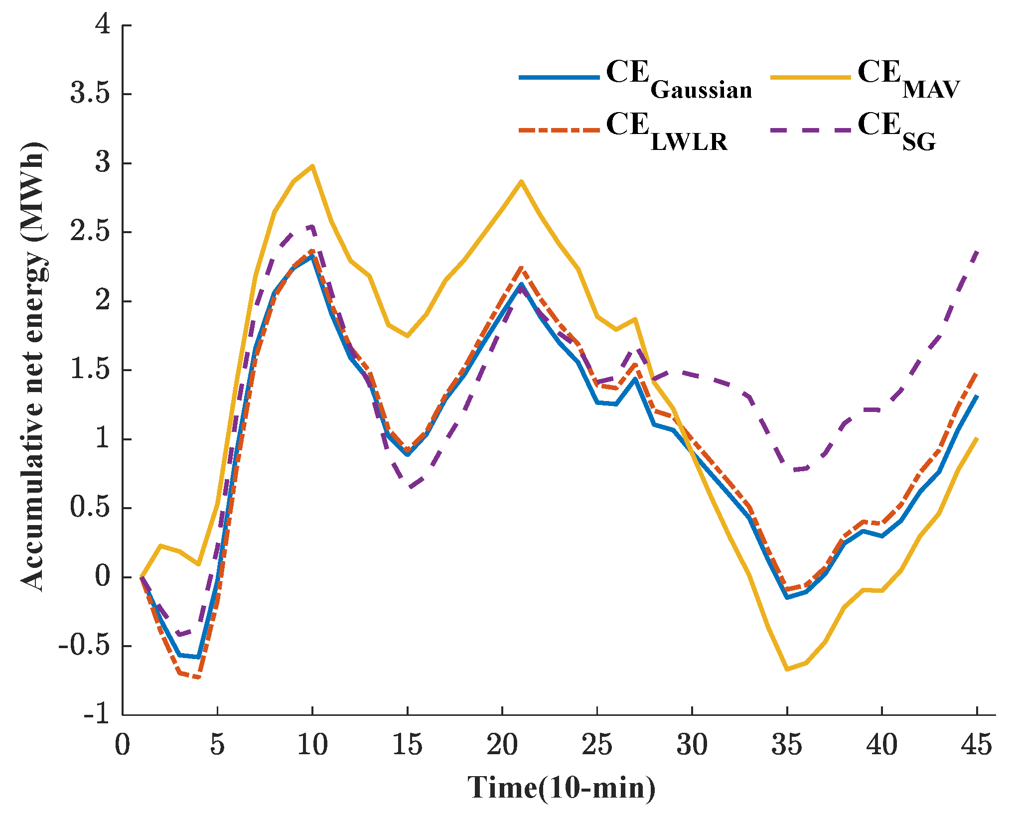
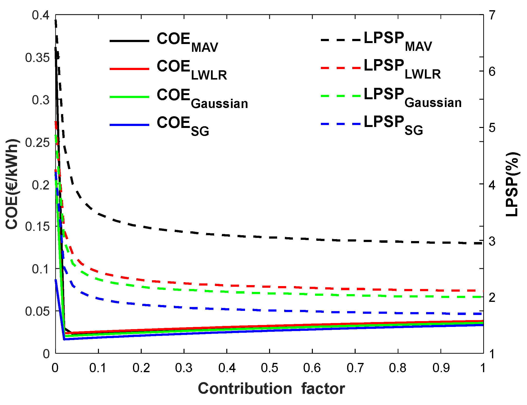
Running the suggested method in NIA produced several PV plant and BESS setups with COE and LPSP, as illustrated in
Figure 9. As the sizing of BESS is meant to minimize oversizing by considering just the minimal yearly negative accumulative net energy, the BESS size dropped with each increase in S for each smoothing approach, and finally the size was fixed. The minimum CE values for the whole year are 0.72609 (for LWLR), 0.6680 (for MAV), 0.57942 (for Gaussian), and 0.41753 MWh (for SG), as shown in
Figure 10.
The capacity of the BESS began at 18.74 MWh for S = 0, and then reached the minimum value of 0.8350 MWh for S = 0.04 (with the MAV). In addition, the minimum COE was 0.0229 EUR/kWh, with 10.716 MW for the PV plant sizes. The simulation results also attest to the effect of LWLR, Gaussian, and SG in smoothing the wind power to overcome the negative impact of the memory effect in MAV. Compared to MAV, the optimal sizes of the BESS and PV for LWLR, Gaussian, and SG were attained while S = 0.02. Thus, the optimal COE was 0.0237 EUR/kWh (for LWLR), 0.0203 EUR/kWh (for Gaussian), and 0.0165 EUR/kWh (for SG). However, the COE for LWLR was the highest, due to the size of the BESS, which reached 0.9076 MWh.
On the other hand, the BESS for the SG was 0.2024 MWh lower than the BESS size for the Gaussian. The PV size was 5.329 (for LWLR), 5.329 (for Gaussian), and 5.305 MW (for SG). These techniques yielded similar PV size values, in contrast with MAV, which yielded a value of 10.716 MW.
Table 2 shows an overview of the best outcomes.
As shown in
Figure 11, the values still fall short of the reference power, but the whole LPSP values for the entire year are 4% for MAV, 3.17% for LWLR, 2.99% for Gaussian, and 2.52% for SG. The largest loss comes at night when PV generation is not available. The size of the PV plant grows linearly as the contribution factor S increases, resulting in larger fluctuations and more damped output.
With an increase in a contribution factor, the power deficit reduces, but the COE rises. Simultaneously, the BESS SOC varies substantially between and . (charged and discharged condition). During the day, there is enough to compensate for the wind generation shortfall. A portion of the surplus energy is used to power the BESS. Due to the tiny size of the PV plant, the BESS is usually employed if the LWLR, Gaussian, or SG are used. The BESS is the most commonly used with LWLR, followed by Gaussian and then SG. Due to the huge size of the PV plant, the MAV uses the BESS the least. MAV, on the other hand, has a greater COE and a lower LPSP than SG.
6. Sizing without the Wake Effect
A simulation was run to determine the best HWSPS without taking into account the wake effect. For each smoothing approach, the simulation was run using the optimum contribution factor. With the MAV set to S = 0.04, this resulted in a HWSPS with a PV plant of 11.372 MW and a BESS of 0.8984 MWh. The PV plant and BESS sizes rose by 6.12% and 7.59%, respectively. The optimum PV and BESS sizes for the SG for S = 0.02 were 5.63 MW and 0.5319 MWh, respectively. Running the simulation with S = 0.02 and the Gaussian model resulted in a HWSPS with a 5.66 MW PV plant and a 0.7418 MWh BESS. Finally, when compared to the wake findings, the sizes of PV and BESS rose by 6.12% and 2.91%, respectively, using the LWLR method. This illustrates the overestimation that happens when estimating the HWSPS size without taking the wake effect into account.
7. The Influence of Contribution Factor on PV Plant and BESS Sizes
The wind farm’s cost alone is less than the optimal cost of the proposed HWPS. However, the LPSP of a HWSPS with MAV is 4%, compared to 6.91% for a stand-alone wind farm, implying that the HWSPS is roughly 2.91% more reliable. These findings demonstrate that a wind farm alone is not a dependable solution.
Increasing the size of the PV plant and the BESS improves the LPSP but raises the COE. Furthermore, the surplus electricity grows, resulting in a decrease in revenue. Thus, the availability of other resources on a wind farm benefits the electrical system, but only up to a certain degree of resource penetration.
8. Summary
In this paper, an approach was developed to mitigate the wind output power fluctuation. It focuses on scaling the HWSPS to decrease the impact of renewable energy resource intermittency and provide maximum output power to the grid at a consistent level on a timely manner based on renewable energy resource availability. The PV and BESS are sized dependent on the production of the wind farm. Unlike earlier research, this technique does not consider the load profile when sizing the HWSPS. The appropriate size of the HWSPS is determined using the smoothed wind power signal as a reference. The smoothed signal is generated using the MAV, LWLR, SG, and Gaussian smoothing techniques.
Furthermore, the GA is employed in the initial step of the method, with Jensen’s wake effect model being applied to provide more precise and realistic results. The research focuses on sizing the HWSPS in order to decrease production variations and enhance dependability of the wind farm. The NIA is used to size the PV plant and the BESS, which is a trade-off between system cost and reliability.
The suggested method was shown using real GHI data from a wind power plant site in Oman with a multi-speed and multi-directional wind profile. The wake impact on turbines was shown, and the power outputs of the wind farm with and without the wake effect model were compared. The optimal HWSPS had a wind to PV ratio of 3.64:1 with MAV and around 7.32:1 with other smoothing techniques. The corresponding BESS capacity represented 1.68% of the HWSPS’s rating for MAV, 2.05% for LWLR, 1.18% for SG, and 1.63% for Gaussian.
The results also show that the SG smoothing technique is more suitable for this task than MAV, Gaussian, or LWLR techniques. It was also found that the window size plays a vital role in the smoothing of noisy output, but this smoothness has a negative impact on the cost of energy. The memory effect feature of the presented smoothing techniques led to a delay between the smoothed signal and the actual signal. In general, this implies an increase in the smoothing source capacities.
In addition, an evaluation of the influence of the wake effect and the contribution factor on the sizing of the HWSPS was conducted. This evaluation revealed the importance of the wake effect to avoid overestimating the HWSPS size. As a result, the suggested method is efficient in conducting a feasibility study for the size of a HWSPS in order to achieve a cost-effective and dependable system.


