Article

Mobile GPS Application Design Based on System-Level Power and Battery Status Estimation †

1
Department of Electronic Engineering, Myongji University, Yongin 17058, Korea
2
School of Electrical Engineering, Korea Advanced Institute of Science and Engineering (KAIST), Daejeon 34141, Korea
3
Department of Smart Systems Software, Soongsil University, Seoul 06978, Korea
*
Author to whom correspondence should be addressed.
This paper was presented in part at the 2013 Asia South Pacific Design Automation Conference (ASP–DAC), Yokohama, Japan, 22–25 January 2013.
Energies 2021, 14(17), 5333; https://doi.org/10.3390/en14175333
Submission received: 28 July 2021 / Revised: 16 August 2021 / Accepted: 23 August 2021 / Published: 27 August 2021
(This article belongs to the Special Issue Thermal and Energy Management of Battery-Operated Systems)

Abstract

:
Mobile systems such as smartphones require accurate estimation of the battery-related features including the remaining energy and operating time, especially as the the power consumption of user applications is growing continuously these days. We present an energy-aware smartphone application design framework that considers the battery’s state of charge (SOC), energy depletion rate, as well as the service quality of the target application. We use a verified-accurate battery energy estimation method in an Android-OS-based mobile computing system. The battery model considers the rate-capacity effect. We apply regression-based models for the power estimation of the major subsystems in the smartphone, and then aggregate the result to yield the whole system’s power. We first determine the quality of service for the location device (GPS), the display device (LCD), and the overall system (application). Then, we control the error rate of the GPS and the brightness of the display to acquire the maximum service quality of the system for a given car trip. We show the advantage of the proposed method with a case study of a trip. In this case, the smartphone guides a user’s car trip using its GPS navigation capabilities; to do this, we propose an adaptive algorithm that exploits our improved SOC estimation and considers the car’s variable velocity. This proposed adaptive power and service quality control of the GPS application improves the quality of service in this example case and ensures there is enough remaining battery for the trip to be completed. In contrast, conventional approaches to this task provide a lower quality of service and run out of battery before the trip finishes. In conclusion, if a trip plan is provided, an application using our method delivers the maximum quality of service, such as system endurance time, location error, and display brightness.

1. Introduction

Modern high-performance mobile computing systems are increasingly consuming more power. These applications simultaneously support various functionalities, including the display, audio, GPS, wireless communication, and higher computing capability with only limited energy stored in the batteries. However, the increases in the energy density of batteries has been much slower, and it merely satisfies the expectations of the users. As a result, it has become critical to utilize the precious energy stored in these batteries. Accurate power modeling and estimation is the starting point of power and energy management.
Extensive studies have been conducted on the power analysis and modeling of mobile embedded systems. Among the models, parameterized power models based on the system parameters are considered a convenient approach to use in a run-time manner. A measurement-based power estimation model was introduced in [1], where the system activity parameters were collected and evaluated from the viewpoint of the system power consumption. These coefficients of the system power equation were derived by regression analysis.
There have been several efforts to provide system-level power estimation models for smartphone platforms [1], including some battery-information-based models [2,3]. These models are based on the component activities within the system. For accurate online estimation of the battery SOC, combining particle swarm optimization and extended Kalman filter [4], co-estimating load current and SOC without a physical sensor [5], and diagnosing of internal short circuit of the battery [6] have been intensively studied. The dependencies between the system energy models on hardware architectures and configurations were studied in [2]. The possible usage patterns were analyzed at the same time to suggest personalized models for battery-powered mobile systems. An on-chip bus performance monitoring unit was introduced to generate the system power consumption model in [7]. A run-time, feedback-based, full-system energy estimation model for battery powered devices was introduced [8]. A power consumption model for wireless applications with OS-level parameters was constructed [9].
In practice, commercial smartphones are usually equipped with built-in battery voltage sensors. Then, it utilize previously explained battery discharge behavior models to calculates the lifetime. It is a straightforward method that has been introduced for earlier smartphones [3]. It was claimed that the proposed method achieves accurate enough result up to commercial level. An improved method considering the rate capacity effect and battery internal loss was introduced [10].
We introduce an energy-aware application design framework for Android-OS-based mobile systems considering the practical aspects of battery behavior. As a case study, we explored the design through a GPS application from the perspective of service quality and service time based on a battery capacity loss estimator and power consumption model using the Android kernel, which produced accurate subsystem activity data in our prior work [10]. As a trade-off exists between battery lifetime and service quality of the GPS application considering the locating resolution and trip coverage [11,12]. A trade-off between the locating resolution and power consumption was considered when designing the sensor node application in [13,14]. In [15,16,17], a sensor-GPS hybrid location technique was studied. It also an intensively studied topic for electric- or GPS-based autonomous vehicles [18,19].
We consider the other major power consumers in these mobile systems, including the display. We finally construct an adaptive algorithm to maximize the battery lifetime by adjusting the GPS location precision and display brightness according to velocity variations during the trip. The remainder of this paper is organized as follows: We introduce the structure of the proposed method in Section 2. Then, we show that the proposed adaptive power and service quality control of the GPS improves the quality of service in Section 3. We present the formulated service quality optimization problem and its solution method in Section 4. The experimental results are provided in Section 5, and the conclusions in Section 6. Note that the detailed power estimation model on the Odroid-A platform is introduced in Appendix A and Appendix B.

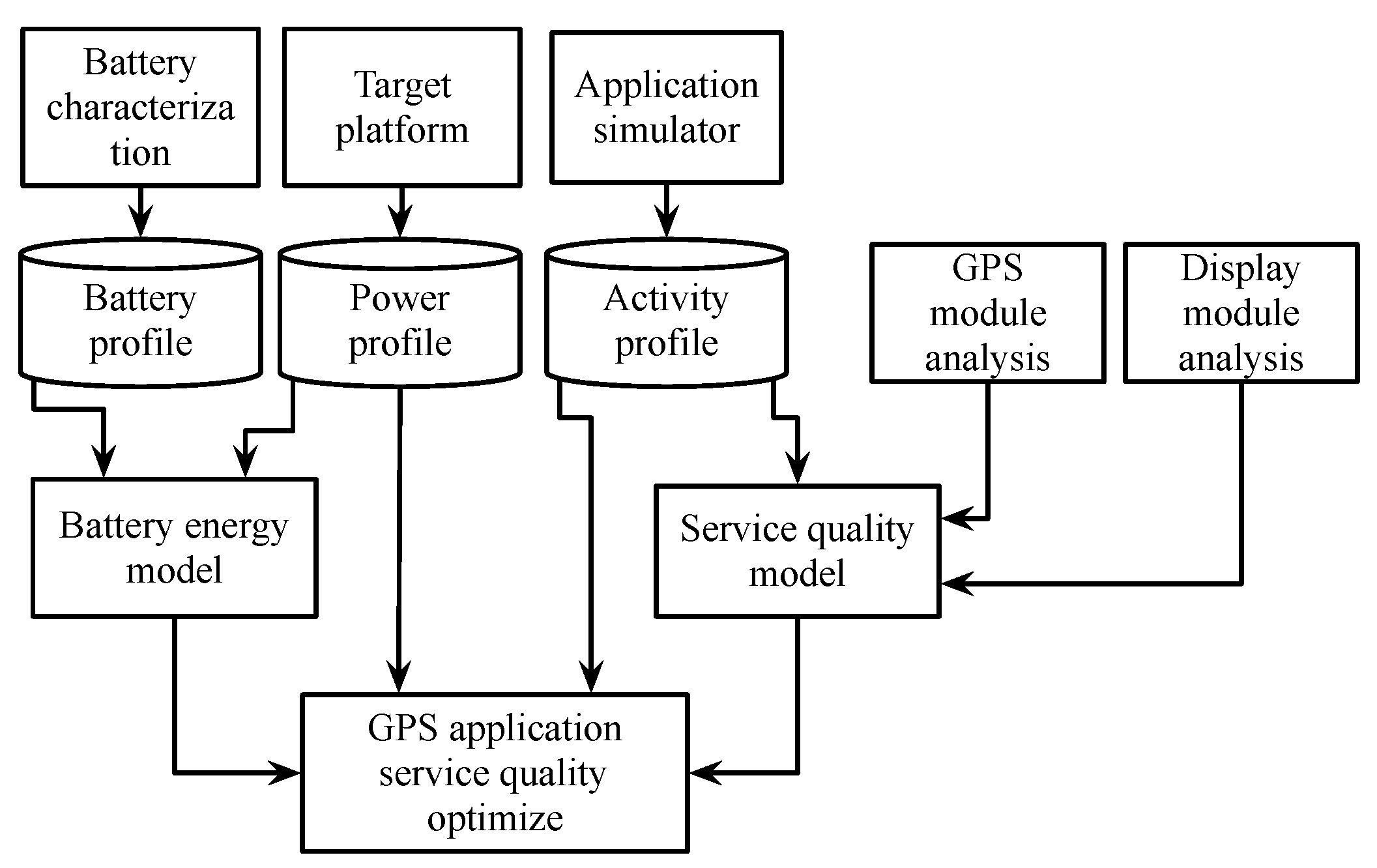
2. Energy-Aware Application Design Framework

Figure 1 shows the proposed application design framework to optimize the service quality of GPS applications. In the framework, the system power consumption and the battery SOC of the target platform are estimated using the system and battery models constructed in our previous work [10]. The models are described in Appendix A and Appendix B. We characterized the internal battery by measurement as we charged and discharged the battery in constant-current and pulse-current situations. We also considered a rate-capacity effect for accurate modeling. We present the modeled battery parameters in Appendix A. We also performed a regression analysis for the power consumption of each component of the target smartphone and extract the coefficient of the power model. The components of the target smartphone and their coefficients are described in Appendix B. We built a service quality model of the GPS application to maximize the satisfaction of the smartphone user. Since higher performance requires more power, if we set a smartphone in high-performance mode, its battery depletes faster. However, a typical user prefers to have a running smartphone with reduced performance rather than one that is completely turned off. Thus, it may be better to limit performance to make smartphones last last in certain cases. We regard the locating accuracy and display image quality as the performance of the GPS application. The GPS module has a trade-off relationship between its locating accuracy and power consumption. Like the GPS module, the brightness (and thus the dynamic range) of the display device is also proportional to the power consumption in general [20]. We therefore designed the GPS application to balance locating accuracy, display image quality, and service time with the objective of maximizing the service quality.

3. Adaptive Control of Service Quality and Power Consumption

Mobile devices should remain turned on until they are connected to wall power. sSometimes, they cannot remain on because the energy capacity of mobile devices’ batteries is limited. Limiting the performance of mobile devices can save the remaining energy of the batteries. In general, it could be beneficial to limit the performance of the device to prolong operation time since users prefer using mobile devices with limited performance rather than being unable to use them. We suggest an energy-aware application that limits the performance of GPS and reddisplays to make mobile devices work longer.

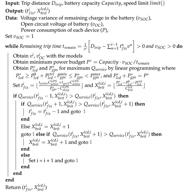
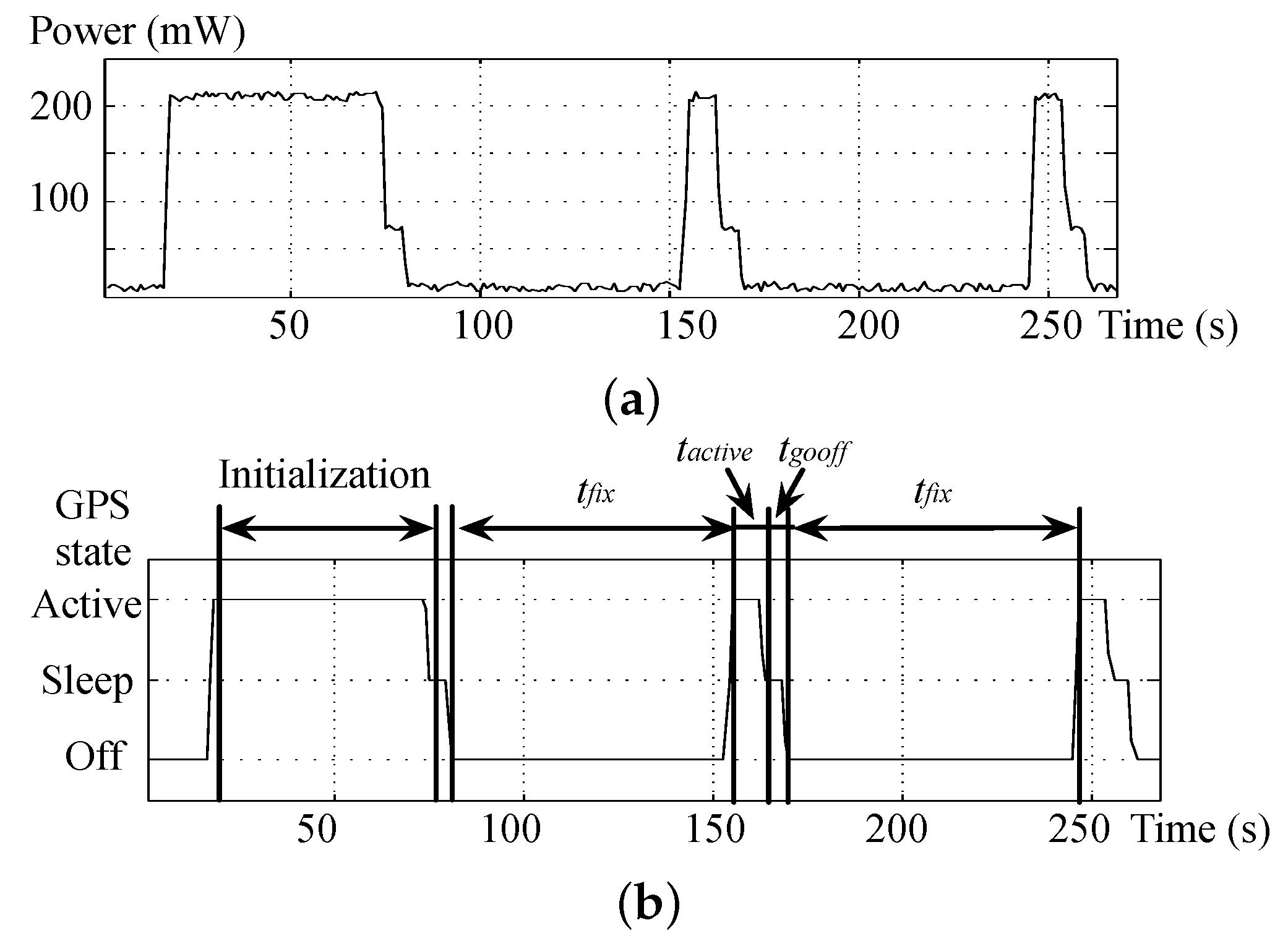
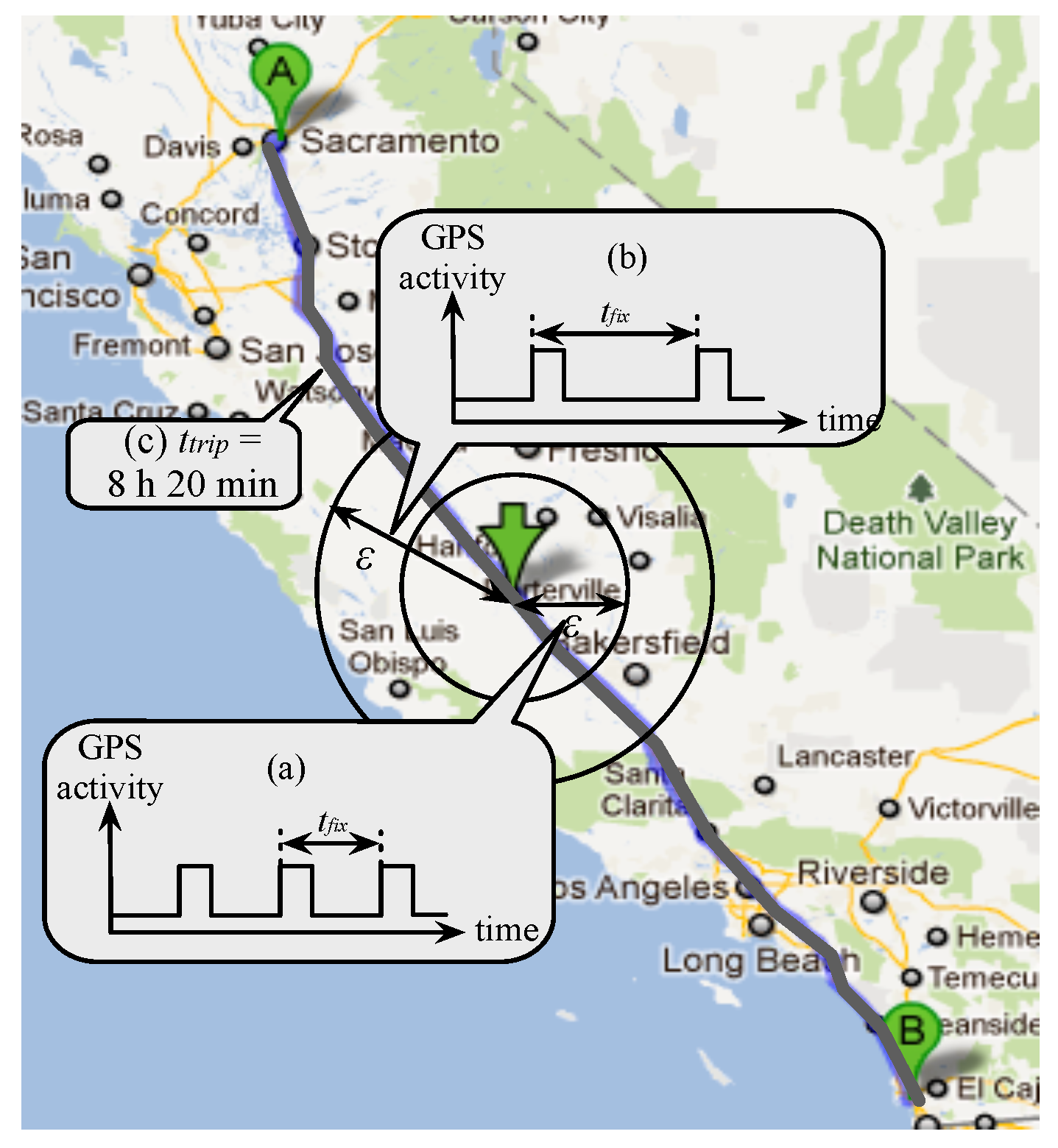
3.1. Service Quality of GPS Module

When its host system has a limited energy budget, a GPS application should have lower power consumption remaining enough accuracy. Note that in this paper, lifetime denotes a duration lasting until the system is turned off because of battery depletion. Under certain circumstances, lifetime is more important than locating accuracy. For example, if a user is in an emergency in a strange area, a longer service time is required. If a user travels on a long-distance trip, the required accuracy may be less. Note that the locating accuracy may be critical such in systems such as aeronautical navigation systems, but we do not target that system here. We evaluated the the service quality of a GPS application considering both the locating accuracy and service time. Table 1 explains the symbols used in this work. Faster GPS tracking of an object increases the error. S longer fixing period of the GPS also results in increased error. We model the maximum locating error of the GPS [10] as:
ϵ = v · t f i x + ϵ 0
where v, t f i x , and ϵ 0 are the velocity of tracking object, th fixing period of the GPS, and the fundamental GPS error, respectively. Figure 2a,b shows that tshe longer t f i x has larger error per Equation (1). We normalized the error when we evaluated the service quality error of th GPS application. We also considered service time when we evaluated the quality of service. If the installed battery of the mobile device is not depleted until a given trip is finished, the normalized trip coverage ( C o v e r a g e ) is the maximum. We set the maximum value of C o v e r a g e to 1, and we set C o v e r a g e proportional to the covered trip time if the internal battery is depleted before the trip is complete; thus, we formulate the normalized trip coverage as:
C o v e r a g e = t s e r v i c e / t t r i p ( t s e r v i c e t t r i p ) , 1 ( otherwise ) ,
where t s e r v i c e and t t r i p are the service time and the given trip time, respectively. We calculate the energy used when the GPS application is running from Equations (A4) and (A5). We denote the power consumption of the other devices as E o t h e r ¯ . The used energy is estimated as:
Δ E G P S ¯ = Δ t ( C o f f G P S X o f f G P S ¯ + C s l e e p G P S X s l e e p G P S ¯ + C a c t i v e G P S X a c t i v e G P S ¯ ) + Δ E o t h e r ¯ + E l o s s ,
The Android API requestLocationUpdate() supports various fixing periods of the GPS. We analyze power consumption and duration depending on the state of the GPS, as shown in Figure 3. We model the state duration ratio proportional to t t o t a l as:
t t o t a l = t f i x + t a c t i v e + t g o o f f , X a c t i v e G P S ¯ = t a c t i v e / t t o t a l , X s l e e p G P S ¯ = t g o o f f / t t o t a l , X o f f G P S ¯ = 1 X a c t i v e G P S ¯ X s l e e p G P S ¯ .
We assume that t f i x is always longer than t g o o f f or t a c t i v e . t a c t i v e and t g o s l e e p are the time duration of the ACTIVE state and SLEEP state, respectively. The t s e r v i c e in Equation (2) is obtained by dividing the battery capacity by Δ E G P S .

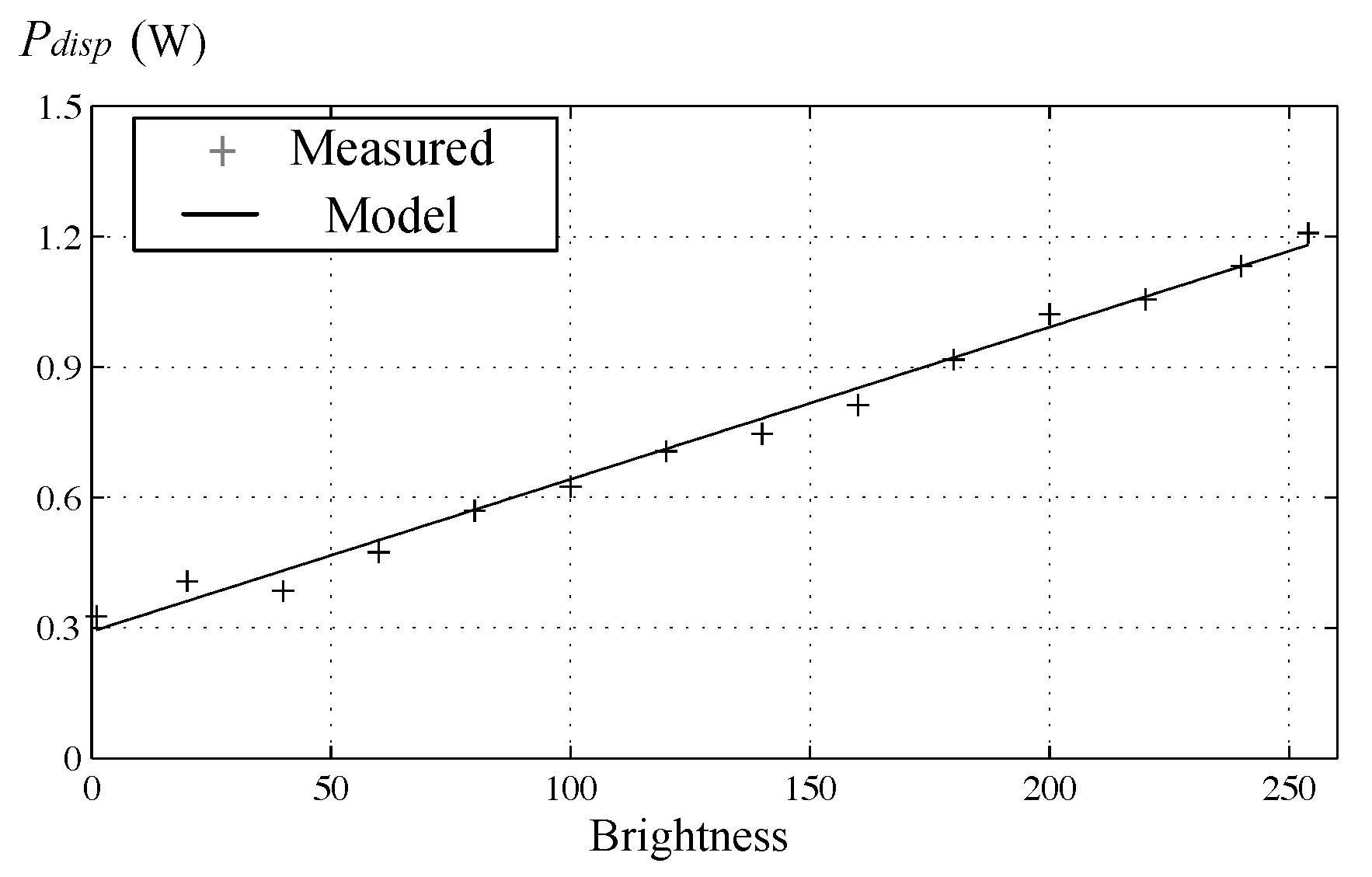
3.2. Display Image Quality

Display devices are some of the major power consumers in mobile electronics. An LCD is not a self-illuminating device; therefore, the light intensity is determined by the backlight intensity and its transmissive efficiency. The backlights of LCDs have been implemented with CCFL or LED. Nowadays, LED backlights are more popular due to their low power consumption, long lifetime, and excellent stability.
The light intensity from an LED backlight is basically proportional to the current that flows through the device, where the number of emitted photons per time is the same as the number of charges per time, in other words, the current. The LED has an internal resistance and a threshold voltage in the equivalent circuit model. We need to supply enough voltage to flow the required current to illuminate the device as we want. Therefore, theoretically, the power consumption of the backlight is proportional to the square of the maximum required light intensity.
However, the LCD consumes power linearly proportional to brightness because the relationship between physical light intensity and human-perceived brightness is nonlinear. Thus, the brightness value of the image data is tuned by a gamma table. The power consumption becomes proportional to the brightness after the gamma tuning is applied, as shown in Figure 4. This figure shows the measured power consumption and the plot produced by the model when we change the brightness parameter in the Android OS.
The maximum brightness determines the dynamic range of the display, which is directly related to the displayed image quality. We normalize the displayed image quality using the maximum brightness by:
Q l c d = X b r i t l c d m a x ( X b r i t l c d )
where m a x ( X b r i t l c d ) is the maximum brightness.

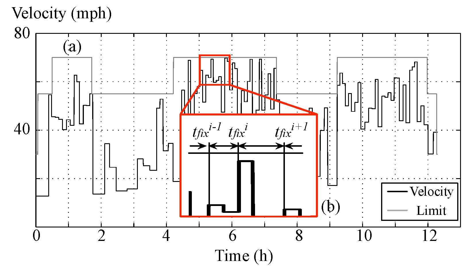
3.3. Adaptive Energy-Aware Service Quality Control

In practice, the velocity of a vehicle changes over time. Figure 5a shows the speed limit along the route from San Diego to Sacramento. Different speed limits are applied in residential areas urban freeways, and rural freeways. We assume that the velocity changes randomly within the speed limit. We model the trip in a discrete manner using t f i x intervals. The next fixing time interval, t f i x i + 1 , is determined at each fixing time, as shown in Figure 5b.
We define the combined service quality Q s e r v i c e as a weighted sum of the GPS trip coverage, GPS location error, and displayed image quality, which is given by:
Q s e r v i c e = ω 1 · C o v e r a g e + ω 2 · 1 ϵ + ω 3 · Q l c d
where ω 1 , 2 , 3 represent the weight values, and the definition of each service quality metric is presented in Section 3 and Section 3.2.

4. Problem Formulation

We maximize the service quality for the given trip time, power model, and battery model. The problem statement is as follows:
Problem 1.
Determine ( t f i x i , X b r i t l c d , i ) to maximize Q s e r v i c e for a given trip time, power model, and battery model.
This problem can be regarded as an integer programming problem where ( t f i x i , X b r i t l c d , i ) is regarded as a tuple of discrete values. If the velocity profile is given in advance, we can find the global sub-optimum by using a branch-and-bound algorithm or integer-linear programming. Otherwise, we should make a decision considering service time as well as the service quality in a heuristic way. The decisions made at each epoch are dependent on each other through a nonlinear dependency among the battery internal resistance R t o t a l , battery output voltage v O C , and battery SOC. The current battery status and energy consumption are dependent on the previous decision.
We propose the heuristic algorithm presented in Algorithm 1 based on a relaxed solution in a continuous domain with iterative hill climbing. The location determines the velocity at any given point during the trip. We assume that the driver obeys the speed limit, then the velocity at the ith decision epoch varies with the upper and lower speed limit. The SOC of the battery is also discretely calculated using Equations (A3)–(A5), where Δ t is determined by t f i x i .
Algorithm 1: Adaptive service quality and power control algorithm with variable velocity.
Energies 14 05333 i001

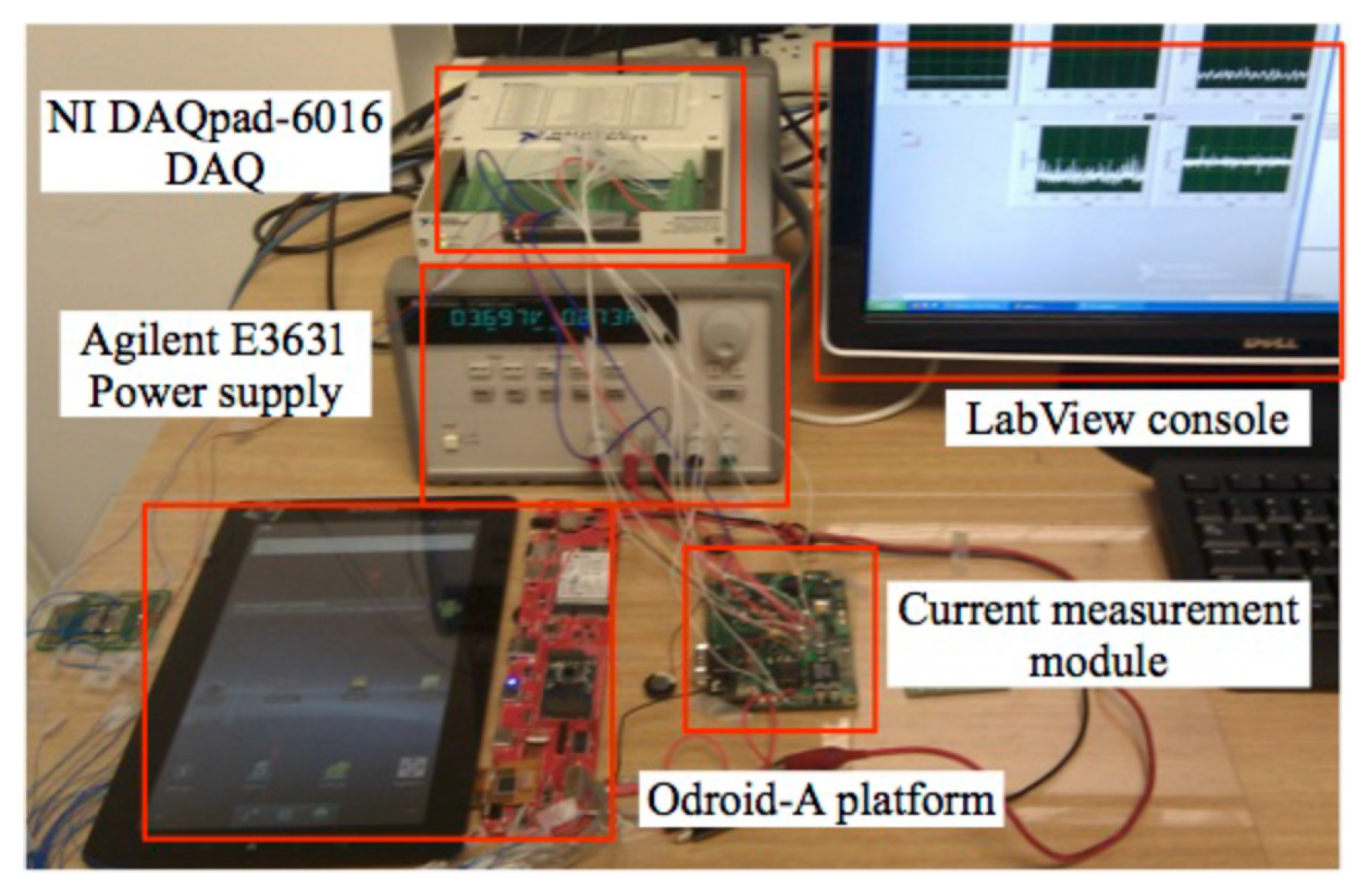
5. Experimental Methods

We set up an environment to extract the coefficients for the system power consumption model with Hardkernel’s [21] Odroid-A platform. We measured the current of the Odroid-A platform using shunt resistors and Texas Instrument’s INA194 [22] current sense amplifier. We collected the measured current data with National Instrument’s [23] DAQPad-6016 and LabView. Agilent’s E3631 [24] provided the power of the Odroid-A platform and the current measurement module. We double-checked the measurement data using a digital multimeter. Figure 6 shows the experiment setup. We present the battery and target system power model in Appendix A and Appendix B. All the coefficients extracted from the experiments are listed in Table A3.

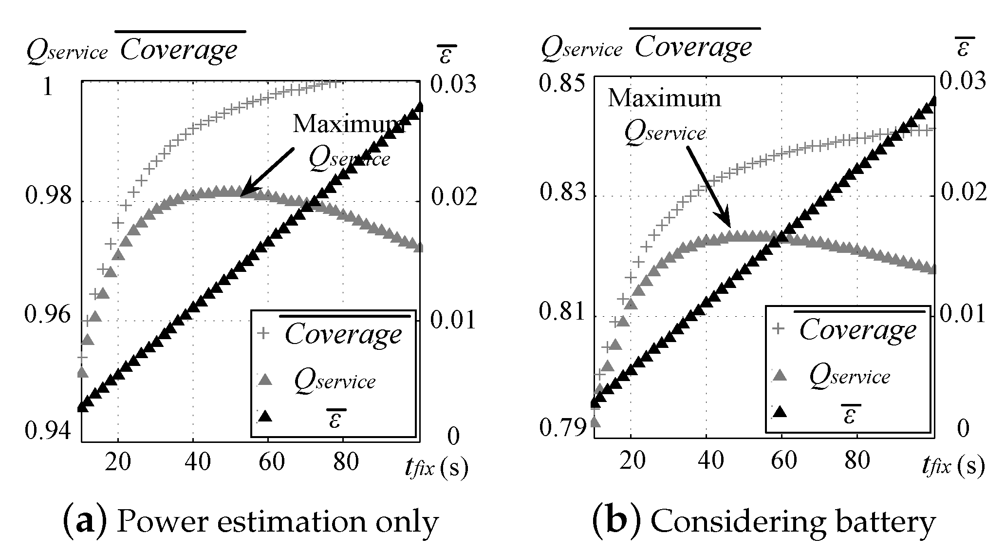
5.1. Accurate Energy Budget Considering Battery Internal Loss

We first show why we should consider battery internal loss for power-related calculations of mobile devices using an example case shown in Figure 2c. We assume that we travel the 523 mile road from Sacramento to San Diego with a fixed velocity of 60 mph. The estimated trip time is 8 h and 20 min when we check with Google maps. The battery and target system model used in this calculation are presented in Appendix A and Appendix B. In this example comparison, we simplify the energy consumption other than GPS as 3.5231 J. We also assume that t a c t i v e and t g o o f f are 10 and 5 s, respectively. We depict that the GPS application’s quality of service Q s e r v i c e depends on t f i x . C o v e r a g e ¯ and ( 1 ϵ ¯ ) are the estimated normalized trip coverage and the normalized accuracy, respectively. Figure 2a shows a higher Q s e r v i c e than Figure 2b, but it is unrealistic since there is no mobile device that does not use a battery. In other words, if the battery internal loss is not taken into account, the wrong power budget is expected, which makes the mobile device’s usage time prediction wrong as shown in Figure 7. For example, if we set t f i x to 80 without considering the internal battery loss, it seems that the mobile device can run until the trip is finished as shown in Figure 7a. However, this is not true. If we consider the realistic conditions, Figure 7b shows that the battery depletion forces the mobile device off when t f i x is 80.

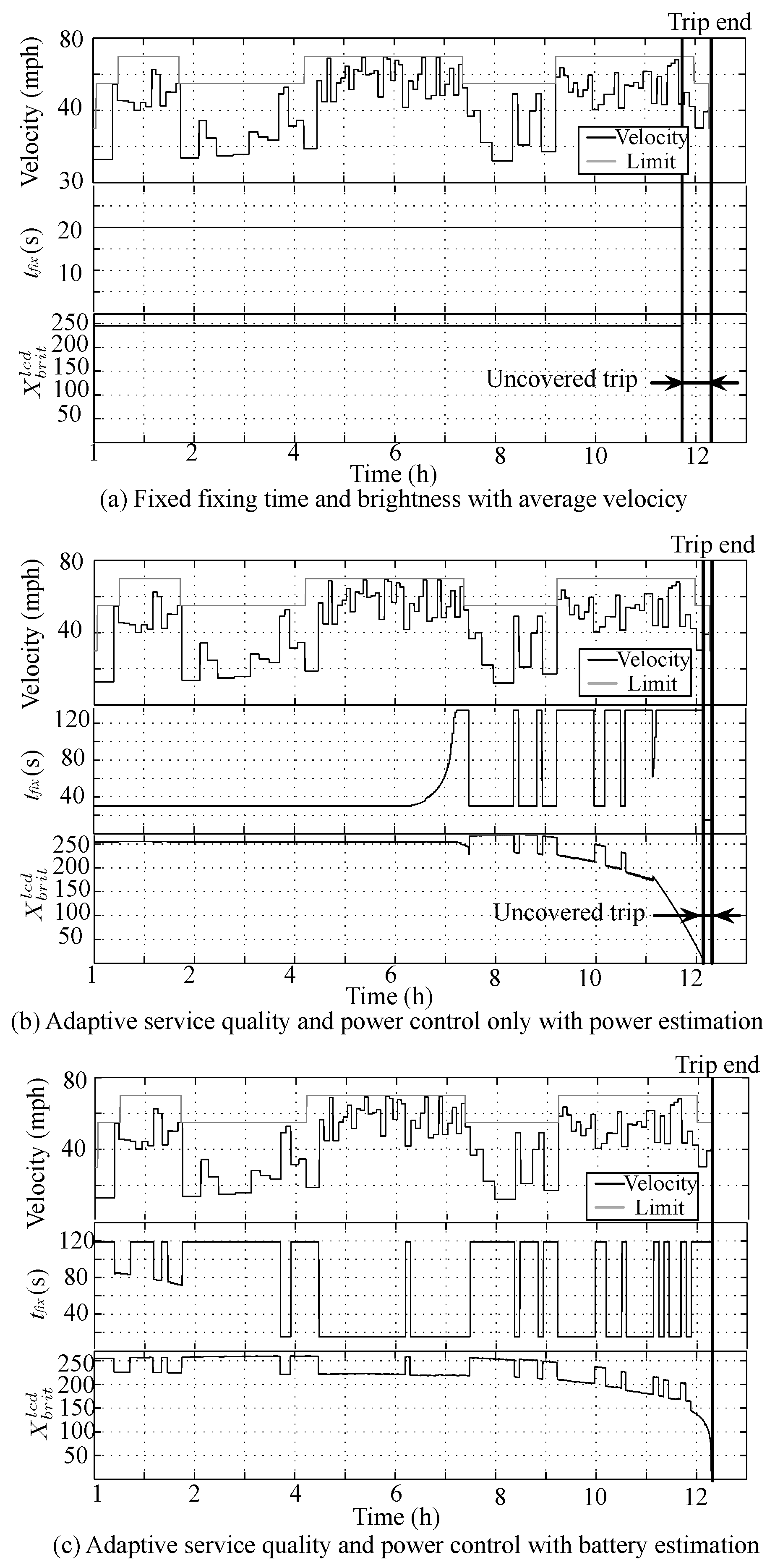
5.2. Adaptive Power and Service Quality Control of a GPS Application with Variable Velocity

The behaviors of ( t f i x , X b r i t l c d ) with the proposed adaptive control method in the battery SOC estimation and power estimation only case are illustrated in Figure 8. We randomly generated a velocity within the upper and lower speed limit range for each time slot for the experiment. We used 2.2139 J for Δ E o t h e r ¯ , while the other simulation parameters were the same as in Section 5.1.
Figure 8 shows the advantage of adaptive control. The battery SOC would be exhausted earlier than the trip end time when we fix t f i x and X b r i t l c d using only the average velocity, as shown in Figure 8a. Figure 8b,c shows that the algorithm tends to decrease t f i x and X b r i t l c d at high velocities in order to maintain the location accuracy. t f i x and X b r i t l c d increase when the velocity is low, and sufficient locating accuracy can be achieved with a relatively long t f i x . Unless we consider the rate-capacity effect of the battery, the phone also fails to complete the trip, as shown in Figure 8b, even if we control t f i x and X b r i t l c d . The proposed algorithm with the battery estimation completes the trip while achieving better service quality.
We integrate Q s e r v i c e over time to compare the results, which is given by:
t = 0 t e n d Q s e r v i c e d t .
We set all weight values, ω 1 , 2 , 3 , to 1 in this experiment. The integrated Q s e r v i c e for a fixed value was 31.38 over time, where 8.9% of the trip was not covered by GPS service time. The integrated Q s e r v i c e of adaptive control in the power estimation only case was 33.61 over time where 4% of the trip was not covered by the GPS service time. The proposed adaptive control method with battery SOC estimation achieved a 34.53 integrated Q s e r v i c e score, where the full trip was covered by the GPS service time. The proposed algorithm with the battery estimation achieved a 10.3% and 2.7% Q s e r v i c e improvement compared with the fixed case and power estimation only cases, respectively.

6. Conclusions

This paper introduced a mobile GPS application design using accurate power estimation and accurate remaining battery charge estimation. The application considers the power consumption of the units of the mobile device such as the CPU, cellular, Wi-Fi, LCD, audio, GPS, vibration motor, and more. We more accurately calculated the power consumption of certain units such as the cellular, Wi-Fi, and GPS components by considering their states. We verified our model by comparing it with real platform measurements using commercially available devices. The result showed that our model provides a much more accurate duration time estimation of mobile devices that use a battery.
We performed a service quality and battery lifetime tradeoff analysis. The results showed that our power-aware design framework helps to achieve maximum service quality while ensuring the task will be completed. We also proposed an adaptive algorithm that deals with velocity variations during a trip monitored by GPS. The proposed adaptive control method that uses our battery SOC estimation ensured that the mobile device fully covers the trip while achieving a 10.3% Q s e r v i c e improvement compared with the same task where a fixed velocity was assumed. In a future study, we hope to extend the proposed battery-aware GPS control design framework to electric vehicles with GPS-based navigation or autonomous driving. We want to increase the accuracy of the estimation given the recent progress in battery SOC estimation, sensor fusion technique, and traffic prediction in future work. We will also compare the evaluation results with conventional techniques and hybrid approaches.

Author Contributions

Conceptualization, J.K. and D.S.; methodology, N.C. and D.S.; software, J.K.; validation, N.C. and D.S.; formal analysis, J.K. and D.S.; investigation, J.K.; resources, N.C.; data curation, J.K.; writing—original draft preparation, J.K.; writing—review and editing, N.C. and D.S.; visualization, J.K.; supervision, D.S.; project administration, D.S.; funding acquisition, J.K. and D.S. All authors have read and agreed to the final version of the manuscript.

Funding

This work was supported by a National Research Foundation of Korea (NRF) grant funded by the Korea government (MSIT) (NRF-2020R1A4A4079859 and NRF-2021R1F1A1060208.

Institutional Review Board Statement

Not applicable.

Informed Consent Statement

Not applicable.

Data Availability Statement

Not applicable.

Conflicts of Interest

The authors declare no conflict of interest.

Abbreviations

GPSGlobal Positioning System
OSOperating System
SOCState of Charge
QOSQuality of Service
OCOpen Circuit
APIApplication Programming Interface
LCDLiquid Crystal Display
CCFLCold Cathode Fluorescent Lamp
LEDLight Emitting Diode
CPUCentral Processing Unit
TFTThin Film Transistor
VMVibration Motor

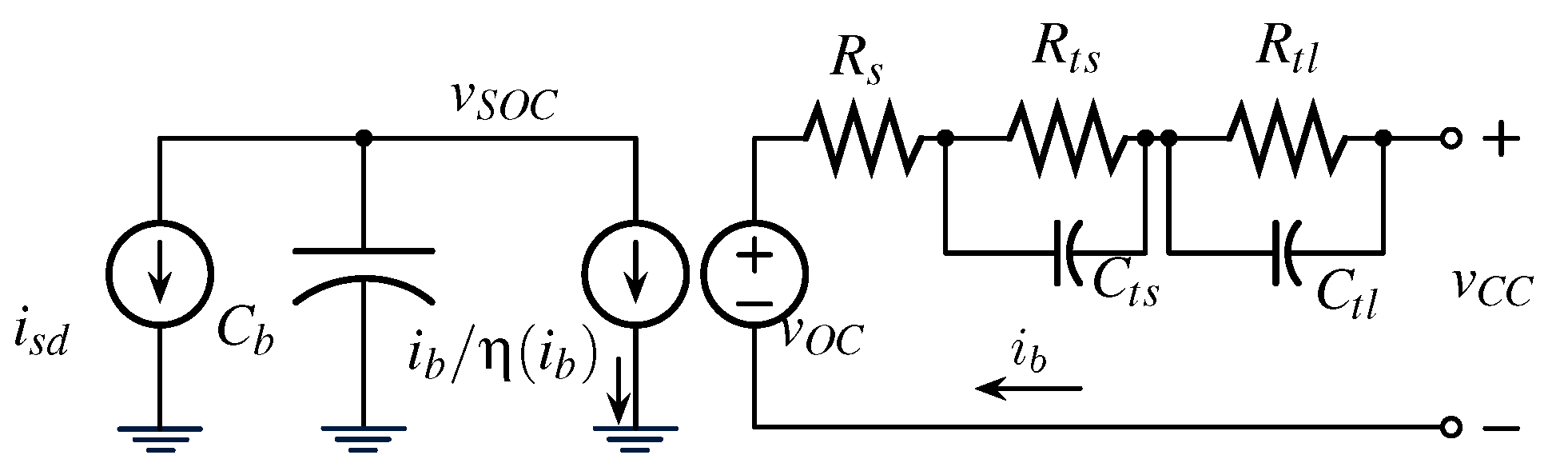
Appendix A. Battery Model

There are many analytical battery models based on electrochemical knowledge [25,26,27,28,29]. However, the complicated analytical battery models are not easy to use for estimating a handheld device’s battery SOC in a real-time environment. Thus, we used circuit-based battery models such as [30,31,32]. We adopt the battery model from [10]. We measured the internal resistance of the target battery as about 100 mΩ, which is not negligible in [10]. In this section, the constructed equivalent circuit model and its parameters are introduced to prevent the overestimation of the remaining battery SOC.

Appendix A.1. Battery Circuit Model

In our previous work [10], we adopted an equivalent circuit battery model from [30]. The equivalent circuit model is depicted in Figure A1. This model enables the run-time and real-time estimation of battery SOC. The remaining charge in the battery is modeled as a capacitor C b , which shows the voltage variance v S O C based on the remaining charge in the battery. v S O C is expressed as follows:
v S O C = C b / C b , f u l l × 1 V ,
where C b , f u l l is the capacity of the battery and C b is the currently stored charge. The open-circuit voltage of a relaxed battery ( v O C ) only relates to its SOC. Thus, v O C is calculated by using v S O C . We ignore the internal capacitance ( C t s and C t l ) of the battery in the hand-held device since the typical charge/discharge current is relatively small. The internal resistances R s , R t s , and R t l are also simplified as R t o t a l using the heuristic. We model the battery using v O C and R t o t a l as follows:
v O C = b 11 e b 12 v S O C + b 13 v S O C 4 + b 14 v S O C 3 + b 15 v S O C 2 + b 16 v S O C + b 17 , R t o t a l = b 21 e b 22 v S O C + b 23 ,
where b 11 b 17 and b 21 b 23 are coefficients extracted by experiments. We also consider the battery discharge current i b , since there is the rate capacity effect where a larger amount of battery discharge current decreases the battery discharging efficiency η ( i b ) . We approximate η ( i b ) as ( i b ) k d using Peukert’s law [33]. We also extract k d by measurement. KPL6072196 Li-ion cell coefficients, b 11 b 17 , b 21 b 23 , and k d are denoted in Table A1.
Figure A1. Li-ion battery equivalent circuit model.
Energies 14 05333 g0a1
Table A1. Extracted parameters of the battery models.
Coeff.ValueCoeff.ValueCoeff.Value
b 11 −0.265 b 12 −61.649 b 13 −2.039
b 14 5.276 b 15 −4.173 b 16 1.654
b 17 3.356 b 21 −0.043 b 22 −14.275
b 23 0.154 k d 0.019

Appendix A.2. Remaining Charge Estimation

We calculate the remaining battery SOC by subtracting the consumed energy Δ E from the previous state’s battery SOC:
E ( t + Δ t ) = E ( t ) Δ E .
The consumed energy Δ E is calculated as:
Δ E = Δ t ( P c p u + P l c d + P g p s + P a u d i o + P c e l l u l a r + P w f + P v m ) + E l o s s .
The power-consuming unit of the smartphone when the GPS application is running consists of a CPU ( P c p u ), display ( P l c d ), positioning ( P g p s ), audio ( P a u d i o ), cellular ( P c e l l u l a r ), Wi-Fi ( P w i f i ), and vibration motor ( P v m ). The energy consumption in a certain period ( Δ t ) is calculated by Δ t Σ P + E l o s s as in Equation (A4), where E l o s s denotes the internal energy loss of the battery. E l o s s is derived from Equation (A2) by summing the ohmic and rate-capacity effect loss as follows:
E l o s s = Δ t ( i b 2 R t o t a l + i b · v O C · ( 1 / η ( i b ) 1 ) ) .

Appendix B. Target Platform Model

Hardkernel’s [21] Odroid-A platform is a high-end smart device development platform that has similar functionalities to Samsung Galaxy S2. We used Odroid-A platform model from [10]. The component units, which compose the Odroid-A platform, are listed in Table A2. We used the activity profiler of Android OS to extract the activity of each unit.
Table A2. The units composing the target platform.
ComponentsModelDescrpition
ProcessorExynos4210Dual-core CPU
cellular moduleF5521GWG + GPS module
Wi-GiGB8632Wi-Fi + bluetooth module
DisplayLP101WH11366 × 768 TFT LCD
Audio codecMAX98089Full-featured codec
Vibration motorDMJBRK36SVibration motor
BatteryKPL607219610 Ah Lithium polymer

Appendix B.1. CPU

We model the power consumption of the CPU using its execution frequency and utilization as:
P c p u = C f r e q c p u X f r e q c p u ( X k e r n e l c p u + X u s e r c p u ) + P 0 c p u ,
where C f r e q c p u and P 0 C P U are coefficients. The CPU execution frequency is denoted in X f r e q c p u . The CPU utilization of kernel and user program are denoted by X k e r n e l c p u and X u s e r c p u , respectively.

Appendix B.2. Cellular Module

The power consumption of the cellular module heavily depends on its running state, which consists of IDLE, FACH, and DCH. Thus, we use the time use rate of each state within a certain period of time.
P c e l l u l a r = X o n c e l l u l a r ( C i d l e c e l l u l a r X i d l e c e l l u l a r + C f a c h c e l l u l a r X f a c h c e l l u l a r + C d c h c e l l u l a r X d c h c e l l u l a r ) ,
where X o n c e l l u l a r is 1 when the cellular module is activated, or 0 otherwise. The use rates of each state are denoted by X i d l e c e l l u l a r , X f a c h c e l l u l a r , and X d c h c e l l u l a r when C i d l e c e l l u l a r , C f a c h c e l l u l a r , and C d c h c e l l u l a r are the coefficients, respectively.

Appendix B.3. Wi-Fi Module

The Wi-Fi module’s power consumption also heavily depends on its running state. Unlike the cellular module, it only has LOW and HIGH running states, representing its wireless link speed. It is modeled using the time use rate of each state as:
P w f = X o n w f ( C l o w w f X l o w w f + C h i g h w f X h i g h w f ) .
We assume that the Wi-Fi module only consumes power when it is turned on ( X o n w f ). X l o w w f and X h i g h w f are the time uss of each state. C l o w w f and C h i g h w f are the coefficients.

Appendix B.4. Display

The LCD consists of a display device and its control module. The control module always consumes electricity even the display is fully turned off. The display device typically consumes electricity proportional to its brightness. The constant value P c t r l l c d denotes the consumed electricity of the control module. As a fully turned off display device does not consume electricity at all, we set a variable X o n l c d to represent this. When the display device is at full brightness, it consumes much more electricity than when it is at other brightness levels. Thus, we use the time utilization rate when it is in full brightness or not ( X f u l l l c d and X b r i t l c d , respectively). We consequently model the LCD as:
P l c d = P c t r l l c d + X o n l c d ( C f u l l l c d X f u l l l c d + C b r i t l c d X b r i t l c d ) + P 0 l c d ,
where C b r i t l c d , C f u l l l c d , and P 0 l c d are the coefficients.

Appendix B.5. Audio Device

We assume that the audio device does not consume power at all when it is not activated ( X o n a u d is 1 or 0). Otherwise, it consumes power proportional to the volume. We model audio devices as:
P a u d = X o n a u d ( C v o l a u d X v o l a u d + C o n a u d ) ,
X v o l a u d , C v o l a u d , and C o n a u d are coefficients.

Appendix B.6. GPS Module

As with a cellular module, the GPS module has OFF, SLEEP, and ACTIVE states. Each state consumes a different amount of power. Thus, we adopt the time utilization rate for each state ( X o f f g p s , X s l e e p g p s , and X a c t i v e g p s ). The GPS module does not consume power when it is inactive ( X o n g p s is 1 or 0). Thus, we describe the power model of GPS as:
P g p s = X o n g p s ( C o f f g p s X o f f g p s + C s l e e p g p s X s l e e p g p s + C a c t i v e g p s X a c t i v e g p s ) ,
where C o f f g p s , C s l e e p g p s , and C a c t i v e g p s are the coefficients.

Appendix B.7. Vibration Motor

The vibration motor consumes different amounts of power depending on its vibration strength and patterns. Still, we assume it consumes average constant power when activated since its vibration strength and patterns are typically fixed. We describe the power model of vibration motor as:
P v m = C o n m o t o r X o n m o t o r ,
where C o n m o t o r is the coefficient. X o n m o t o r denotes whether the motor is activated or not. We finally present the extracted coefficients of the Android system power model in Table A3.
Table A3. The extracted coefficients of the Android system power model.
ComponentCoeff.ValueCoeff.Value
Processor C f r e q c p u 0.00642 P 0 c p u 0.332
Cellular C i d l e c e l l u l a r 0.011 C d c h c e l l u l a r 0.672
C f a c h c e l l u l a r 0.322
Wi-fi C h i g h w f 0.020 C l o w w f 0.740
Display C b i r t l c d 0.004 P 0 l c d 0.224
C f u l l l c d 1.307 P c t r l l c d 0.067
Audio C o n a u d 0.024 C v o l a u d 0.00009
Vibration motor C o n v i b 0.003
GPS C o f f G P S 0.011 C a c t i v e G P S 0.212
C s l e e p G P S 0.069

References

  1. Shye, A.; Scholbrock, B.; Memik, G. Into the wild: Studing real user activity patterns to guide power optimizations for mobile architectures. In Proceedings of the 2009 42nd Annual IEEE/ACM International Symposium on Microarchitecture (MICRO), New York, NY, USA, 12–16 December 2009; pp. 168–178. [Google Scholar]
  2. Dong, M.; Zhong, L. Sesame: A self-constructive virtual power meter for battery-powered mobile systems. In Proceedings of the 9th International Conference on Mobile Systems, Applications, and Services (MobiSys 2011), Bethesda, MD, USA, 28 June– 1 July 2011. [Google Scholar]
  3. Zhang, L.; Tiwana, B.; Dick, R.P.; Wang, Z.; Mao, Z.M.; Qian, Z.; Yang, L. Accurate Online Power Estimation and Automatic Battery Behavior Based Power Model Generation for Smartphones. In Proceedings of the 2010 IEEE/ACM/IFIP International Conference on Hardware/Software Codesign and System Synthesis (CODES+ISSS), Scottsdale, AZ, USA, 24–29 October 2010. [Google Scholar]
  4. Bian, X.; Wei, Z.; He, J.; Yan, F.; Liu, L. A Two-Step Parameter Optimization Method for Low-Order Model-Based State-of-Charge Estimation. IEEE Trans. Transp. Electrif. 2021, 7, 399–409. [Google Scholar] [CrossRef]
  5. Wei, Z.; Hu, J.; He, H.; Li, Y.; Xiong, B. Load Current and State-of-Charge Coestimation for Current Sensor-Free Lithium-Ion Battery. IEEE Trans. Power Electron. 2021, 36, 10970–10975. [Google Scholar] [CrossRef]
  6. Hu, J.; He, H.; Wei, Z.; Li, Y. Disturbance-Immune and Aging-Robust Internal Short Circuit Diagnostic for Lithium-Ion Battery. IEEE Trans. Ind. Electron. 2021. early access. [Google Scholar] [CrossRef]
  7. Kim, Y.; Park, S.; Cho, Y.; Chang, N. System-Level Online Power Estimation using an On-Chip Bus Performance Monitoring Unit. IEEE Trans. Comput.-Aided Des. Integr. Circ. Syst. (TCAD) 2011, 30, 1585–1598. [Google Scholar]
  8. Gurun, S.; Krintz, C. A run-time, feedback-based energy estimation model for embedded devices. In Proceedings of the 4th International Conference on Hardware/Software Codesign and System Synthesis, Seoul, Korea, 22–25 October 2006; pp. 28–33. [Google Scholar]
  9. Majima, T.; Yokoyama, T.; Zeng, G.; Kamiyama, T.; Tomiyama, H.; Takada, H. Modeling Power Consumption of Applications in Wireless Communication Devices Using OS Level Profiles. In Proceedings of the International SoC Design Conference, Busan, Korea, 22–24 November 2009. [Google Scholar]
  10. Shin, D.; Lee, W.; Kim, K.; Wang, Y.; Xie, Q.; Pedram, M.; Chang, N. Online Estimation of the Remaining Energy Capacity in Mobile Systems Considering System-Wide Power Consumption and Battery Characteristics. In Proceedings of the Asia South Pacific Design Automation Conference (ASP-DAC), Yokohama, Japan, 22–25 January 2013. [Google Scholar]
  11. Navsys Corporation. Low–Power GPS Applications. Available online: http://www.navsys.com/ (accessed on 26 August 2021).
  12. Chen, K.; Tan, G.; Cao, J.; Lu, M.; Fan, X. Modeling and Improving the Energy Performance of GPS Receivers for Location Services. IEEE Sens. J. 2020, 20, 4512–4523. [Google Scholar] [CrossRef]
  13. Raskovic, D.; Giessel, D. Battery-Aware Embedded GPS Receiver Node. In Proceedings of the 2007 Fourth Annual International Conference on Mobile and Ubiquitous Systems: Networking & Services (MobiQuitous), Philadelphia, PA, USA, 6–10 August 2007; pp. 1–6. [Google Scholar]
  14. Thiagarajan, A.; Ravindranath, L.; LaCurts, K.; Madden, S.; Balakrishnan, H.; Toledo, S.; Eriksson, J. VTrack: Accurate, Energy-aware Road Traffic Delay Estimation Using Mobile Phones. In Proceedings of the 7th ACM Conference on Embedded Network Sensor Systems (SenSys09), Berkeley, CA, USA, 4–6 November 2009. [Google Scholar]
  15. KhademSohi, H.; Sharifian, S.; Faez, K. Accuracy-energy optimized location estimation method for mobile smartphones by GPS/INS data fusion. In Proceedings of the 2016 2nd International Conference of Signal Processing and Intelligent Systems (ICSPIS), Tehran, Iran, 14–15 December 2016. [Google Scholar]
  16. Alemneh, E.; Senouci, S.; Brunet, P. An Energy Efficient Smartphone Sensors’ Data Fusion for High Rate Position Sampling Demands. In Proceedings of the 2019 16th IEEE Annual Consumer Communications Networking Conference (CCNC), Las Vegas, NV, USA, 11–14 January 2019. [Google Scholar]
  17. Brown, A.; Brown, P.; Griesbach, J.; Boult, T. A Wireless GPS Wristwatch Tracking Solution. In Proceedings of the SDR Forum 2006, Fort Worth, TX, USA, 26–29 September 2006. [Google Scholar]
  18. Sottile, E.; Giacchetti, T.; Tuveri, G.; Piras, F.; Calli, D.; Concas, V.; Zamberlan, L.; Meloni, I.; Carrese, S. An innovative GPS smartphone based strategy for university mobility management: A case study at the University of RomaTre, Italy. Res. Transp. Econ. 2021, 85, 100926. [Google Scholar] [CrossRef]
  19. Danko, M.; Hanko, B.; Drgoňa, P. Optimized Control of Energy Flow in an Electric Vehicle based on GPS. Commun. Sci. Lett. Univ. Zilina 2021, 23, C7–C14. [Google Scholar] [CrossRef]
  20. Chang, N.; Choi, I.; Shim, H. DLS: Dynamic Backlight Luminance Scaling of Liquid Crystal Display. IEEE Trans. Very Large Scale Integr. Syst. (TVLSI) 2004, 12, 837–846. [Google Scholar] [CrossRef]
  21. Hardkernel, Co. Ltd. Odroid-A Platform. Available online: http://www.hardkernel.com (accessed on 26 August 2021).
  22. Texas Instruments, Co. Ltd. INA194 Current Sense Amplifier. Available online: https://www.ti.com/product/INA194 (accessed on 26 August 2021).
  23. National Instruments Co. National Instruments. Available online: https://www.ni.com (accessed on 26 August 2021).
  24. Agilent Co. Agilent E3631 Power Supply. Available online: https://www.keysight.com/us/en/product/E3631A (accessed on 26 August 2021).
  25. Rong, P.; Pedram, M. An analytical model for predicting the remaining battery capacity of Lithium-ion batteries. IEEE Trans. Very Large Scale Integr. Syst. 2006, 14, 441–451. [Google Scholar] [CrossRef]
  26. Moura, S.J.; Argomedo, F.B.; Klein, R.; Mirtabatabaei, A.; Krstic, M. Battery State Estimation for a Single Particle Model with Electrolyte Dynamics. IEEE Trans. Control Syst. Technol. 2017, 25, 453–468. [Google Scholar] [CrossRef]
  27. Chen, N.; Zhang, P.; Dai, J.; Gui, W. Estimating the State-of-Charge of Lithium-Ion Battery Using an H-Infinity Observer Based on Electrochemical Impedance Model. IEEE Access 2020, 8, 26872–26884. [Google Scholar] [CrossRef]
  28. Zheng, L.; Zhu, J.; Wang, G.; Lu, D.D.; He, T. Lithium-ion Battery Instantaneous Available Power Prediction Using Surface Lithium Concentration of Solid Particles in a Simplified Electrochemical Model. IEEE Trans. Power Electron. 2018, 33, 9551–9560. [Google Scholar] [CrossRef]
  29. Rakhmatov, D. Battery voltage modeling for portable systems. ACM Trans. Des. Autom. Electron. Syst. 2009, 14, 1–36. [Google Scholar] [CrossRef]
  30. Chen, M.; Rincon-Mora, G. Accurate electrical battery model capable of predicting runtime and I–V performance. IEEE Trans. Energy Convers. 2006, 21, 504–511. [Google Scholar] [CrossRef]
  31. Ruan, H.; He, H.; Wei, Z.; Quan, Z.; Li, Y. State of Health Estimation of Lithium-ion Battery Based on Constant-Voltage Charging Reconstruction. IEEE J. Emerg. Sel. Top. Power Electron. 2021. early access. [Google Scholar] [CrossRef]
  32. Benini, L.; Castelli, G.; Macii, A.; Macii, E.; Poncino, M.; Scarsi, R. Discrete-time battery models for system-level low-power design. IEEE Trans. Very Large Scale Integr. Syst. 2001, 9, 630–640. [Google Scholar] [CrossRef]
  33. Linden, D.; Reddy, T.B. Handbook of Batteries; McGrew-Hill Professional: New York, NY, USA, 2001. [Google Scholar]
Figure 1. Energy-aware application design framework.
Energies 14 05333 g001
Figure 2. GPS service quality model: (a) smaller locating error with a shorter fix period, (b) larger locating error with a longer fix period, and (c) total trip path and its estimation time.
Energies 14 05333 g002
Figure 3. The GPS consumes a different amount of power depending on its state. (a) GPS power consumption has a typical pattern based on its state. (b) GPS state analysis. After initialization, it consumes meagre power when it enters the OFF state.
Energies 14 05333 g003
Figure 4. LCD brightness and power consumption.
Energies 14 05333 g004
Figure 5. Variable velocity and fixing time interval: (a) the speed limit along the trip and (b) each fixing time interval.
Energies 14 05333 g005
Figure 6. Experimental setup.
Energies 14 05333 g006
Figure 7. The maximum Q s e r v i c e is different under different assumptions: (a) slightly higher maximum Q s e r v i c e since it does not consider internal battery loss (not a practical case); (b) a more realistic case considering battery internal loss.
Energies 14 05333 g007
Figure 8. Behavior of ( t f i x , X b r i t l c d ) for (a) fixed values with average velocity, (b) service quality control only with power estimation, and (c) with battery estimation.
Energies 14 05333 g008
Table 1. Nomenclature.
SymbolDescriptionSymbolDescription
ϵ maximum locating error of the GPSvvelocity of GPS tracking object
t f i x fixing period of the GPS ϵ 0 fundamental GPS error
t a c t i v e duration of the ACTIVE state of the GPS t g o o f f duration of the SLEEP state of the GPS
t t o t a l period of one GPS activation cycle C o v e r a g e normalized trip coverage
t s e r v i c e service time (battery lifetime) t t r i p given trip time
Δ E G P S ¯ energy used in the GPS module in a certain period Δ t time period
C o f f G P S , C s l e e p G P S , C a c t i v e G P S power coefficients of the GPS X o f f G P S duration ratio of the OFF state of the GPS
X s l e e p G P S duration ratio of the SLEEP state of the GPS X a c t i v e G P S duration ratio of the ACTIVE state of the GPS
Δ E o t h e r ¯ energy used by other devices in the smartphone E l o s s internal energy loss of the battery
v O C open-circuit voltage of the battery Q l c d quality of service of LCD
X b r i t l c d brightness of the LCD Q s e r v i c e quality of service of the application (system)
ω 1 , ω 2 , ω 3 Weight values to calculate Q s e r v i c e R t o t a l battery internal resistance
Publisher’s Note: MDPI stays neutral with regard to jurisdictional claims in published maps and institutional affiliations.

