Development of Advanced Smart Ventilation Controls for Residential Applications

Abstract

This study examined the use of zoned ventilation systems using a coupled CONTAM/EnergyPlus model for new California dwellings. Several smart control strategies were developed with a target of halving ventilation-related energy use, largely through reducing dwelling ventilation rates based on zone occupancy. The controls were evaluated based on the annual energy consumption relative to continuously operating non-zoned, code-compliant mechanical ventilation systems. The systems were also evaluated from an indoor air quality perspective using the equivalency approach, where the annual personal concentration of a contaminant for a control strategy is compared to the personal concentration that would have occurred using a continuously operating, non-zoned system. Individual occupant personal concentrations were calculated for the following contaminants of concern: moisture, CO₂, particles, and a generic contaminant. Zonal controls that saved energy by reducing outside airflow achieved typical reductions in ventilation-related energy of 10% to 30%, compared to the 7% savings from the unzoned control. However, this was at the expense of increased personal concentrations for some contaminants in most cases. In addition, care is required in the design and evaluation of zonal controls, because control strategies may reduce exposure to some contaminants, while increasing exposure to others.

1. Introduction

Available options for reducing the energy impact of ventilation in homes have included demand-controlled ventilation (DCV) systems that ventilate based on CO₂ sensing, as well as heat and energy recovery ventilation systems. A meta-analysis of 38 studies of residential DCV [1] concluded that, while energy savings can be significant (up to 60%), there is a lot of variability, including energy increases of up to 26%. In addition, building and material-related contaminants (i.e., volatile organic compounds (VOCs)) are ignored in current DCV approaches. A sole focus on CO₂ has allowed these controls to appear robust on the surface, while ignoring important contaminant exposures in homes (e.g., formaldehyde, combustion pollutants). In residences, there are a few DCV approaches that also include humidity control. Heat and energy recovery ventilation has substantial potential energy savings, but costs are high, and the maintenance requirements and challenging installation remain barriers to widespread adoption. Smart ventilation is a low-cost alternative. It uses simple and inexpensive ventilation fans combine with controls to vary the time and quantity of ventilation, while maintaining indoor air quality equivalent to traditional code-compliant systems.

The initial principles behind “Smart Ventilation” were developed to account for exposures to building-related contaminants in residential ventilation controls, based on the concept of “equivalence” [2,3]. Equivalence is defined as the condition where a variable air flow ventilation system provides the same annual exposure to a generic, continuously emitted contaminant as a continuously operating system. The relative exposure metric operationalizes the concept of equivalence, and its calculation methods [4] have been integrated into the ASHRAE 62.2 ventilation standard in 2016, which provides a path to compliance with the standard that includes ventilation controls providing equivalent exposure (i.e., relative exposure <= 1).

Subsequent efforts have applied these concepts in developing smart ventilation controls, based largely on simulation efforts, but also some limited field research [5]. The equivalence principle was first used in the development of the RIVEC controller (short for Residential Integrated VEntilation Controller), which was developed and briefly field-tested in California. RIVEC used occupancy and local exhaust fan sensing, along with grid signals and timer-based temperature controls [6]. Additional research has developed and demonstrated the performance of smart controls based on outdoor temperature [4,7], indoor humidity control [8], as well as occupancy and local exhaust controls [9,10]. Recent work in Florida has documented the performance of a multi-parameter optimized control for both outdoor temperature and humidity [11]. In addition to mechanical ventilation controls, related efforts have addressed passive stack and hybrid ventilation equipment [12]. Most of these efforts have focused on achieving annual energy savings, but others have extended the analysis of smart ventilation to examine peak power reductions in homes, showing that residences in California had the potential for up to 0.2 W/ft² (20 W/m²) or up to 30% of total home power demand during peak periods [13].

The majority of these efforts have addressed new, energy efficient construction, using the assumption of a single well-mixed zone in the dwelling. They have relied solely on a continuously emitted, generic contaminant, with a constant dwelling ventilation flow as the reference case. For zonal dwellings, the simplifying assumption of a single well-mixed zone does not apply. This study builds on these previous efforts using the same ventilation equivalence principles described above, but applied in a multi-zone context, where the dwelling is an assemblage of multiple well-mixed zones (e.g., kitchen, living room). The focus is on ventilation systems that can ventilate part of a home, while not ventilating others (i.e., zonal ventilation).

A key aspect of the current work is that the control strategies studied here are explicitly designed to include both energy savings and Indoor Air Quality (IAQ) calculations that account for the dynamics of indoor concentrations for key contaminants of concern to human health. Accordingly, our analysis includes contaminants related to occupancy (that vary spatially and temporally), as well as generic, continuously-emitted contaminants. We separately assess the impacts of zoning constant flow ventilation systems and the impacts of zonal smart controls. The comparisons were done in two parts. First, we compared baseline continuously operating ventilation systems that exhausted or supplied to/from a single location versus zoned systems that supplied or exhausted to/from multiple locations in each dwelling. Then, we evaluated zonal smart ventilation controls compared to continuous operation of the same multi-location ventilation systems. Energy and airflow modeling tools are used to explore these issues. More details of these tools can be found in [14].

2. Multi-Zone Smart Ventilation Control

For our assessment and development of zonal ventilation controls, we adapted the equivalence and relative exposure approaches used in ASHRAE 62.2 to a zonal context, and we applied them to individual occupants, rather than the building itself. We also expanded the concept to include both a generic VOC contaminant and specific contaminants of concern (i.e., CO₂, PM_2.5, and water vapor). Each contaminant had their own scheduled emissions, sources, and removal mechanisms, which are described in detail below. We use personal contaminant concentrations to extend the equivalence concept to individual occupants and specific contaminant species rather than just the spaces themselves. This approach uses personal concentration ratio as its core metric of comparison. This allows the control strategies to account for occupants moving between zones and being absent from the building, while maintaining the core principle of comparing a dynamically controlled ventilation scheme against continuously operating non-zoned systems. The personal concentration ratio is calculated as the ratio of the annual mean personal contaminant concentrations between the smart control and non-controlled baseline case. This ratio was calculated for every contaminant and every occupant. As with single zone-based relative exposure, the ratio of the annual average personal concentrations was used to evaluate the different ventilation approaches. The personal concentration ratios were calculated in post-processing, as they rely on the outputs of the co-simulation mass balance, which fully accounts for all air flows and contaminant transport. It is not practical for a ventilation system controller to know this information.

In making real-time zone control decisions, the controllers use one of two different approaches to estimate real-time air quality.

First, some controls use equivalence calculations to estimate the zone relative exposure, which is used to turn ventilation fans on and off (or modulate their flows). In each zone, the calculations use two flows: (1) an estimate for the real-time total zone ventilation flow (i.e., a combination of zone fan and zone infiltration flows, ignoring inter-zonal flow), and (2) a constant zone reference ventilation flow that is proportional to the zone’s floor area. These two flows are used to calculate the real-time zone relative exposure. This approach effectively treats each zone as a whole dwelling in the calculation of relative exposure. Some controls use the 24-h running average of this zone relative exposure for control purposes.

Second, some controls use the real-time generic contaminant concentration predicted in each zone by CONTAM, which is compared to the whole dwelling steady-state concentration that would occur at the ASHRAE 62.2 target ventilation rate. This value is termed the generic zone relative exposure. Again, some controls also use a 24-h integrated value of generic zone relative exposure.

As occupants move from zone-to-zone, some controls track their time-integrated personal relative exposures. These are assembled based on the time-series of zone relative exposures where the occupant was at each time-step. In addition, some controls track the 24-h running average of the personal relative exposure, which ensures that a person’s high zone relative exposure in one location (e.g., in the kitchen while cooking) can be compensated for with increased ventilation flow when the occupant is in another zone. This type of control would require full awareness of the location of each individual in the home at all times.

Smart Control Descriptions

The smart ventilation strategies modulate ventilation rates throughout the course of a day or year and for different rooms (or zones) in the home. These strategies may respond to outdoor air temperature, zone occupancy, predicted exposures, and measured indoor contaminants. A thorough review of available smart ventilation strategies that have been previously studied can be found in [1]. The unzoned outdoor temperature control (VarQ) varies dwelling ventilation rates based on outdoor temperature to lower ventilation rates when outdoor temperatures are high or low, and has been found to work well in previous investigations in [4,10]. All the other controls are novel zoned controls developed for this study. Ten smart ventilation controls were assessed in three categories:

• Baseline + Indoor Air Quality (IAQ) Controls—Intended to improve IAQ while not affecting energy use, these controls do not modulate the total air flow, instead they change which zone(s) the air is supplied to or exhausted from based on occupancy. They are referred to as ‘tracker’ controls, because flows track zone occupancy. They do not use relative exposure calculations to make control decisions.

  ◦

  supplyTracker—For supply and balanced systems only. When the dwelling is vacant, all fan flows are directed to zones proportional to the zone floor area. When the dwelling is occupied the supply air flows are directed to occupied zones, proportional to the number of occupants in each zone. It is possible for a single occupied zone to receive the full dwelling air flow rate.

  ◦

  occupantTracker—Same as the supply tracker, but for exhaust fans, such that the exhaust flows are from each zone according to floor area when the home is vacant, and from each zone according to number of occupants when the home is occupied.

• Outdoor Temperature Controls—These controls use measured outdoor temperatures to shift ventilation flows to mild weather periods. They require pre-optimization to determine how to best scale outside flows with temperature in each dwelling and location. We performed a pre-optimization for all three of the controllers below. All temperature-based controllers operated on real-time zone relative exposure calculations.

  ◦

  varQ—This controller has been found to be highly effective in previous studies. For unzoned systems, the whole dwelling IAQ fan flow rate is varied according to outdoor dry-bulb temperature, using pre-optimized temperature scaling factors. This leads to increased annual ventilation flow.

  ◦

  varQmzSingleZoneOpt—This controller combines the temperature-based air flow changes of VarQ with occupancy sensing and zonal ventilation equipment. This control has the same airflow at each time-step as the varQ, but fan airflows are directed to occupied zones only proportional to the number of occupants in each zone. This leads to increased annual ventilation flow.

  ◦

  varQmz—For zoned systems, this control has the same calculation procedures as varQ, but temperature scaling parameters are optimized for a two-zone dwelling, using assumed occupancy patterns. This approach can decrease annual ventilation flow.

• Zone Occupancy Controls—These controls modulate the total dwelling air flow in response to zone occupancy. The total dwelling air flow is apportioned to each zone based on floor area (when the dwelling is vacant) or based on occupancy (when the dwelling is occupied). For example, if total dwelling air flow is 100 L/s and a zone is 25% of the dwelling floor area then it is assigned 25 L/s during periods of house vacancy. Similarly, if a dwelling has four occupants and three of them are in a single zone, then this zone receives 75% of the dwelling airflow. Each zone is ventilated at a minimum flow rate when unoccupied. These strategies reduce annual ventilation airflow for the dwelling. Controls use either instantaneous and 24-h averaged zone relative exposure, personal relative exposure, or actual generic contaminant predictions.

  ◦

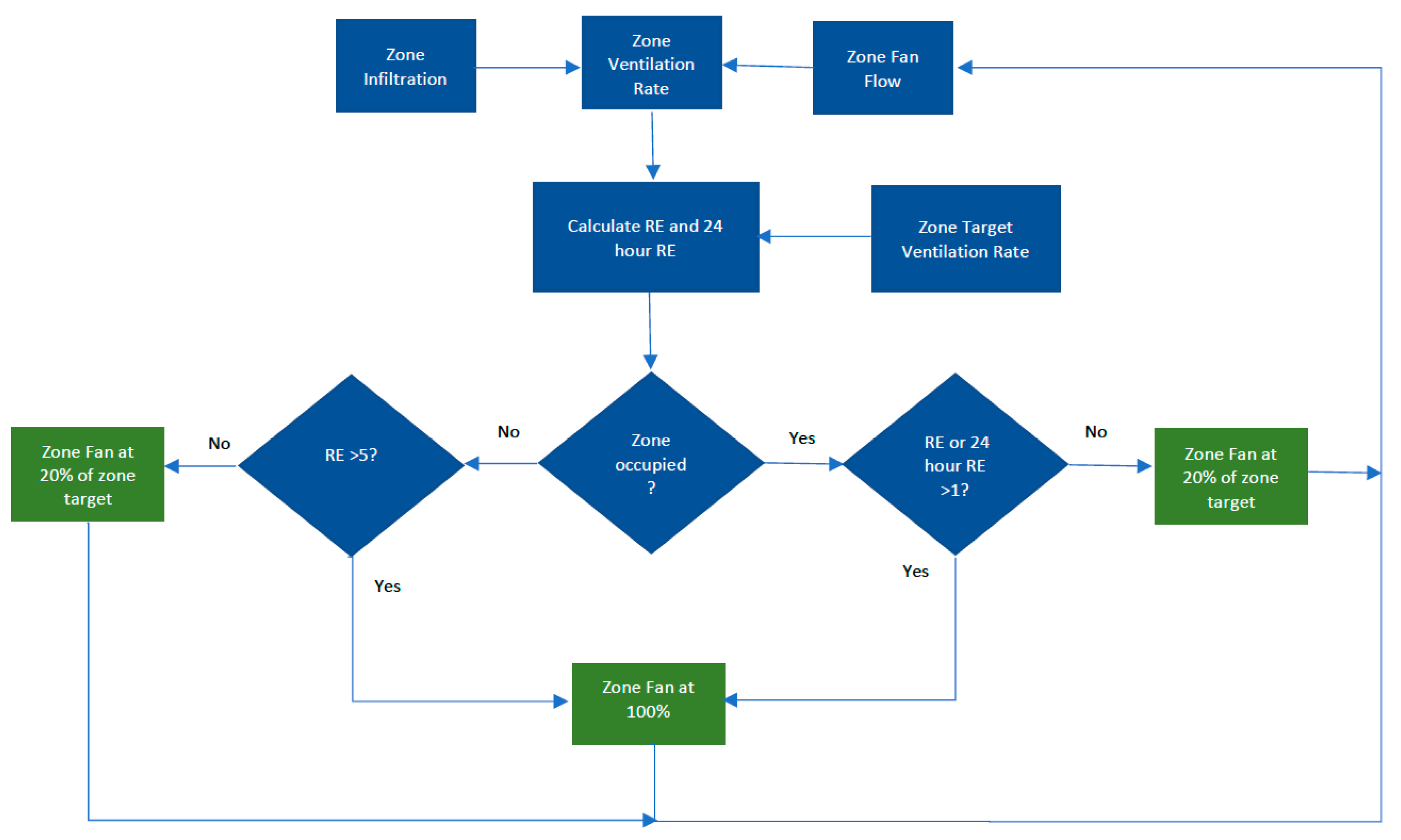
  zoneExposure—Tracks the instantaneous and 24-h averaged zone relative exposure in each zone, and operates the IAQ fan to maintain both metrics below 1 in any zone that is occupied. When vacant, zone relative exposure is controlled to less than 5 to avoid exposure to high contaminant concentrations upon entering a previously unoccupied zone. Figure 1 shows an illustrative flow chart for this zonal controller.

  ◦

  zoneASHQexposure—Same control strategy as zoneExposure, but instead of using controller estimates of instantaneous and 24-h averaged zone relative exposure, it controls the zone generic contaminant concentration (ASHQ) to be the same as the steady-state zone concentration that would occur at the uncontrolled continuous ventilation rate.

  ◦

  occExposure—Tracks controller estimated zone relative exposure in each zone and 24-h averaged personal relative exposure for each occupant. Zones are vented if any person in the zone has a 24-h averaged personal relative exposure greater than 1, or if the zone relative exposure is greater than 1. Unoccupied zone relative exposure is controlled to less than 5 to avoid exposure to high contaminant concentrations upon entering a previously unoccupied zone. This controller ensures that a high personal relative exposure in one zone (e.g., in kitchen while cooking) can be compensated for by increased ventilation and lower relative exposure in another zone.

  ◦

  occASHQexposure—This is the same control strategy as occExposure, but instead of using controller estimates of instantaneous and 24-h averaged personal relative exposure, it controls the zone generic contaminant concentration to be the same as the steady-state zone concentration that would occur at the uncontrolled continuous ventilation rate.

  ◦

  occupantVenter—All zones get a minimum flow rate when unoccupied. Additional airflow is distributed to occupied zones according to the occupant count in each zone. There is no tracking of controller estimated of instantaneous and 24-h averaged personal relative exposure or contaminants.

In order to isolate the impacts of code-required, continuously operated mechanical ventilation, two baseline simulations were run for each case: (1) baseNoFan includes infiltration and auxiliary kitchen and bathroom fans, but no whole dwelling mechanical ventilation; and (2) baseFan adds to this a continuously operating ventilation fan sized to ASHRAE 62.2—2016, including infiltration credits for the single-family dwellings. The constant flow baseline cases (baseFan) were run with all fan types, both zonal and non-zonal, including exhaust, supply, and balanced fans. The baseline used for each zonal control evaluation is the one using the same ventilation fan type. Smart controlled ventilation fan capacities were typically double the baseline fan flows, which enables them to compensate for periods of reduced outside airflow with higher air flows when operating. In most cases, the fan airflows used in the smart ventilation systems were 0.085 m³/s, which was selected to roughly correspond with the largest residential ventilation equipment commonly available in the US market. Exceptions to this smart control fan sizing include: (1) occupantTracker, which used identical fan sizing to the baseline cases; (2) occupantVenter, which increased baseline fan sizes by 50%; and (3) varQmz, which used fans sized at 0.065 m³/s in all cases (selected based on pre-optimization calculations).

For the zonal smart controls, each zone was equipped with a fan capable of delivering the whole dwelling airflow (i.e., 0.085 m³/s in most cases). This allowed the whole dwelling flow to be directed to the occupied zone(s). If more than one zone was occupied, the whole dwelling flow was divided amongst those zones proportional to either their floor area fractions or the number of people in each of those zones. In addition, for each smart control type, all zones were ventilated at a minimum flow rate during all time-steps, which was equivalent to 20% of the baseline fan flow multiplied by the zone’s floor area fraction (see

Table 1. Zone floor area and floor area fraction for each prototype.

Zone Name	Single-Family (%)	1-Story (m2)	2-Story (m2)	Apartment (%)	Apartment (m2)
Bedrooms	29%	56	72	37%	30
Wet Rooms (Bath and Laundry)	16%	31	40	8%	6
Common	44%	85	109	44%	35
Kitchen	11%	23	29	11%	9
TOTAL	100%	195	251	100%	81

). At the end of each time-step, a balancing procedure was carried out for all zone fans to ensure that the sum of all controlled fan flows was never allowed to exceed the total dwelling flow (0.085 m³/s except as noted above).

We considered using controls that respond to real-time contaminant concentrations. However, these proved to be impractical primarily because the ventilation rates required to control formaldehyde below acceptable levels is very high and left no scope for energy-conserving controls. This is primarily because typical formaldehyde levels in homes are far in excess of recommended health limits—even with continuously operating mechanical ventilation in homes with low-emitting materials [15]. This is further compounded by formaldehyde emission rates being variable, in particular, they tend to increase as ambient concentrations decrease, resulting in reduced effects of ventilation on lowering concentrations [16]. With the exception of formaldehyde, all contaminants were below regulatory thresholds.

3. Modeling Approach

The zoned ventilation strategies described above were assessed analytically using a co-simulation combining CONTAM and EnergyPlus. CONTAM solved the air flow and contaminant transport problems, while EnergyPlus solved the thermal balance and building loads models. This co-simulation is based on tools provided and validated by NIST [17,18]. All of the analyses use detailed annual simulations at a five-minute time-step of reference buildings with thermal and airflow characteristics consistent with the prescriptive requirements of the 2019 Residential Building Energy code in California [19]. This energy code has specific prototype buildings that we used in this study: a two-story single-family dwelling (251 m²), one-story single-family dwelling (195 m²), and a single apartment unit from the multi-family prototype (81 m²). Each dwelling was split into at least four zones: the kitchen, bathrooms, bedrooms, and common living spaces. The apartment bedrooms were further divided into adult and child bedroom zones. The two-story home had two common living spaces—a common area downstairs and a family room upstairs. The indoor temperatures were the same for all simulation cases, with identical thermostat schedules used throughout.

Some zones are known sources of contaminants. Kitchens are sources of cooking contaminants, including CO₂, NO₂, PM_2.5, and Acrolein. Bathrooms are sources of CO₂, water vapor and VOCs. We released contaminants in those zones based on episodic events, such as cooking and bathing. This allows the simulations to capture the peak contaminants in kitchens and bathrooms that disperse to other zones. Bedrooms were treated as a separate zone, because they are occupied for extended periods of time on a highly predictable basis. All remaining locations were combined into “common” or “family” zones. These represent locations with no particular expected point-source contaminant emissions, and with no predictable continuous occupancy patterns. For the zonal controls, we also investigated controls where the dwelling was split into two zones. The two-zone controls were based on selecting spaces that had the biggest temporal changes in occupancy so as to maximize any zoning impacts (i.e., bedrooms and non-bedroom), because the bedrooms are unoccupied most of the day and only occupied at night. Similarly, the non-bedroom zone was completely unoccupied at night (and during the day on weekdays).

The total conditioned floor area for each prototype was apportioned to each of these zones using mean values estimated for new home construction in the U.S., based on builder surveys developed by the National Association of Home Builders [20]. The floor area and floor area fractions for each zone and prototype are listed in Table 1. For the multi-family apartment prototype, the fractions were adjusted to reflect typical bathroom sizes in a one-bathroom apartment with a very small laundry area with stacked washer/dryer units, as opposed to a laundry room in the single-family. Dimensioned floor plans for each of these three prototype dwelling units can be found in [14].

Three whole-dwelling, single-point, non-zoned ventilation systems (“SP”) were simulated for comparison to three multi-point, zoned systems (“MP”). Example zone fan airflows are shown for an illustrative case in

Table 2. Example zone ventilation fan flows for a one-story, one ACH₅₀ prototype dwelling in CZ1.

	Common (L/s)		Bedroom (L/s)		Kitchen (L/s)		Wet (L/s)		Total Exhaust (L/s)	Total Supply (L/s)
Fan Type	Exh	Sup	Exh	Sup	Exh	Sup	Exh	Sup
SPexhaust	43	0	0	0	0	0	0	0	43	0
SPsupply	0	43	0	0	0	0	0	0	0	43
SPbalanced	0	23	0	15	16	0	22	0	39	39
MPexhaust	19	0	12	0	5	0	7	0	43	0
MPsupply	0	19	0	12	0	5	0	7	0	43
MPbalanced	6	6	11	11	17	17	4	4	39	39

. Fan flows are distributed to each zone proportional to the zone floor areas. The six ventilation fan types included:

• Central exhaust located in the Common living spaces zone (SPexhaust).
• Central supply located in the Common living spaces zone, with MERV13 filtration for the supply air (SPsupply).
• Balanced system, with exhaust flows from Kitchen and Bathroom zones, and supply flows (with MERV 13 filtration) to the Common living spaces and Bedroom zones (SPbalanced).
• Exhaust fans located in each zone of the dwelling, controlled independently (MPexhaust).
• Supply fans located in each zone of the dwelling, controlled independently (MPsupply).
• Balanced supply/exhaust systems located in each zone of the dwelling. Note, this differs from typical balanced systems, which are balanced for the home, but not for each zone in the home. The system studied here is balanced for each zone (MPbalanced).

Whole house target and mechanical fan airflows were calculated using the ASHRAE 62.2—2019 ventilation standard [21]. Target flows for each zone were determined by dividing the whole dwelling flow amongst the zones proportional to their floor area fractions. All ventilation fans assumed a fixed watts per unit flow rate of 436 watts per m³/s based on certified fan performance data from the Home Ventilating Institute directory [22]. For supply ventilation systems the air was tempered with a 3:1 mix of indoor and outdoor air, leading to four times the air flow and four times the fan power. For balanced systems, the fan power was five times that of the exhaust fan, also based on data from the Home Ventilating Industry products directory. Two different heating and cooling approaches were analyzed: a central forced air heat pump with a MERV13 particle filter that tends to mix air between zones, and distributed heat pump systems with no filtration and much less distribution between zones.

3.1. Model Input Parameters

3.1.1. Occupancy

Occupancy was varied according to the number of bedrooms in each prototype dwelling. The apartment, one-story and two-story prototypes included three, four, and five occupants, respectively. Each occupant included heat gains, water vapor emissions from their showering/bathing, along with respiratory emissions of CO₂ and water vapor. The amount of cooking, laundering and dishwashing was the same for all prototypes and did not vary by occupancy. For weekdays the dwelling was unoccupied from 8 a.m. to 5 p.m. On weekends the dwelling was continuously occupied. A fixed schedule of occupant movement between zones at different times of day was imposed that was intended to mimic an actual day (e.g., sleep in the bedroom with door closed, wake up and leave the bedroom, bathe, cook breakfast, leave the dwelling, return home after work/school, cook dinner, etc.). Together with the zone occupancy schedule, activities were scripted within the zones (e.g., person one in the kitchen zone cooking, or person two in the bathrooms taking a shower). The occupancy for each room or zone is the result of on combining the individual occupant schedules. Although there are multiple occupants emitting contaminants, in the rest of this paper we will only present the exposure results for the occupant with the greatest annual personal concentration ratio, i.e., the adult occupant who did the cooking.

3.1.2. CO₂

For outdoor conditions, we assumed a constant concentration of 400 ppm. For indoors, we based emission rates on the analysis provided by the National Institute of Standards and Technology [18] for the modeling of indoor air quality.

• Adult: 10 mg/s (awake); 6.5 mg/s (asleep)
• Child: 6.5 mg/s (awake); 4 mg/s (asleep)

3.1.3. Moisture

For exterior moisture conditions, we used the hourly ambient humidity data from the State of California Building Energy code hourly weather files for each climate region, which were adapted for use in EnergyPlus. Indoor water vapor emissions included constant background emissions along with event-based and occupancy-based emissions using fixed schedules for bathing, cooking, and breathing. Water vapor generation rates are similar to those in NIST publications [17,18]. Emissions for events (e.g., cooking and bathing) and occupants (e.g., breathing) occurred in the room where the occupants were located. As occupants were scheduled to be in different zones, their emissions moved with them. We assumed that kitchens and bathrooms had the requisite local exhaust systems that directly lower the amount of moisture in the dwelling. Studies of capture efficiency for kitchen range hoods [23] has shown that for typical cooking events (i.e., cooking on a front burner) and range hood operation, about half of cooking contaminants are removed by this local exhaust ventilation. Although data is lacking for bathroom exhaust efficacy, we assumed the same effectiveness as for kitchens. Therefore, we reduced these moisture sources by a factor of two. Using total daily emission rates from ASHRAE 160—2016 [24], the background moisture emission was 20 mg/sec, distributed to each zone proportional to floor area. The resulting water vapor emission rates from all sources are:

• Per Adult: 15 mg/s (awake); 9 mg/s (asleep)
• Per Child: 10 mg/s (awake); 6 mg/s (asleep)
• Dishwashing: 130 mg/s
• Cooking: 140 mg/s (half of the total of 280 mg/s due to range hood operation)
• Showering: 330 mg/s (half of the total of 660 mg/s due to bathroom exhaust operation), varied according to occupancy
• Background emission: 20 mg/s

Indoor moisture predictions were made using the EnergyPlus Effective Moisture Penetration Depth (EMPD) model, which provides a two-layer moisture sorption model for materials in each zone, because some studies have shown that it provides better moisture predictions in occupied dwellings compared to single-layer models [25,26].

3.1.4. Particles (PM_2.5)

Particles had both indoor and outdoor sources, and the modeled loss mechanisms included interior deposition, penetration losses (i.e., filtration by the building envelope), air exchange, and media filtration on supply airflows (both ventilation and/or central air handler included MERV13 filters which removed 90% of PM_2.5 at each pass).

Outdoor particle concentrations varied by season and diurnally. We used pre-generated annual hourly ambient PM_2.5 data from the US EPA AQS system, including all national measurement sites for full calendar years of 2013–2018. We estimated the generation of PM_2.5 from the HENGH field study that measured PM_2.5 concentrations near the cooktop/range and outdoors in 70 new California single-family dwellings [27]. Random forest machine learning was used to disambiguate sources between: outdoors, indoor cooking, and ‘other’ indoor particle generation. The decay of indoor PM_2.5 concentrations after cooking events was used to estimated indoor loss rates using a regression model.

Based on this analysis, average emission rates were determined to be 0.0416 mg/s for cooking, and 0.00007 mg/s for other background emissions. The background emissions are those due to other occupant activities, including resuspension from surfaces. Background emissions occurred only in the occupied zones, proportional to the number of awake occupants in each zone at a given timestep. This approach concentrates emissions in the zones where occupants are, rather than spreading them evenly between occupied and unoccupied zones. We assumed that a fan near the cook range captured 50% of the cooking emissions, giving indoor particle net-emission rates of:

• PM_2.5 cooking: 0.0208 mg/s
• PM_2.5 other: 0.00007 mg/s

The HENGH field study is the basis for our estimates of indoor particle generate rates, so it is important to compare the HENGH field study outdoor concentrations to those from the EPA database. The mean outdoor PM_2.5 for the 70 new California homes in the HENGH study was 9 μg/m³. This value falls squarely within the monthly diurnal values derived from our method described above.

3.2. Generic Contaminants

ASHRAE 62.2 and California building regulations use equivalence calculations based on a generic, continuously emitted contaminant that has no other removal mechanisms, other than by ventilation, and no other sources other than the dwelling or zone being studied. Using this type of generic contaminant gives us an IAQ performance benchmark, that allows for comparison to non-zonal approaches discussed here and in previous studies. The generic contaminant emission rate was 18 μg/m²/h, where the area of each zone determined the mass emission rate.

3.3. Envelope Leakage

Although this study focuses on control of mechanical ventilation systems, we also included the effects of natural infiltration. We restricted the study to relatively tight building envelopes because these will have significant contributions from mechanical ventilation systems, thus emphasizing the effect of the various control strategies. The single-family dwellings had leakage levels of 0.6, 2, and 3 ACH₅₀ (Air Changes per Hour at 50 Pa). The apartment dwellings were simulated only at one envelope leakage level (3 ACH₅₀)–with all of this leakage in the exterior envelope. The internal apartment surfaces were assumed to have zero leakage (they also were assumed to be adiabatic for heat transfer calculations).

3.4. Weather

To cover a wide range of weather conditions, we used four California climate regions (1, 3, 10, and 16), ranging from temperate coastal (CZs 1 and 3), through hot inland (CZ 10) to the colder and dry mountain regions (CZ16). The weather data is based on the CBECC-Res weather files used to demonstrate compliance with California’s Title 24 Building Energy Code [19].

4. Results

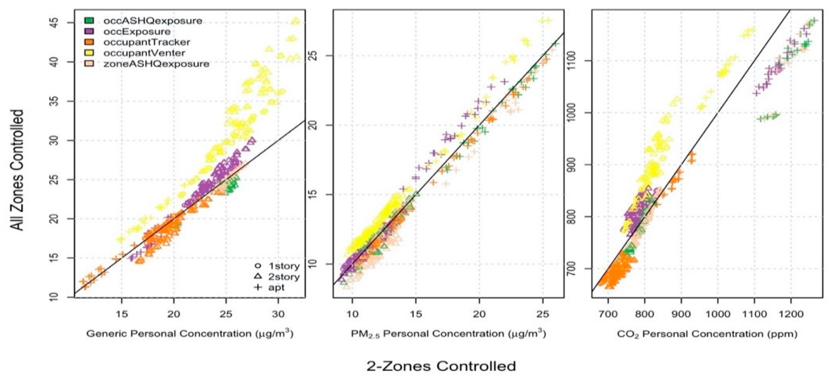
4.1. Impacts of Zoned Ventilation Configurations

In order to distinguish the effects of zonal controls from the zoning of ventilation itself, we compared systems where air was supplied or exhausted from single locations against zoned systems where the air was supplied and exhausted from multiple locations corresponding to the different zones in each dwelling. These baseline cases had constant air flows and no controls. For an example case, Figure 2 shows the average annual diurnal differences in instantaneous personal concentrations for each ventilation fan type when the single location system’s concentrations are subtracted from the zoned system concentrations. Positive values indicate that the zoned configuration increased personal exposure relative to the single location case. During the daytime period from 9 a.m. to 5 p.m., the dwelling is vacant, so no personal concentrations are recorded. The general trend we observe in comparing baseline, constant flow cases is that zonal systems result in lower CO₂ exposures during sleeping hours in bedrooms (green line), but higher exposures during waking hours in other zones for all contaminants.

The time-series plots in Figure 2 are illustrative for a single prototype dwelling in a single location (one-story dwelling, 3 ACH₅₀, CZ10). To further examine zoning effects, all baseline constant flow cases are aggregated and averaged by dwelling prototype and fan type in

Table 3. Annual average results comparing zoned and single-point ventilation configurations for baseline constant flow cases. Highlighted cells show changes greater than +/−5%.

Fan Type	Prototype	Generic			PM2.5			CO2				RH > 60%
		Single-Point Concentration (μg/m3)	Zoned-SP	Change (%)	Single-Point Concentration (μg/m3)	Zoned-SP	Change (%)	Single-Point Concentration (ppm)	Zoned-SP	Change (%)	Change (%) from 400 ppm Baseline	Single-Point RH > 60% (Zone Hours)	Zoned-SP	Change (%)
Balanced	1-story	18.5	0.83	4%	11.5	0.16	1%	753	−8	−1%	−2%	415	95	23%
	2-story	20.5	0.75	4%	12.2	0.07	1%	774	2	0%	1%	156	48	31%
	Apt	12.7	1.24	10%	20.1	0.60	3%	1021	42	4%	7%	227	70	31%
Exhaust	1-story	20.0	0.13	1%	12.0	0.28	2%	783	−27	−3%	−7%	557	−51	−9%
	2-story	25.0	−2.11	−9%	11.4	1.32	11%	904	−84	−9%	−17%	312	−69	−22%
	Apt	12.9	0.15	1%	21.9	0.22	1%	1030	−13	−1%	−2%	304	−18	−6%
Supply	1-story	22.7	−1.30	−6%	11.8	0.21	2%	772	−3	0%	−1%	557	12	2%
	2-story	25.3	−2.33	−9%	12.5	0.17	1%	813	−24	−3%	−6%	170	65	38%
	Apt	18.0	−2.55	−14%	21.9	0.17	1%	1067	−34	−3%	−5%	307	1	0%
Average		19.5	−0.6	−2%	15.0	0.4	3%	880	−17	−2%	−4%	334	17	10%

. The tabulated values represent the median single zone annual average personal concentrations, the change in concentration from multi- to single-zone (Zoned-SP) and the percent change. Zone-hours above 60% RH are also represented. These results show that even when no zonal controllers are used, supplying or exhausting air in multiple locations can change personal concentrations. On average, the zonal ventilation configurations marginally reduced generic and CO₂ personal concentrations, while increasing personal PM_2.5 and zone hours (the sum of all hours for all zones) exceeding 60% RH. In nearly all cases, these changes in personal concentration are small and are unlikely to be clinically or operationally relevant. Furthermore, the changes are not always in the same direction, depending on the contaminant type, source, fan type and prototype dwelling.

Overall, the greatest impacts from ventilation configuration were seen in the two-story prototype exhaust fan cases, where all three contaminants had greater than +/−5% changes, improving generic [−9%], CO₂ [−9%] personal concentrations and zone hours greater than 60% RH [−22%], while worsening PM_2.5 [+11%]. Changes are substantial because the two-story prototype was poorly served by the single-point exhaust fan, which was located on the first level of the two-story dwelling.

Of the three contaminants, the generic contaminant had the greatest changes across fan types and prototypes, most commonly with substantial (>5%) reductions in personal Generic concentration in the multi-point configuration (from −6 to −14%). Zone hours greater than 60% RH were also quite sensitive to the zoning of ventilation equipment, showing overall the greatest percent changes when zoned.

PM_2.5 concentrations worsened for all fan types and prototype dwellings, because of the location of the PM_2.5 emissions (dominated by cooking in the kitchen and common zones) paired with the location of the single-point ventilation fans (also in the common zone). The result is that when a zoned configuration is used, less supply (or exhaust) airflow is associated with the common and kitchen zones, because the flow has been partially distributed to the wet and bedroom zones (see Table 2). This reduction in flow to/from the zone with the cooking emissions leads to short-term increases in personal concentration. This suggests that placing constant flow dwelling ventilation in the kitchen area can have a small general benefit of addressing cooking contaminants. The zoned ventilation configuration has IAQ benefits anytime there is either a strong source in a zone that does not contain the single-point fan, or if the distribution of flow patterns in the dwelling are substantially uneven (as in the two-story dwelling).

To illustrate the changes in personal concentrations due to operating a zonal control strategy, Figure 3 shows the occExposure control compared with the multi-point supply fan baseline. The operation of the occExposure controller has substantial impacts on personal concentrations. We observe that overnight periods in the bedroom actually exhibit higher personal CO₂ and generic concentrations compared with the baseline. PM_2.5 concentrations are generally reduced with this controller, except for a spike during (or immediately after) cooking. These changes in personal concentrations illustrate the inability of the controller to ensure equivalent exposure for all contaminants. While the controller is maintaining the personal relative exposure at <=1.0 during overnight periods in the occupied bedroom, the personal concentrations are increasing compared with the constant flow baseline case. The controller over-estimates the ventilation flow rate for the zone, and as a result, it reduces fan operation more than it should have. The imperfect information that the controller uses to estimate zone airflows and zone relative exposures are not adequate to ensure good performance for individual contaminants. We also observe that, upon entering a zone that has been under-ventilated and unoccupied, the occupant is exposed to a higher concentration—sometimes for extended periods of time. The generic and CO₂ concentrations in Figure 3 illustrate this in the evening hours after the mid-day vacancy. The net-effects of these changes are not always obvious, and this requires the sort of time-resolved analysis we are employing.

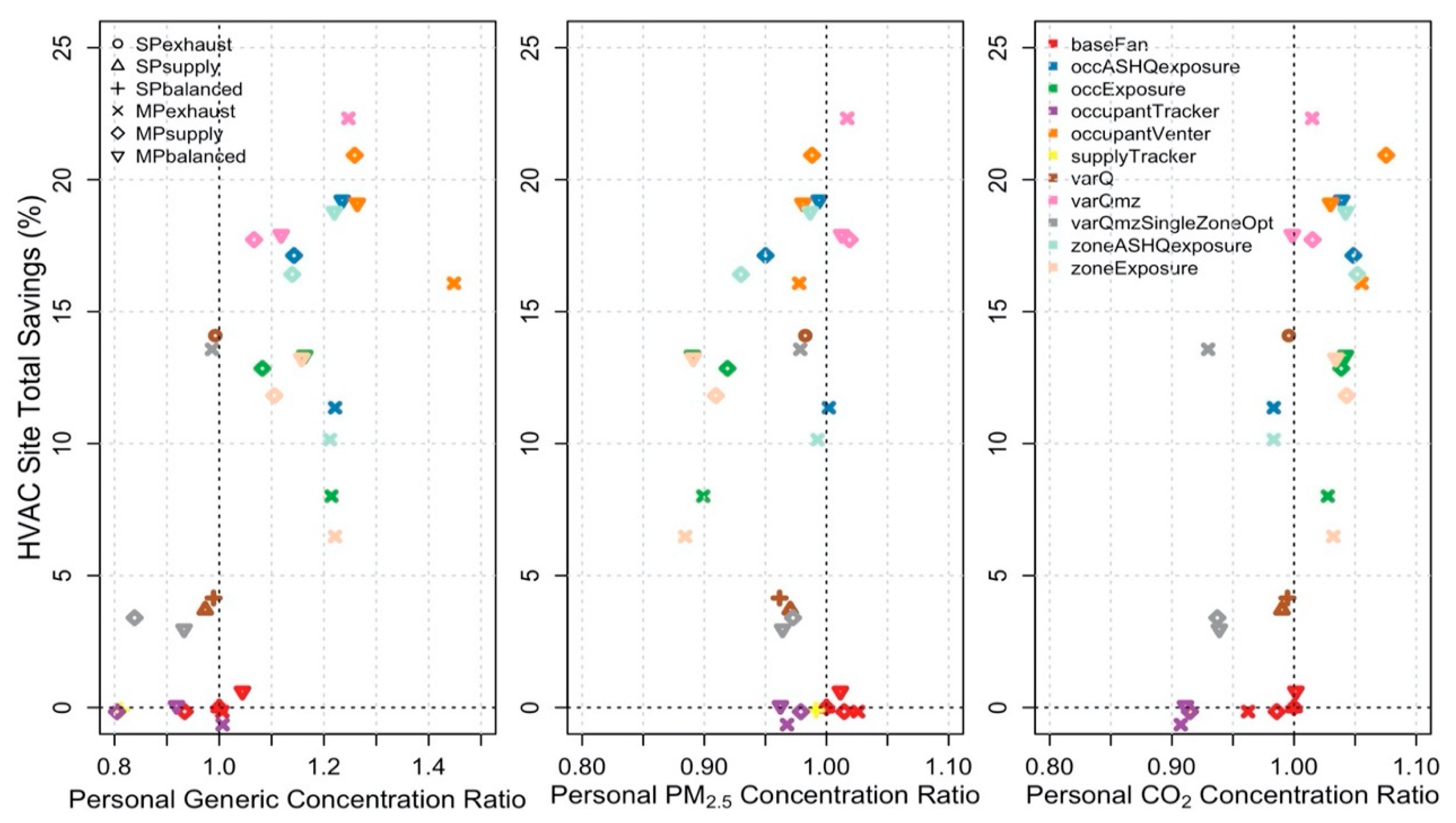
4.2. Summary of Ventilation Controls

Median personal concentrations, personal concentration ratios, energy savings, and air exchange rates are shown for each control type in

Table 4. Summary of median personal concentrations, personal concentration ratios, energy savings, and ventilation parameters for each ventilation control type.

Variable	Value	Personal Concentrations			Personal Concentration Ratios			Total HVAC Energy Savings		Ventilation Rate (h−1)	Reduction in Ventilation Rate (%)
		Generic (μg/m3)	PM2.5 (μg/m3)	CO2 (ppm)	Generic	PM2.5	CO2	kWh/m2	%
baseNoFan	Baseline	71.8	14.8	1481	3.75	1.24	1.83	2.66	36%	0.085	73%
baseFan	Baseline	20.9	12.3	783	1.00	1.00	1.00	0.00	0%	0.302	0%
occupantVenter	ZoneOcc	24.0	12.5	799	1.12	1.02	1.01	1.66	19%	0.279	30%
varQmz	Temp	27.5	12.4	836	1.30	0.99	1.06	1.83	18%	0.215	10%
occASHQexposure	ZoneOcc	24.7	12.2	797	1.18	0.99	1.03	1.64	17%	0.230	25%
zoneASHQexposure	ZoneOcc	24.4	11.9	798	1.17	0.97	1.03	1.51	15%	0.233	24%
occExposure	ZoneOcc	23.9	11.3	798	1.14	0.90	1.04	1.12	11%	0.251	18%
zoneExposure	ZoneOcc	24.0	11.2	802	1.15	0.90	1.04	1.04	11%	0.253	18%
varQ	Temp	21.1	11.7	788	0.98	0.97	0.99	0.60	7%	0.353	−14%
varQmzSingleZoneOpt	Temp	19.2	11.9	726	0.93	0.97	0.94	0.52	6%	0.354	−14%
supplyTracker	Tracker	15.6	11.9	706	0.81	0.99	0.91	−0.01	0%	0.322	0%
occupantTracker	Tracker	18.7	12.1	710	0.91	0.97	0.91	−0.03	0%	0.302	0%

. Humidity control (zone-hours >60% RH) and personal concentration hours that exceeded regulatory or design thresholds for CO₂ and PM_2.5 are shown for each controller in

Table 5. Median sum of personal- or zone-hours exceeding regulatory or design thresholds for each control strategy, including PM_2.5, CO₂, and relative humidity. PM_2.5 limits are based on 24-h threshold values from the U.S. EPA (35 μg/m³) and the World Health Organization (25 μg/m³). 5000 ppm CO2 is based on the OSHA Permissible Exposure Limit. 60% RH is a common design threshold for buildings.

Control Name	Control Category	24-h Mean PM2.5 > 35 μg/m3 (Personal Hours)	24-h Mean PM2.5 > 25 μg/m3 (Personal Hours)	CO2 > 5000 ppm (Zone Hours)	RH > 60% (Zone Hours)
baseNoFan	Baseline	11	13	0	6444
baseFan	Baseline	8	12	0	294
occupantVenter	ZoneOcc	9	12	0	367
varQmz	Temp	11	13	0	345
occASHQexposure	ZoneOcc	9	12	0	375
zoneASHQexposure	ZoneOcc	9	12	0	355
occExposure	ZoneOcc	8	12	0	338
zoneExposure	ZoneOcc	8	12	0	335
varQ	Temp	10	13	0	335
varQmzSingleZoneOpt	Temp	10	13	0	341
supplyTracker	Tracker	8	13	0	248
occupantTracker	Tracker	8	12	0	309

. The tables are sorted according to the total HVAC energy savings from largest to smallest. The total HVAC site energy savings and the personal concentration ratios for each contaminant are averaged and plotted by ventilation control type (color) and ventilation fan type (plot symbol) in Figure 4. Each control case is compared against the baseline constant fan case using the exact same fan type and configuration. For example, smart controls operating a multi-point supply fan are compared against the multi-point supply fan baseline case.

Whole dwelling average HVAC savings for the smart controls varied from 0% to 19%, and ventilation energy savings varied from 0% to 41%. Most zoned systems saved more HVAC energy than the unzoned, varQ, controller. Most control types reduced PM_2.5 concentrations (−10% to −1%), while most increased generic (+12% to +30%) and CO₂ (+1% to +6%) concentrations, and increased zone-hours exceeding 60% RH. This shows that there is a consistent tradeoff between increased/decreased personal concentration ratios for different contaminants. Controls that saved energy by reducing outside airflow achieved typical reductions in ventilation-related energy of 10% to 30%, compared to the 7% savings from the unzoned control (varQ). These savings were generally achieved at the expense of increased (i.e., worsened) personal concentrations, as well as increased zone-hours exceeding 60% RH. The Tracker controls did not save energy, instead they directed the same baseline dwelling airflows to occupied zones in an effort to reduce personal concentration ratios. These controls were successful at reducing personal CO₂ and generic concentrations (−9% to −19%), while PM_2.5 concentrations were only slightly reduced through smart control (−1% to −3%). Occupancy-based controls (ZoneOcc) had the strongest impacts of personal generic concentrations, mostly due to occupants entering previously unvented zones where the generic contaminant had accumulated during vacant periods.

Savings for heating generally made up the majority of total savings for most controls, with a median of 58% of total HVAC savings attributable to heating reductions (from 37% to 99%). The only control types with substantial cooling energy savings were varQ and varQmzSingleZoneOpt (11% of total HVAC savings). Occupancy-based controls marginally increased cooling energy use (<50 kWh annually). Air handler energy reductions typically made up small fractions of total savings, ranging from 2% to 7% of total HVAC savings. Ventilation fan energy was variable based on control type. For controls that reduced annual outside airflows, the reduction in ventilation fan energy typically made up 44–54% of total HVAC savings. In contrast, temperature-based controls that increased annual outside flows saw marginal increases in fan energy (median of 70 kWh).

Four control types were notable for having more modest impacts on personal concentrations, while reducing total HVAC energy use by 6 to 11%: occExposure, zoneExposure, varQ, and varQmzSingleZoneOpt. varQmzSingleZoneOpt is notable, because it used the same ventilation flows as the varQ control at each time-step (with 6–7% savings), but it directed those flows to occupied zones, which reduced Generic and CO₂ concentrations (−5%), but did not affect PM_2.5. While modest, these changes ensure that nearly every single case (i.e., all prototypes, climate regions, and envelope leakage rates) for this control had personal concentration ratios < 1, suggesting consistently improved IAQ by adding occupancy sensing and multi-point fans to this temperature-based control. The occExposure and zoneExposure controls are notable for large reductions in personal PM_2.5 concentrations (−10%). If reducing PM_2.5 concentrations is more important from a health perspective than increases in generic contaminants or CO₂, then these controllers offer significant energy savings (11%) with meaningful health benefits.

In general, all controls and baseline fan cases kept personal contaminant concentrations below regulatory or design thresholds for most hours of the year (see Table 5). Typically, there were fewer than 20-h per year where personal PM_2.5 concentrations exceeded either the WHO or EPA 24-h running average limits of 25 and 35 μg/m³. Changes associated with the smart controls were marginal relative to the baseline cases, adding only 1–3 h to the baseline exceedances. Personal CO₂ only exceeded 5000 ppm in a subset of non-ventilated (baseNoFan) apartment dwellings. In terms of zone-hours above 60% RH, the presence of any ventilation was by far the strongest impact, with the baseNoFan cases averaging 6444 zone-hours >60%, compared with at most 375 zone-hours for any of the control types. Compared with the baseline ventilation cases, all controls marginally increased zone hours > 60%, with the exception of the supplyTracker.

4.3. Variability of Results with the Simulation Parameters

Table 6. Median personal concentrations, concentration ratios, and energy savings aggregated by simulation parameters. Smart control cases only.

Variable	Value	Personal Concentrations			Personal Concentration Ratios			Total HVAC Energy Savings		Ventilation Rate (h−1)
		Generic (μg/m3)	PM2.5 (μg/m3)	CO2 (ppm)	Generic	PM2.5	CO2	kWh/m2	%
Prototype	1 story	24.1	11.5	783	1.154	0.963	1.036	1.17	14%	0.26
	2 story	24.8	11.9	787	1.096	0.966	0.998	1.38	12%	0.24
	apt	18.2	20.5	1093	1.214	0.974	1.050	−0.07	−1%	0.32
Fan Type	Exhaust	24.5	12.2	782	1.194	0.972	0.997	0.75	10%	0.26
	Supply	24.2	12.0	812	1.091	0.960	1.033	1.31	12%	0.24
	Balanced	22.8	11.6	784	1.143	0.962	1.012	1.42	14%	0.27
ACH50	0.6	24.4	11.4	789	1.160	0.952	1.020	1.28	13%	0.24
	2	24.5	11.7	788	1.128	0.965	1.014	1.30	13%	0.25
	3	22.1	12.9	802	1.115	0.973	1.014	0.77	9%	0.27
Climate Zone	1	22.9	11.7	786	1.129	0.968	1.022	1.15	11%	0.26
	3	23.1	11.9	785	1.139	0.965	1.021	0.81	13%	0.26
	10	24.3	12.1	795	1.137	0.964	1.013	0.72	11%	0.25
	16	24.7	12.5	812	1.115	0.965	1.010	1.95	11%	0.26
HVAC Mixed and Filtered MERV13	Yes	24.0	11.0	793	1.131	0.967	1.019	1.25	11%	0.26
	No	24.0	12.8	795	1.126	0.965	1.013	0.97	12%	0.26
Control Zones	2	23.0	12.0	786	1.105	0.973	1.005	0.96	10%	0.27
	4	24.4	11.8	804	1.174	0.944	1.036	1.33	14%	0.24

summarizes how the median personal concentrations, personal concentration ratios, ventilation rates and energy savings across all smart control types varied with the simulation parameters exercised in this study. Overall, the results were not very sensitive which indicates that any conclusions from this study can be applied to a large range of dwellings, locations, and ventilation systems. Some trends are discussed in greater detail below.

The greatest variability in the overall results was for apartments compared with single-family detached homes. In apartments, exposure to occupant-generated contaminants (PM_2.5 and CO₂) was substantially greater, despite higher ventilation rates in apartments (0.41 vs. 0.31 and 0.28 h⁻¹ in one- and two-story dwellings). Increased concentrations of PM_2.5 and CO₂ in apartments were due to greater occupant density in smaller volume spaces (27 m² per person in apartments versus 50 m² per person in one- and two-story dwellings), along with comparable indoor emissions of contaminants from cooking, dishwashing, and background sources. These changes in personal concentrations for apartments are likely the most impactful observed in this simulation study, in the sense that health-relevant differences are observed, most notably nearly double PM_2.5 concentrations (roughly 21 vs. 12 μg/m³). In addition, when personal concentrations were increased or decreased by controls, they were typically most changed in apartment dwellings. HVAC energy savings in apartments were negligible for controls that reduced annual ventilation rates, because decreases in ventilation also decreased the availability of ventilation cooling (i.e., economizing). These high-performance apartment buildings are cooling-dominated. In fact, adding mechanical baseline ventilation to the apartments reduced annual HVAC energy use by −501 kWh, while baseline ventilation increased energy use for one- and two-story homes by +527 and +868 kWh, respectively. This cooling energy use in apartments helped to control indoor humidity to lower levels compared with single-family dwellings, typically 43% in apartments, compared with 46–47% in two-story and 51% in one-story dwellings.

Ventilation fan type has major impacts on the ability to zonally ventilate, as well as on the energy and IAQ performance of baseline and smart control cases. Zoned exhaust fans effectively controlled CO₂ because of their ability to selectively ventilate bedrooms with closed doors during sleep hours. Exhausting directly from this higher concentration zone increased the local ventilation effectiveness (i.e., more contaminants are removed for a given quantity of air flow). Particle exposures were impacted negatively by zonal exhaust fans. Exhaust fans also have the lowest energy use. For control types that increased annual ventilation flows during mild weather periods (e.g., varQ), the small energy penalty of exhaust fan types ensured good energy performance for these outside-temperature-based controls (14% total HVAC savings for varQ using SPexhaust vs. 4% savings for other fan types). However, for controls that reduced annual ventilation flows (e.g., occExposure), the limited fan energy use also lessened the savings potential (8% total HVAC savings for occExposure using MPexhaust vs. 13% savings for other fan types). The whole dwelling ventilation rates and personal exposures provided by exhaust fans lies between supply and balanced fan types.

Supply fans reduced personal contaminant exposures for the generic contaminant and CO₂. As with exhaust fans, when the unzoned supply fan was located in the common zone of the home, it provided some protection from cooking contaminants, and when the supply flows were zoned, exposure to cooking contaminants worsened. The high fan energy required for supply fans made them use more energy than balanced systems but less than exhaust systems. They had the lowest dwelling ventilation rates. Paradoxically, because they used more energy, they could also save more energy when using smart controls that reduced annual outside airflow (e.g., zoneExposure). However, for the controls that used outdoor temperatures and increased annual outside airflows (e.g., varQ), they had poorer energy savings.

Balanced fans provided the highest dwelling ventilation rates, lowest exposures, and highest annual HVAC energy use. Yet, when comparing unzoned and zoned balanced systems, zoning increased personal exposure to the generic contaminant, and they very marginally worsened particle exposures, while improving CO₂. Balanced fans had the greatest ventilation energy savings for controls that reduced annual outside airflow.

This study focused on mechanically ventilated new dwellings that are not very leaky (0.6, 2, and 3 ACH₅₀). PM_2.5 was consistently elevated in cases with more envelope leakage, but the differences were typically moderate (<1 ug/m³ in most cases). Generic and CO₂ personal concentrations had substantial variability by envelope leakage, without a clear trend towards either increased or decreased concentrations. The leakiest three ACH₅₀ dwellings had marginally higher ventilation rates, which increased outdoor particles brought indoors. In smart control cases (see Table 6), Generic concentrations were lowest while PM_2.5 and CO₂ were highest in the three ACH₅₀ dwellings. Zonal controls in airtight cases were more impactful, because the zone airflows were fan-dominated, due to low infiltration rates. Whole dwelling HVAC energy savings from smart controls were also greatest in the 0.6 and 2 ACH₅₀ cases.

Baseline total HVAC energy use varied substantially by climate zone: 3 (1393 kWh), 10 (1611 kWh), 1 (2002 kWh), and 16 (3912 kWh). Yet, smart control savings percentages were similar across climate regions, with the greatest percent savings in CZ3. Climate zone had substantial impacts on personal contaminant concentrations, with CZ16 showing the highest average personal exposures for the generic contaminant, CO₂, and particles. CZ16 also had the highest average ventilation rate (0.307 vs. 0.299–0.300 h⁻¹). CZ16 consistently showed both the highest annual consumption (3912 kWh) and the greatest absolute energy savings from smart controls. For example, the best energy savings strategy (varQmz) saved 21% in CZ16 (880 kWh saved) but only 18% in CZ10 (266 kWh saved).

Two electric heat pump HVAC system types were assessed in this work: (1) a central recirculating ducted air handler system with MERV 13 supply air filter (Mixed and Filtered) that mixed air between zones when operating; and (2) a decentralized ductless system without filtration and no forced mixing between zones (not mixed and filtered). Despite inter-zone mixing with the mixed and filtered system, the only contaminants with substantial differences by HVAC type were particles, which were removed by the MERV 13 filter (+1.9 ug/m³ and +17% for baseline cases without MERV 13). On average, the mixed and filtered cases used more energy (+450 kWh per year) due to the recirculating fan energy, but percent energy savings for smart controls were very similar.

One question that arises is: how many zones are enough to capture zoning effects? In order to assess this, we examined two zoning configurations for several of the zonal controls. In addition to the cases already discussed where the homes were split into four or more zones, we performed additional simulations and analysis with the homes split into only two zones. The two zones were all of the bedrooms grouped into one zone and all the other rooms grouped into another zone. Figure 5 shows annual median values of personal concentrations compared between these zoning configurations. For almost all cases the differences are small, a few percent or less, indicating that the extra complexity and expense of more zones is not justified. The exception is the occupantVenter control that has significant advantages for generic and CO₂ exposure if only two zones are controlled. Figure 6 shows the energy use changes when extra control zones are used. It is clear that the occupantVenter strategy increased energy savings with additional zones, but this was done at the expense of increased personal concentrations. For the apartment, these results show that smart controls actually increase annual HVAC energy use (negative savings).

5. Conclusions

Controls that saved energy by reducing outside airflow achieved typical reductions in ventilation-related energy of 10% to 30%, compared to the 7% savings from the unzoned control (varQ). Most zone controls saved energy by reducing outside ventilation airflow. However, this was often accompanied by a tradeoff with increased personal concentrations for some contaminant types. The added complexity of including extra control zones beyond a sleeping/non-sleeping split is not justified, due to modest energy savings and usually increased concentrations. On average, the varQ, varQmzSingleZoneOpt, supplyTracker, and occupantTracker controls maintained personal concentrations for all contaminants that were less than those for the constant flow baseline cases, though individual cases increased personal concentrations relative to the baseline. Of these four controls, only the varQ versions saved energy, the Tracker controls were solely designed to improve IAQ by directing ventilation flows to occupied spaces. The occExposure and zoneExposure controls were notable for reducing total HVAC energy by 11% on average, while reducing PM_2.5 personal concentrations by 10%. However, they substantially increased generic and CO₂ concentrations. Future work should investigate metrics that combine the health impacts of different contaminants, so that trade-offs between contaminants can be made. Multi-family dwellings showed reduced energy savings (and were most often negative), because they are cooling-dominated, and reducing ventilation rates through zone occupancy control reduced free ventilation cooling. Advanced economizing strategies are likely more promising in such dwellings.

Exhaust fans used the least energy, but they were only effective as zonal systems when large differences in zone concentrations existed (e.g., CO₂ in bedrooms with doors closed at nighttime, or on the second level of a two-story dwelling). Supply ventilation types (including balanced fans) most effectively delivered outside air to the target zones, but they also used much more energy than exhaust systems, due to their recirculation and tempering requirements. Balanced fan types had the highest ventilation rates, but also the highest energy use of all fans assessed.

Relative to single-point, unzoned ventilation systems, zoning was found to have small effects (<5%) on personal pollutant concentrations in the majority of cases. Zonal ventilation was most impactful when unzoned systems did not evenly serve the dwelling. An example includes two-story dwellings, where pressure interactions with the building envelope meant the first and second levels were ventilated at substantially different rates by unzoned supply and exhaust fans located in the common zone. Zonal ventilation was also impactful when patterns of point-source contaminant emissions (e.g., cooking, breathing, bathing) inadvertently were aligned (or not aligned) with the location of the single-point fan. For example, we observed benefits for unzoned ventilation systems that were located in the kitchen, where cooking contaminants were emitted. In contrast, zoned ventilation systems reduced CO₂ in bedrooms with closed doors. These results suggest that the supply or exhausts of a zoned system may be best located in bedrooms and kitchen areas, where contaminants are emitted and where occupants spend substantial uninterrupted periods of time.

References

1. Guyot, G.; Sherman, M.H.; Walker, I.S. Smart Ventilation Energy and Indoor Air Quality Performance in Residential Buildings: A Review. Energy Build. 2018, 165, 416–430. [Google Scholar] [CrossRef] [Green Version]
2. Sherman, M.H.; Walker, I.S. Meeting Residential Ventilation Standards through Dynamic Control of Ventilation Systems. Energy Build. 2011, 43, 1904–1912. [Google Scholar] [CrossRef] [Green Version]
3. Sherman, M.H.; Walker, I.S.; Logue, J.M. Equivalence in Ventilation and Indoor Air Quality. HVACR Res. 2012, 18, 760–773. [Google Scholar] [CrossRef]
4. Less, B.D.; Dutton, S.M.; Walker, I.S.; Sherman, M.H.; Clark, J.D. Energy Savings with Outdoor Temperature-Based Smart Ventilation Control Strategies in Advanced California Homes. Energy Build. 2019, 194, 317–327. [Google Scholar] [CrossRef] [Green Version]
5. Lubliner, M. Energy Savings Potential of Controlling Residential Whole-House Ventilation System Operation Based on Outside Temperature. In Proceedings of the Environmental Health in Low Energy Buildings, Vancouver, BC, Canada, 15–18 October 2013; ASHRAE: Vancouver, BC, Canada, 2013; pp. 215–221. [Google Scholar]
6. Walker, I.S.; Sherman, M.; Dickerhoff, D. Development of a Residential Integrated Ventilation Controller; Lawrence Berkeley National Laboratory: Berkeley, CA, USA, 2012. [Google Scholar]
7. Less, B.; Walker, I.S.; Tang, Y. Development of an Outdoor Temperature-Based Control. Algorithm for Residential Mechanical Ventilation Control; Lawrence Berkeley National Laboratory: Berkeley, CA, USA, 2014. [Google Scholar]
8. Less, B.; Walker, I.S.; Ticci, S. Development of Smart Ventilation Control Algorithms for Humidity Control in High-Performance Homes in Humid U.S. Climates; Lawrence Berkeley National Laboratory: Berkeley, CA, USA, 2016. [Google Scholar]
9. Less, B.; Walker, I.S. Smart Ventilation Controls for Occupancy and Auxiliary Fan Use across U.S. Climates; Lawrence Berkeley National Laboratory: Berkeley, CA, USA, 2017. [Google Scholar]
10. Clark, J.D.; Less, B.D.; Dutton, S.M.; Walker, I.S.; Sherman, M.H. Efficacy of Occupancy-Based Smart Ventilation Control Strategies in Energy-Efficient Homes in the United States. Build. Environ. 2019, 156, 253–267. [Google Scholar] [CrossRef] [Green Version]
11. Martin, E.; Fenaughty, K.; Parker, D. Field and Laboratory Testing of Approaches to Smart Whole-House Mechanical Ventilation Control; National Renewable Energy Laboratory: Golden, CO, USA, 2018. [Google Scholar]
12. Turner, W.J.N.; Walker, I.S. Using a Ventilation Controller to Optimise Residential Passive Ventilation for Energy and Indoor Air Quality. Build. Environ. 2013, 70, 20–30. [Google Scholar] [CrossRef]
13. Young, M.; Less, B.D.; Dutton, S.M.; Walker, I.S.; Sherman, M.H.; Clark, J.D. Assessment of Peak Power Demand Reduction Available via Modulation of Building Ventilation Systems. Energy Build. 2020, 214, 109867. [Google Scholar] [CrossRef]
14. Less, B.; Walker, I.; Lorenzetti, D.; Mills, E.; Rapp, V.; Dutton, S.; Sohn, M.; Li, X.; Clark, J.; Sherman, M.; et al. Smart Ventilation for Advanced California Homes; LBNL-2001342; 2020. Available online: https://www.osti.gov/biblio/1635274/ (accessed on 1 June 2020).
15. Offermann, F.J. Ventilation and Indoor Air Quality in New Homes; California Energy Commission and California Air Resources Board: Sacramento, CA, USA, 2009. [Google Scholar]
16. Hult, E.L.; Willem, H.; Price, P.N.; Hotchi, T.; Russell, M.L.; Singer, B.C. Formaldehyde and Acetaldehyde Exposure Mitigation in US Residences: In-Home Measurements of Ventilation Control and Source Control. Indoor Air 2015, 25, 523–535. [Google Scholar] [CrossRef] [PubMed] [Green Version]
17. Persily, A. A Modeling Study of Ventilation, IAQ and Energy Impacts of Residential Mechanical Ventilation; National Institute of Standards and Technology: Gaithersburg, MD, USA, 1998. [Google Scholar]
18. Emmerich, S.; Howard-Reed, C.; Gupte, A. Modeling the IAQ Impact of HH1 Interventions in Inner-City Housing; National Institute of Standards and Technology: Gaithersburg, MD, USA, 2005. [Google Scholar]
19. California Energy Commission. Alternative Calculation Method Approval Manual for the 2019 Building Energy Efficiency Standards—Title 24, Part. 6, and Associated Administrative Regulaions in Part. 1; California Energy Commission: Sacramento, CA, USA, 2018. [Google Scholar]
20. Emrath, P. Berkeley Spaces in New Homes; National Association of Home Builders: Washington, DC, USA, 2013. [Google Scholar]
21. ASHRAE Standard 62.2. Ventilation and Acceptable Indoor Air Quality in Residential Buildings; American Society of Heating Refrigeration and Airconditioning Engineers: Atlanta, GA, USA, 2019. [Google Scholar]
22. HVI. Certified Home Ventilating Products Directory; Home Ventilating Institute: Cheyenne, WY, USA, 2019. [Google Scholar]
23. Kim, S.; Walker, I.; Delp, W. Development of a Standard Test. Method for Reducing the Uncertainties in Measuring the Capture Efficiency of Range Hoods; Lawrence Berkeley National Laboratory: Berkeley, CA, USA, 2017; p. 39. [Google Scholar]
24. ASHRAE Standard 160. Criteria for Moisture Control Design Analysis in Buildings; American Society of Heating Refrigeration and Airconditioning Engineers: Atlanta, GA, USA, 2016. [Google Scholar]
25. Woods, J.; Winkler, J. Effective Moisture Penetration Depth Model for Residential Buildings: Sensitivity Analysis and Guidance on Model Inputs. Energy Build. 2018, 165, 216–232. [Google Scholar] [CrossRef]
26. Woods, J.; Winkler, J.; Christensen, D. Moisture Modeling: Effective Moisture Penetration Depth versus Effective Capacitance. In Proceedings of the Thermal Performance of Exterior Envelopes of Whole Buildings XII; ASHRAE/DOE/BTECC: Clearwater Beach, FL, USA; American Society of Heating Refrigeration and Airconditioning Engineers: Atlanta, GA, USA, 2013. [Google Scholar]
27. Chan, W.R.; Kim, Y.-S.; Less, B.D.; Singer, B.C.; Walker, I.S. Ventilation and Indoor Air Quality in New California Homes with Gas. Appliances and Mechanical Ventilation; LBNL-2001200; Lwrence Berkeley National Laboratory: Berkeley, CA, USA, 2019. [Google Scholar] [CrossRef]
Figure 1. Example controller flowchart for the zoneExposure controller. This control process is for a single zone and is repeated for each zone in the dwelling. “RE” is the relative exposure calculated for an individual zone.
Energies 14 05257 g001
Figure 2. Comparison of baseline personal exposures for single– and multi–point configurations. Fan types include exhaust (left), supply (middle) and balanced (right) for a 24 h period for an individual occupant not in the dwelling from 9 a.m. to 5 p.m. and moving between zones.
Energies 14 05257 g002
Figure 3. Differences in personal concentrations when a controlling a multi–point supply fan using the occExposure control strategy following a single occupant for 24 h who is absent from the dwelling from 9 a.m. to 5 p.m. and moving between zones during waking hours. Positive values indicate that occExposure increased personal concentrations compared with the constant multi–point supply fan baseline.
Energies 14 05257 g003
Figure 4. Annual median total HVAC site energy savings (%) and personal concentration ratios for each contaminant, control type, and fan type.
Energies 14 05257 g004
Figure 5. Comparison of annual median personal contaminant exposure by for systems controlling all zones or only two zones for different control strategies (colours) and dwelling types (symbols).
Energies 14 05257 g005
Figure 6. Comparison of energy use for systems controlling all zones or only two zones for different control strategies (colours) and dwelling types (symbols).
Energies 14 05257 g006