Article

Economic and Carbon Costs of Electricity Balancing Services: The Need for Secure Flexible Low-Carbon Generation

1
Centre for Environment and Sustainability, University of Surrey, Guildford GU2 7XH, UK
2
Thames Water Utilities Ltd., Reading RG1 8DB, UK
3
Department of Chemical and Process Engineering, University of Surrey, Guildford GU2 7XH, UK
4
Department of Civil and Environmental Engineering, University of Surrey, Guildford GU2 7XH, UK
*
Author to whom correspondence should be addressed.
Energies 2021, 14(16), 5123; https://doi.org/10.3390/en14165123
Submission received: 15 May 2021 / Revised: 27 July 2021 / Accepted: 11 August 2021 / Published: 19 August 2021
(This article belongs to the Special Issue Energy Policy and Policy Implications 2020)

Abstract

:
The electricity sector aims to achieve a balanced progress in all three dimensions of the energy trilemma: affordability, decarbonisation and security of supply. Separate strategies for decarbonisation and security of supply have been pursued; each with close attention to minimising costs, thus consistent with the affordability aspect of the trilemma. However, while it is evident that the pathway for decarbonisation increases pressure on security of supply, the pressures that cost-minimising security of supply measures are putting on decarbonisation goes unaddressed. The United Kingdom (UK) is a global leader in the transition towards a decarbonised economy and aims to achieve net-zero emissions by 2050. As a major part of the UK, Great Britain (GB) has achieved greater than 50% of low-carbon electricity generation and the grid’s carbon intensity has dropped by 36% over the period 2015–2019. However, balancing services that provide security of supply uses only 8% of low-carbon generation. Their carbon intensity is double the grid’s average and this gap is widening. This is an effect of a systemic reliance on carbon-intensive fuels. Financial support for capital investment for flexible low-carbon technologies is much needed. The GB context suggests that an integrated strategy covering all three dimensions of the trilemma might achieve an improved balance between them and unlock an affordable, net-zero emissions and secure power system.

1. Introduction

National energy systems are facing unprecedented challenge for change as key components of the global efforts towards sustainability. Sustainable development, as the management of economic, environmental and social aspects, such that the current generation’s action does not inhibit the ability of future generations to meet their needs, is fundamental to achieving global prosperity [1]. In fact, concerted and balanced actions to achieve economic, environmental and social sustainability are required [2]. These three pillars of sustainability apply to all the energy sectors as the dimensions of the well-known “energy trilemma”: providing equitable, clean and adequate energy [3,4]. The aim of sustainable development in the energy sectors, and more specifically in the electricity sector, is therefore to progress towards a balanced system that reflects all three dimensions of the Trilemma.
This article adopts the terminology for the Trilemma as it is generally understood in the electricity sector: affordability, decarbonisation and security of electricity supply (SoES):
  • Affordability is the main parameter to measure economic accessibility to electricity, in particular for vulnerable users [4,5].
  • Decarbonisation aims to reduce greenhouse gas (GHG) emissions, typically measured in the equivalent impact of carbon dioxide emissions (CO2eq), ultimately seeking net-zero emission power systems [4].
  • SoES is defined as “the ability of an electricity system to supply final customers with electricity” [6]. In general, this dimension aims to achieve a resilient system composed by a diverse fuel mix [4] that can reliably fulfil current and future demand [7].
The current challenge in the electricity sector is to deliver a secure and fully decarbonised power system at the lowest possible cost [8,9] and the careful integration of these three dimensions to unlock the potential for a sustainable power system. However, these three dimensions are generally considered mutually competitive and, in this sense, are understood as a Trilemma.
In the last decades, policies to support the decarbonisation of the electricity grid have been set in many countries. The main driver is that electricity generation is a major source of GHG emissions and thus one of the main contributors to climate change [10]. These policies typically focus on incentivising the installation of capacity of low-carbon technologies (LCTs), or the subset of renewable electricity sources (RES).
However, this desired increase of electricity generated from RES often results in lower SoES [11,12,13,14]. This is because the most widely installed generation technologies for renewable electricity (wind and solar photovoltaic) are weather-dependent and, in the case of photovoltaic, also time of day dependent. Therefore, their generation varies in space and time, exacerbating the problem of matching supply with the variable demand. It is clear that intermittent RES alone are not able to match the variable demand and other technologies are needed to secure the balancing of demand and supply [15,16,17,18]. Thus, markets and policies are designed to ensure SoES by means of real-time balancing services and on-demand capacity services.
SoES is achieved by ensuring enough power is generated to balance the demand in real time, with appropriate reserve. In general, the two main approaches for balancing the grid are by aggregating over space and/or averaging over time:
  • Aggregation over space is achieved by combining different technologies or interconnectors between areas [11,19,20]. Currently, interconnectors and the integration of fossil-fuelled thermal power units into the generation mix, alongside renewables, generally provide SoES [21,22,23].
  • Alternatively, a power system is balanced by averaging demand or supply over time. Electricity storage systems are examples of averaging supply over time [24,25,26], while demand side response (DSR) is an approach of managing demand over time [27].
Balancing is traditionally provided by fossil-fuelled generation [14], which can provide “firm” power, and is typically flexible and hence dispatchable. Few studies have investigated the feasibility and effects of using, among the RES, bioenergy sources to support balancing the grid [28,29,30]. These studies found that current limitations include increased capital investment and reduced operational efficiency of the generation plants. This is because of the reduced and non-optimal generation plant loading during extensive off-peak times; however, the use of RES in balancing was expected by these authors to be beneficial in both economic and environmental dimensions in the long term.
Flexible low-carbon generation could in principle be provided by several technologies that currently are not fully exploited or have not traditionally bid into these markets. Concentrating solar, hydro and bioenergy power stations are existing technologies and fuels suitable to provide flexible generation [13,31]. Hydro, and pumped hydro storage (PHS), are largely used for flexible generation. Bioenergy (in solid, liquid or gaseous forms) can be produced, stored and used according to the demand at peak time [29,32,33,34,35].
This work aims to assess the need for renewable flexible generators within the services designed to balance demand and supply in real time. The balancing services constitute a real-time subsector of the electricity sector, the economic, environmental and social impacts of which are not assessed in the academic literature. Whilst many authors focus on the benefits and viability of different approaches [36,37] or the contribution of specific technologies [38,39,40] to provide SoES, a comprehensive investigation of the balancing services is lacking (e.g., [8,41,42]). In fact, the analysis of economic and environmental costs of balancing services in a highly decarbonised electricity system has not been attempted yet in the literature. After examining the status of the balancing services and highlighting the diverging development pathways occurring whilst trying separately to decarbonize the system and securing electricity supply, this article identifies areas of improvement of current policies.
This article uses the highly decarbonised system of Great Britain (GB) as a case study [43]. GB is a single area where markets and balancing services operate, and energy policies apply. In GB, security of electricity supply is provided by several services to ensure real-time balance between demand and supply, with adequate reserve [44]. The main services, investigated in this article, are the capacity market (CM) and the balancing mechanism (BM).
This analysis is timely as the UK government has recently legislated to commit the country to the ambitious target of net-zero carbon emissions by 2050. The Committee on Climate Change (CCC) [45] suggests that to achieve this target, major, well-designed and urgent policies and actions are required, particularly in hard to decarbonise sectors. To achieve this target, a 68% reduction of GHG emissions 1990s levels by 2030 is recommended [46]. All industrialized economies face similar challenges, and thus the article’s findings for GB have wider international relevance. In this context, this article aims to contribute towards the definition of strategies that will ultimately lead to the development of the net-zero power system.

2. Materials and Methods

This article analyses the economic costs and carbon impacts of SoES by analysing the two main balancing services in GB: the BM and the CM.
The CM allows National Grid Electricity System Operator (NG-ESO) to buy dispatchable capacity in advance at a fixed price. The cost is set by competitive award of contracts through technology neutral auctions. The cost is therefore expected to be the lowest possible, as competition promotes affordability. Auctions for securing dispatchable capacity take place one and four years ahead of delivery (defined respectively as T-1 and T-4). Close to the beginning of a settlement period (SP), the half-hourly period in which the grid operates, if forward trading shows risk of imbalances, NG-ESO can instruct contracted capacity providers to supply dispatchable power (if generators) or to reduce use (if DSR providers) [47].
In contrast, the BM operates on a near real-time basis: up to 5 min before the beginning of a SP, generators and users are instructed to increase or reduce generation according to their “offers” (in case of making more power available) and “bids” (in case of reducing generation) [48]. Offers and bids are placed by operators and accepted by the system operator according to the volume needed. In both cases, flexibility in operations is needed. When more power is needed, operators need to be able to flexibly increase generation as required. Therefore, on-demand energy availability is essential. This condition is a limitation on the use of many LCTs in the BM and constitutes a constraint for the system.
The electricity system regulator, OFGEM [49], modified the methodology to calculate the BM price (price average reference—PAR). Until 5 November 2015, the final price was calculated as the average price of the marginal 500 MW traded on the BM (called PAR500). After that date, the marginal 50 MW set the price (PAR50). Since 1 November 2018, the price has been calculated as the average price of the marginal 1 MW traded on the BM (PAR1). To ensure internal consistency of the market conditions of the period studied, the PAR50 period is used for the economic analysis presented in this work.
The method for the analysis of the economic and carbon costs of the balancing services is detailed below. While the method for the assessment of the economic costs is developed specifically for this work, the carbon costs assessment method improves on existing datasets by adopting a consistent approach for the estimation of carbon factors of each electricity source based on the data available. As such, the description of the method and the data used is presented together in this section.
The yearly economic costs (Equation (1)) are assessed by summing all the 17,520 annual half-hourly (hh) generation and pricing data for the BM (Equation (2)) and the yearly results of capacity auctions for the CM (Equation (3)). Then, the results are compared to the overall electricity cost to consumers and market price values, in order to assess the effects of SoES on affordability.
T o t a l   c o s t s y e a r = C o s t s B M , y e a r + C o s t s C M , y e a r
in which
C o s t s B M , y e a r = h h = 1 17520 M a r k e t   p r i c e h h × V o l u m e   t r a d e d h h
and
C o s t s C M , y e a r = T - 4   a u c t i o n   c o s t s y e a r + T - 1   a u c t i o n   c o s t s y e a r
Affordability is commonly assessed by comparing the average total net annual cost of energy (in all forms) per domestic consumer with the median annual household disposable income. The threshold of considering a system affordable is generally when this ratio is below 10% [50,51]. For this purpose, electricity is assumed to represent half of the total energy costs for a household (based on [52]). However, whilst this methodology measures the average affordability of an energy system, in practice the issue of households’ energy affordability impacts mainly those on low incomes. In fact, the proportion of total expenditure on energy in low-income households is double the average [53].
Data were collected from the system operator and the administrators of the balancing services. The analysis of the BM is based on the derived BM unit data available by accessing the Elexon database through application programming interfaces [54]. Statistics of accepted offers and bids from all generating units can be published for each half hour. By matching each unit with their fuel based on Elexon [55] and other databases [56,57], generation per fuel in each half hour was calculated during the whole PAR50 period. Data for the capacity market are available from National Grid [56,57,58,59,60].
The carbon impacts are calculated in terms of overall carbon intensity (CI). The CI measures GHG emissions as total amount of CO2 equivalent (CO2eq) emissions per unit of electricity, i.e., gCO2eq/kW·h.
The calculation of carbon impact of the marginal electricity generation is not new. Several authors calculate the marginal emission factors (MEF) by statistically analysing the hourly or half-hourly variation in load and fuel mix of the grid as a whole (e.g., [61,62,63,64,65,66]). Whilst the established statistical methods for the calculation of the MEF are an effective indirect proxy, this article directly analyses the data of balancing services. The statistical calculation of the MEF using data from the grid as a whole [61] assumes as marginal any variation in power generation from a period to the following, irrespective of whether it was in fact due to balancing purposes. If looking at data of the grid as a whole, the increase or decrease in power generation and the variation in fuel mix is due to multiple factors and it is not related only to balancing services. However, the focus of the work presented in this article is the assessment of the impacts of SoES and, hence, of the balancing services.
In this work the empirical data of only the power traded near to real time under the balancing services for the achievement of SoES is analysed (i.e., the marginal short-term balancing power generation). In particular, the method described below allows identification and includes only the actual marginal power generated and traded on the near real-time markets for balancing purposes. The choice of this method is made to unequivocally identify the variation in generation and fuel mix due to and traded for ensuring SoES. The BM and CM are de facto assumed to be two separate subsectors of the electricity supply system, and the method calculates the emissions associated with them.
Emissions from the BM are calculated by multiplying CIs and generation data for each fuel (f) and technology (t) in each half hour (hh). The overall CI is then calculated by dividing the total emissions by the total generation traded on the BM (Equation (4)).
C I B M , y e a r = h h = 1 17520 f = 1 n C I t , f , h h × G e n e r a t i o n t , f , h h T o t a l   G e n e r a t i o n y e a r  
Similarly, the annual CI of the CM is calculated by multiplying the generation and the CI for each fuel (Equation (5)). For the purpose of this work, the total generation of the CM is calculated assuming that the capacity secured is equally used for generation during the peak hours (16:00–20:00) [34,35] of the winter period (November–March), which is the period of higher stress for the grid [67].
C I C M , y e a r = f = 1 n C I t , f × G e n e r a t i o n f T o t a l   G e n e r a t i o n y e a r  
One of the contributions to knowledge of this article is the development of new consistent reference values for CIs per fuel and technology. Whilst some reference values for CIs per fuel exist in the literature [68,69,70], they use an inconsistent methodology for the different fuels. Additionally, the CIs database needs to be updated to provide new references for the more detailed generation by fuel data reporting.
In this work, CIs per fuel are calculated over the period 2014–2020 based on generation statistics from BEIS [71,72] and carbon emissions reported by BEIS and DEFRA [73,74,75,76,77,78].
The calculation of CIs for generation from bioenergy sources (“other”, in the GB generation statistics) and PHS is particularly relevant for the purpose of this article. The category of “other” renewables includes generation from various bioenergy sources: biogas from anaerobic digestion of organic waste, biodegradable waste and vegetable and animal biomass. Staffell [68] discussed the complexity of calculating CI for these “other” renewable sources and biomass in particular. The current common approach for the calculation of GHG emissions from these sources includes CH4 and N2O emissions from the scope-1 direct use of the fuel (ignoring direct CO2 emissions) plus all lifecycle GHG emissions along the supply chain due to extraction, refining and transportation of bioenergy sources (scope-3) [79,80,81]. The rationale for this approach is that direct CO2 emissions are considered outside of scope, being balanced by the emissions absorbed by bioenergy sources during their growth [81], on the assumption that the bioenergy is grown sustainably, with appropriate replanting. On the contrary, the emissions for fossil fuels are normally calculated following the consumption-based accounting methodology and therefore include only the scope-1 emissions, notwithstanding that scope-3 emissions represent a non-negligible amount [68]. Using different methodologies for fossil fuels and renewables leads to inconsistencies in the datasets available in the literature, which makes the comparisons of the emissions associated with different fuel mixes problematic.
As an important first step, a consistent dataset of reference values for the CI for each fuel is developed based on scope-1 for all fuels. This will allow comparisons of the emissions associated with different fuel-mix scenarios for balancing services. The new dataset should be consistent with results for fossil-fuelled generation in existing literature sources, but the calculated CIs for the “other” bioenergy sources will be lower when compared to the existing sources, as these include scope-3. As in the future scope-3 emissions for all fuels will become more significant, Appendix A shows the CIs if recalculated consistently for all fuels to include these emissions.
As CIs calculated in this article are intended for the calculation of emissions of total positive net generation, CIs for each generating technology are calculated as the total carbon factor (CF) arising from the use of each specific fuel (f) divided by the typical efficiency of the generation technologies (t) using each fuel (Equation (6)). As the efficiency is intended to be net of plant self-consumption, it is calculated for each fuel by dividing gross energy consumption by electricity supplied (Equation (7)).
C I t , f = C a r b o n   F a c t o r f E f f i c i e n c y t , f
in which
E f f i c i e n c y t , f = G r o s s   e n e r g y   c o n s u m p t i o n t , f E l e c t r i c i t y   s u p p l i e d t , f  
The calculations included in this article provide a more consistent accounting of emissions. Additionally, the figures detail or update previous GB-specific assessments by Staffell [68], Bruce et al. [69] for NG-ESO and Rogers and Parson [70]. In effect, until November 2017, all bioenergy sources were included in one single “other” category in GB statistics. Staffell [68] calculated CI for this category by assuming it is entirely constituted by biomass; however, in reality it included all bioenergy sources. In fact, Elexon now reports separate generation statistics for biomass and the remaining bioenergy sources.
The development of a methodology for the calculation of CIs for biomass and the “other” renewables constitutes a novel contribution of this work.
CIs for biomass and the “other” bioenergy sources are estimated as presented in Equation (8) as weighted average of the number (n) of fuels (f). The CI is calculated by weighting the CFs from bioenergy fuels published by BEIS and DEFRA [73,74,75,76,77,78] according to their relative contribution to the final generation of the category. Table 6.4 of the energy statistics published by BEIS [72] provides statistics of generation from all sources of bioenergy.
C I t h e r m a l   r e n e w a b l e s = f = 1 f = n C F f E f f i c i e n c y f × G e n e r a t i o n f f = 1 f = n G e n e r a t i o n f
Biomass and co-firing with fossil fuels are assumed to be all fuelled by wood pellets (since the largest biomass power plants are fuelled by such biomass [82]). The categories of anaerobic digestion, animal biomass, biodegradable energy from waste and sewage gas in BEIS [72] are assumed as biogas-fuelled in BEIS and DEFRA reporting data [73,74,75,76,77,78]. The last category of landfill gas only comprises generation from this fuel.
PHS is generally considered zero emissions as it is not a generation technology. However, carbon emissions are related to the electricity consumed and losses in the process. For the calculation of average grid CI, these carbon emissions are normally accounted only at generation, disregarding the losses. However, for the emissions from the BM, the specific CI for PHS is calculated as presented in Equation (9) for each half hour (hh) as the weighted average of the grid’s CI to actual use in the previous 18 h (36 half hours) and then divided by overall cycle efficiency, calculated as 72.5% [72].
C I P H S , h h = t = h h 1 t = h h 37 C I g r i d , t × C o n s u m p t i o n P H S , t t = h h 1 t = h h 37 C o n s u m p t i o n P H S , t E f f i c i e n c y P H S  
Emissions for French, Dutch and Irish imports or exports are included on consumption-based accounting, considering each country CI’s annual average [83,84,85].
Finally, as this methodology only accounts for scope-1 emissions, LCTs (wind, solar and nuclear) are assumed to be carbon neutral.

3. Results

As decarbonisation progresses at pace, preserving the SoES has become the immediate concern. Balancing and capacity services have been devised to ensure SoES. In this section, the economic and carbon impacts of SoES are measured.

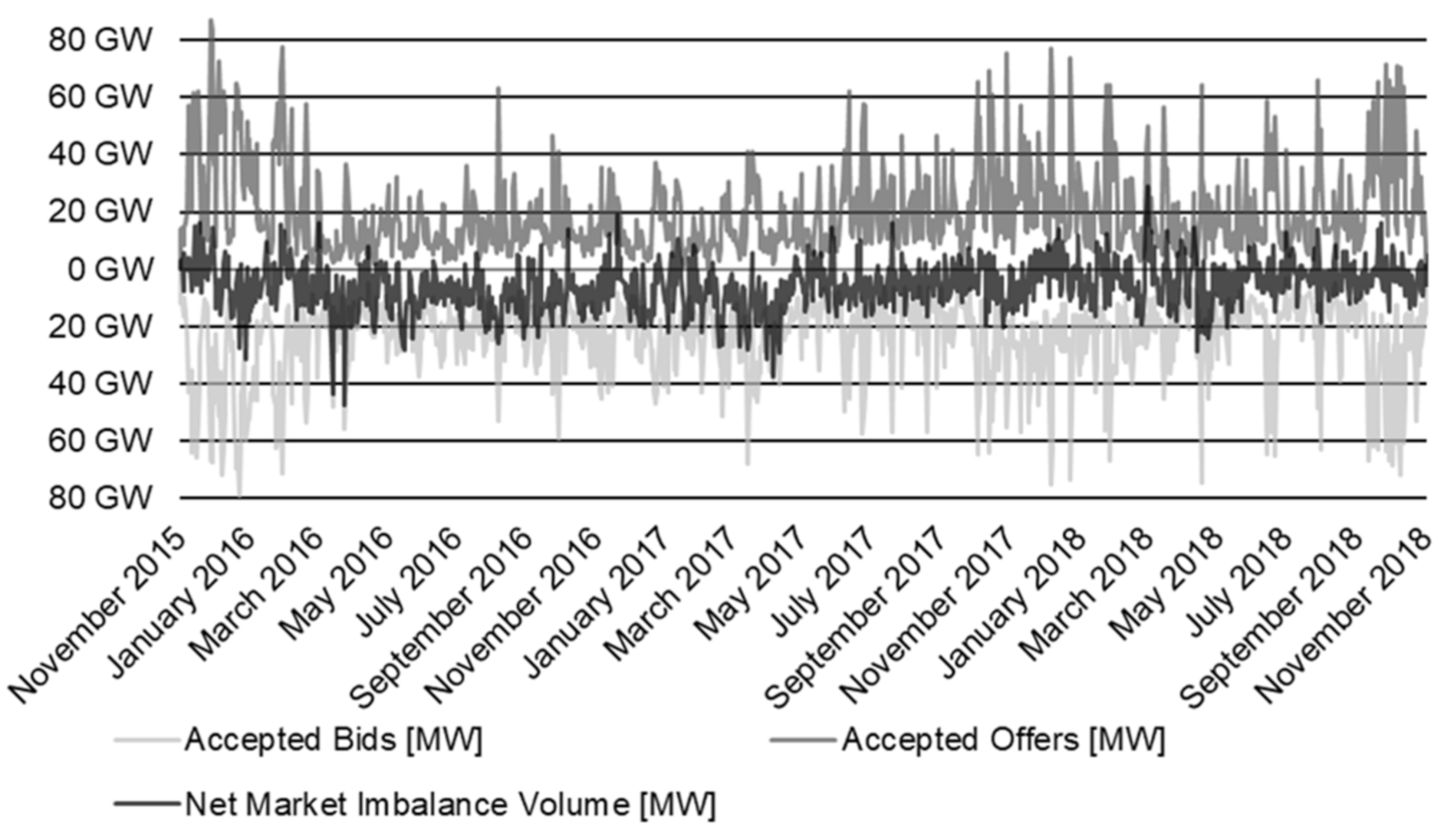
3.1. The Economic Cost of Balancing Services

The CM and other balancing services have prearranged prices to make capacity available when needed. CM volumes and costs awarded in recent auctions are reproduced in Table 1. The average of the initial three delivery years is an estimate of the yearly cost of security of supply provided by CM and is nearly GBP 1.0 billion.
On the contrary, the overall cost of BM depends on the traded volumes and market prices, which are variable on a half-hour basis according to several factors. The market price is determined according to the price required to activate the marginal capacity provider in each specific half hour, as presented in Section 2.
The evolution of the price calculation methodology has contributed to increasing average prices and, largely, higher market volatility. Figure 1 provides a graphical representation of trends of average daily real prices and spread. In particular, the evolution of the PAR calculation methodology has directly affected affordability by increasing prices and indirectly by increasing the operational risk of electricity suppliers by developing a more volatile market.
To allow comparison of prices between the PAR50 period used as a reference in this work and the PAR1 methodology used afterwards, Table 2 includes the comparison of market prices. Additionally, the evolution in calculation methodology also impacts affordability. During periods in which Elexon used either the PAR500 or PAR50 methodology (second column), a corresponding marginal market price is recalculated, respectively with PAR50 and PAR1 methodologies (fourth column).
The comparison of average real market price (column 3, left) with the corresponding recalculated marginal price (column 4, left) shows that increasing the marginalisation also increases both average prices and volatility. The recalculated PAR1 market price would have been 2.60% higher in half hours when additional active power is required and 1.38% lower when there is an excess of power than corresponding real PAR50 prices. On average, the market price is 0.87% higher. Moreover, the standard deviation of prices is reported in Table 2 as an indicator of volatility (right side of columns 3 and 4). A larger increase in average market price and volatility is observed when the real market price was calculated with PAR500 and recalculated with PAR50. Interestingly, the last three quarters of PAR50 also have the same average price and volatility when recalculated with the PAR1 methodology, suggesting that generators with capacity smaller than 50 MW contributed to the BM only marginally in that period.
Similar to prices, volumes traded on the BM vary on a half-hour basis. Figure 2 shows daily volumes traded during the PAR50 period. It is clear both offer and bid volumes are highly variable. Average accepted offers daily volume is 19,975 MW with variability (as standard deviation) of ±14,654 MW. Average accepted bids daily volume is 23,973 MW ± 13,323 MW. More granular than reported in Figure 2, in the entire PAR50 period, the maximum volume traded for offers in a single half-hour period was 3644 MW [54].
Considering prices and volumes traded in the PAR50 period reported above, an estimation of the economic cost of the balancing service provided by the BM is GBP 1.9 million per day or an average GBP 44.39/MW·h. Compared to the average economic cost of the electricity on the market estimated at GBP 100.5 million per day, the extra cost of the BM is GBP 1.22/MW·h when spread across all the electricity supplied. Statistical figures report an overall cost of electricity of approximately GBP 122.00/MW·h in the same period [72]. The systemic average economic cost of dispatchable positive power (i.e., actual generation as offers accepted), is GBP 1.0 million per day. This figure is particularly important in the assessment of affordability, considering that the availability of on-demand generation is a constraint for the system and could potentially increase with the use of flexible LCTs in the BM.

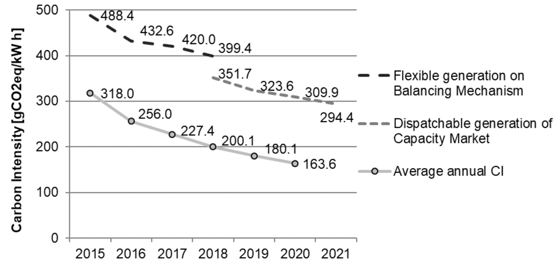
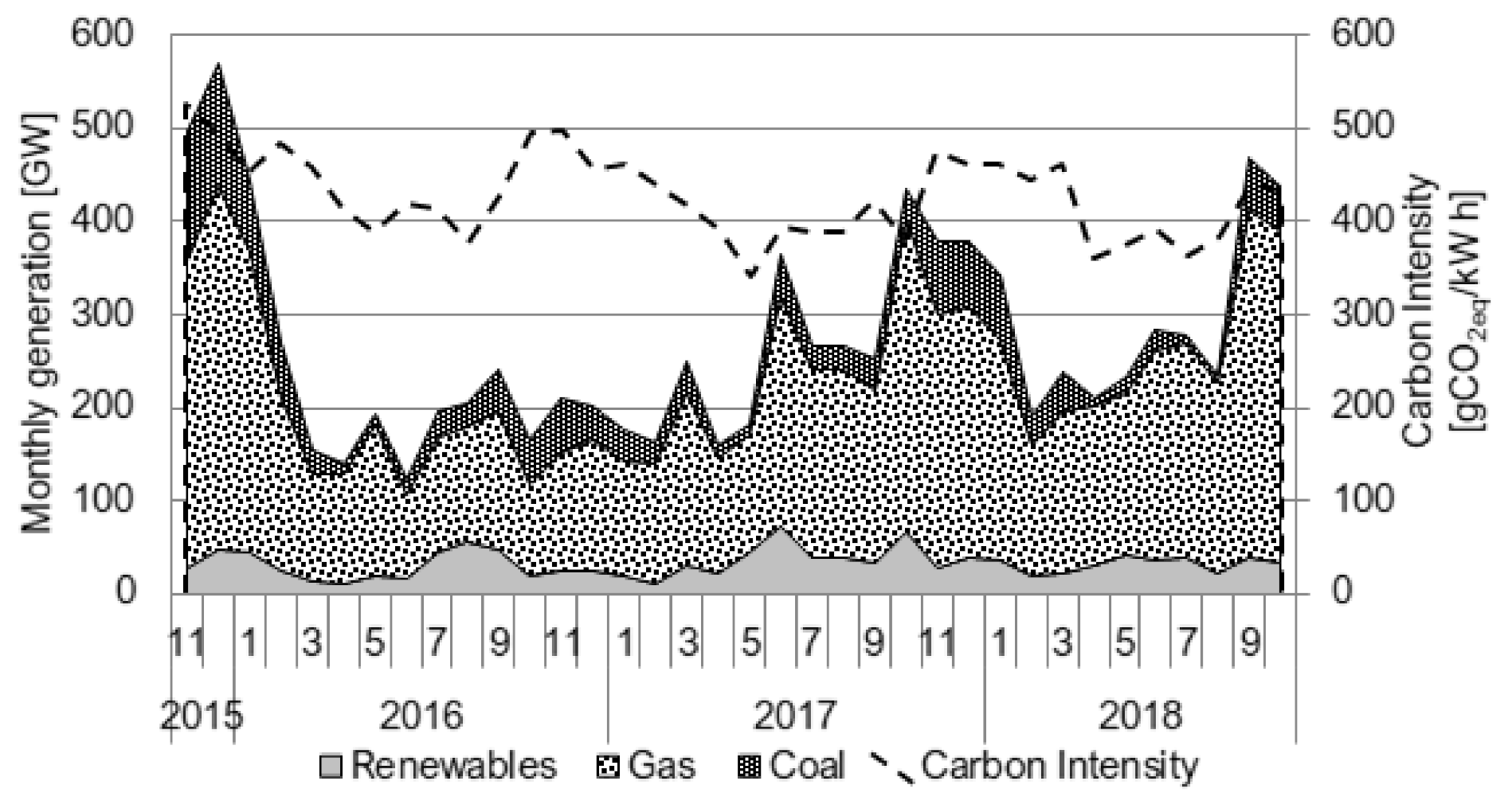
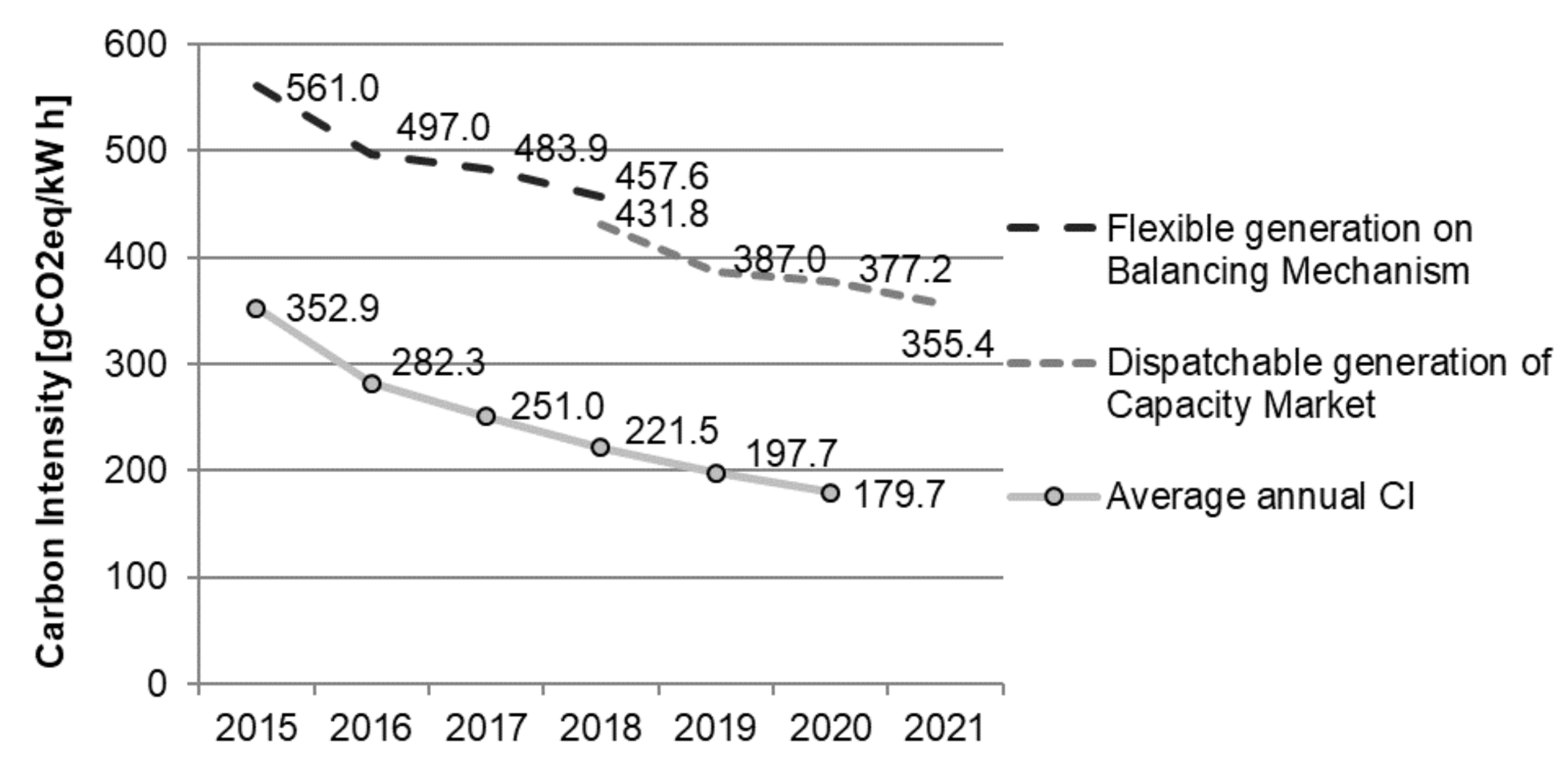
3.2. The Carbon Cost of Balancing Services

The CI per fuel values calculated according to the method detailed in Section 2 are presented in Table 3, in comparison with literature references. Values for fossil fuels are generally consistent with previous references. The small differences reflect the recent trends in use of the fuels. However, as discussed in Section 2, the values for the “other” renewables are notably different—this article presents the CI for each fuel based on scope-1 emissions, whilst previous authors use scope-1 for fossil-fuelled generation but scope-1 plus scope-3 for the “other” bioenergy sources.
The average CI of imports is 57 ± 1 gCO2eq/kW·h if from France, 464 ± 44 if from The Netherlands, 415 ± 58 if from Northern Ireland, 396 ± 50 if from the Republic of Ireland or 187 ± 19 when imported from Belgium [83]. The differences between the CI of these countries are due to the fuel mix used; for example, the fuel mix in France has a large contribution of LCTs (such as nuclear and hydro) while The Netherlands largely uses fossil fuels (including natural gas and coal).
The average CI of balancing services and the grid as a whole is shown clearly in Figure 3. Although all trends are decreasing, the gap between the average CI for the grid and both BM and CM values is increasing in the recent years. This is mainly because of the replacement of coal with natural gas, and that the uptake of LCTs has not progressed in the balancing services as fast as for the grid. Additionally, the CI of the grid is higher than the official figures because Elexon [55] only include generators connected to the transmission system and underestimate the contribution of renewables. In contrast, the CI of the BM and CM calculated in this work is underestimated. The values presented in Table 3 are based on the yearly average efficiency of each generation technology whereas in reality the efficiency of each generation plant varies with time according to the load. Generally, the efficiency of flexible capacity is reduced in comparison with steady generation [87,88]. Future assessments of the CI should take into consideration the variable efficiency of the power plants and overall emissions.
In the development of a net-zero carbon emissions electricity sector, emissions due to other stages of the lifecycle of a power plant become significant [10]. Therefore, as the share of LCT increase, the adoption of a consistent accounting method for scope-1 and scope-3 emissions for all fuels becomes more important. As additional contribution of this work, the estimation of CI accounting for scope-1 and scope-3 emission is detailed in Appendix A to clearly show the relevance of adding scope-3 emissions to future analysis, and the importance of using a consistent methodology for all fuels. Additionally, sustainable development demands that a wider range of impacts, other than carbon, are considered. In order to identify the technologies with the lowest overall impact, other methodologies need to be used, such as a full lifecycle assessment [89,90].
In GB, the balancing services use very little power from low-carbon sources. Both the BM and the CM are fossil-fuel dependent. In fact, fossil-fuelled power stations provide 69% of capacity of CM and 84% of generation on the BM.
Reliable LCTs capacity contributes for just 21% of the overall capacity agreed on CM: 6% is provided by renewable generators and 15% from nuclear power [56,59]. The remaining 10% is provided by interconnectors. Additionally, as most of the capacity is provided by existing generators (86%) and a marginal average of 5% of capacity is awarded to new generators of whatever type [57,60], the CM has, in the past, failed to support the uptake of low-carbon dispatchable capacity supply.
Figure 4 summarises the results of the recent T-4 auctions and shows the average CM’s CI. In addition to the auction held in 2014 for delivery year 2018/2019, another auction was held in 2017. The combined average CI of capacity delivered in 2018/2019 was 359.7 gCO2eq/kW·h, almost double the grid’s annual CI average in 2018. Additionally, the CI figure is underestimated as DSR and storage are discounted.
Similarly, LCTs make a limited contribution to the BM. Figure 5 shows the contribution of fuels to increasing (offers, internal circle) or decreasing (bids, external circle) generation, as an effect of trading within the BM during the PAR50 reference period. While LCTs make a small contribution of RES to positive generation, these have a greater role when a reduction in generation is required. In fact, 10.9% of accepted offers and 30.3% of bids are provided by renewable generators. To achieve decarbonisation, it would be desirable for this disparity to be eliminated or even reversed. When considering only the positive generation delivered to the BM, the CI did not decrease as much as the grid’s CI in the same period. Figure 6 shows trends of net positive generation provided by the BM per fuel and relative CI. The largest share of generation is from fossil-fuelled power stations, and RES generation is only marginal. This combination of fossil-fuelled and low-carbon generation affects the trends of CI.
In conclusion, low-carbon generators have a low level of participation in the balancing services. Consequently, efforts to achieve affordable SoES increase the overall emissions of the power system. This situation thus constitutes a drag on the overall decarbonisation trend for the electricity supply system.

3.3. Summary and Discussion of the Results

Current decarbonisation policies in GB are successfully driving a progressive replacement of fossil-fuelled generation towards low-carbon electricity sources. Because of the incentivisation schemes in place, LCTs for bulk electricity supply are becoming economically self-sustaining and produce electricity more cheaply than fossil-fuelled power stations [91]. However, the analysis of balancing services presented in this work provided figures for the economic and environmental trade-offs caused by the continued use of fossil fuels both in the CM and in the BM. These are summarised in Table 4, in comparison with reference values of the grid.
With the level of RES penetration in GB being 33%, the combined economic cost of SoES is estimated at GBP 5.60/MW·h. This adds a modest 5% to the overall cost of electricity and correlates to GBP 27.64 per year per domestic consumer. Hence, SoES is currently achieved without a significant impact on affordability. By contrast, the CI of balancing services is almost double the average grid’s CI, and flexible generation via the BM alone accounts for 5% of total emissions. Given this systemic reliance of SoES on fossil-fuelled generation, balancing services appear to be a “hard to decarbonise” subsector.
Decarbonisation of flexible active generation provided by balancing services is technically feasible, although the potential has not yet been exploited. In the GB geographical and natural environment context, the focus is on hydro and bioenergy power stations. Statistics show that nearly 2 GW and 8 GW of capacity exist as hydro and thermal power generation, respectively, from the combustion of biomass and wastes [72]. This means that low-carbon flexible capacity is double the maximum capacity needed on the BM, despite being used for a minimal 10.9% of generation.
As no significant technological barrier exists, market preference for flexible generation from fossil fuels appears to lie mainly within economic criteria. Research shows that the upscaling of low-carbon technologies is limited by the capital investment required [28,29] as RES in particular typically have high capital costs, but low operating costs. Bulk generation from RES spreads the high capital investment over a large output and therefore has lower costs than fossil-fuelled generation [91]. In contrast, for operation in the balancing services, generation and hence capacity factors are low. Fossil-fuelled generation increasingly finds its natural position as peaking power in the generation merit order, and similarly it has been outcompeting RES in the even “peakier” balancing markets.

4. Discussion: Policy Interventions and Wider Applicability

The results presented in this article highlight that an integrated policy on SoES that also encompasses decarbonisation, with continued attention to affordability, is needed to support the energy transition. This article used details of GB as a case study.
Possible policy suggestions for GB lie in improving the current BM and CM schemes. The CM contains only high-level restrictions for carbon emissions as requested by the EU’s directive on the internal market of electricity [92]; however, the carbon impact is not currently taken into account in selection of generators chosen to operate within the CM. Instead, the technology-neutrality of the CM could be amended to introduce a reserved pot for LCTs. For example, auctions that separately award capacity contracts for LCTs and carbon-intensive power stations might incentivise innovation and capital investment to reduce both carbon impact and dependency on carbon-intensive resources. Alternatively, a carbon intensity merit order criterion could be added to existing criteria both on the CM and BM, thus also encouraging the move towards decarbonisation.
The impacts on carbon emissions of an integrated policy are expected to be immediate and significant, while also supporting a progressive replacement of fossil-fuelled generation with low-carbon sources needed to complete the achievement of a fully decarbonised power system. The net-zero emissions strategy for Great Britain sets an ambitious but necessary goal. Although the CCC [45] considers net-zero emissions achievable by 2050 within the expected cost already accepted by the Government with the Climate Change Act (2008), additional incentivisation to support the uptake of flexible low-carbon generation technologies may come at a cost.
Further analysis of the possible increase in balancing costs and impacts on affordability in the short-term should be undertaken, given the significance of electricity prices, especially for the most vulnerable in society. However, the modest share of balancing services in the overall cost of electricity suggests that an improved balance between the three dimensions of the Trilemma could be achieved without substantially impacting the dimension of affordability. Additionally, despite the incentivisation schemes increasing the cost for a specific period of time to stimulate innovation, the uptake of RES supported by incentivisation schemes have reduced the wholesale cost in the long term [93,94]. Hence, if such incentivisation policy would be able to replicate the merit order effect seen in the wholesale markets, the BM market prices may reduce in the long term.
All major economies are seeking to transition to low climate-related emissions, and the decarbonisation of the power sector tends to be an early target. The approach developed in this work and its broad findings are applicable to many large electricity grids worldwide, especially for those for which natural resources or geographical conditions limit the potential contribution by flexible renewable electricity generators, however, with the exception of power system already fully renewable. The World Energy Trilemma statistics [95] show that globally only a few European countries are in an advanced and balanced position between decarbonisation and SoES. This list includes the UK. In contrast, the analysis presented in this work demonstrates that also the UK still has an opportunity for further advances.
The need for an integrated policy has already been identified, for example, in Germany. The German Renewable Energy Sources Act (2012) established a premium for flexible reliable low-carbon generators, but it has three significant limitations: (1) in not assessing or planning the need for reliable capacity towards decarbonising the balancing services, (2) in the simplicity of providing a premium, which does not by itself integrate with affordability, and (3) in the specification that these reliable generators are only biogas-fuelled power stations.
Decarbonisation, SoES and sustainable development policies are still evolving in UK and many countries, and the concept formulated in this work could assist these efforts.

5. Conclusions

This work provides a robust and consistent economic and carbon analysis of electricity generation statistics of balancing services used for SoES in the highly decarbonised GB power system. While some studies in the literature [61,62,63,64,65,66] attempted an indirect statistical analysis of grid data to estimate the carbon factor of the marginal power, the original contribution of this work is in elaborating the direct analysis of the marginal markets, focusing on affordability, decarbonisation and SoES. As a byproduct, this work provides a new consistent dataset of CI per fuel, suggesting an improvement to the current global standard methodologies [79,80,81].
The economic and carbon analysis demonstrates the systemic reliance of the GB electricity system on fossil-fuelled power stations for providing security of supply, which poses an obstruction towards the development of a fully decarbonised power system. The results show that SoES services have a relatively higher carbon impact than the grid, and the gap is increasing. However, their impacts could be reduced by supporting the development of flexible generators from renewable sources.
Notwithstanding the availability of several low-carbon options for balancing services, most remain unable to penetrate the markets that have been designed to provide security of supply at lowest cost. Since the market chooses the less expensive fossil-fuelled options, there is limited exploitation of the alternative low-carbon flexible generation. This appears to be a clear example of the Trilemma. Consequently, national policies to provide financial incentives to support the high capital investments required by LCTs to become flexible and contribute towards SoES may be justified to maintain an affordable and secure system, while lowering emissions.

Author Contributions

Conceptualization: M.L. (Mauro Lafratta), M.L. (Matthew Leach), R.B.T., M.W. and J.L.; data curation: M.L. (Mauro Lafratta); formal analysis, M.L. (Mauro Lafratta); funding acquisition, R.B.T., E.G., S.K.O. and J.L.; investigation, M.L. (Mauro Lafratta); methodology, M.L. (Mauro Lafratta), M.L. (Matthew Leach) and M.W.; project administration, M.L. (Mauro Lafratta); resources, M.L. (Mauro Lafratta); supervision, R.B.T., M.W., E.G., S.K.O., A.S. and J.L.; validation, M.L. (Mauro Lafratta) and M.L. (Matthew Leach); visualization, M.L. (Mauro Lafratta), M.L. (Matthew Leach) and R.B.T.; writing—original draft, M.L. (Mauro Lafratta); writing—review and editing, M.L. (Mauro Lafratta), M.L. (Matthew Leach), R.B.T., M.W., E.G., S.K.O., A.S. and J.L. All authors have read and agreed to the published version of the manuscript.

Funding

Mauro Lafratta is registered on the Practitioner Doctorate in Sustainability programme of the University of Surrey, funded by Thames Water Utilities Limited with the support of the UK Engineering and Physical Sciences Research Council (grant number EP/G037612/1). The APC was funded by the University of Surrey.

Data Availability Statement

Restrictions apply to the availability of these data. Data were obtained from ELEXON Limited and are available at https://www.bmreports.com/bmrs/, https://api.bmreports.com/BMRS/ and https://www.elexonportal.co.uk/ with the permission of ELEXON Limited. Data were obtained from National Grid ESO and are available at https://demandforecast.nationalgrid.com/efs_demand_forecast/faces/DataExplorer under National Grid ESO Open Data policy. Data were obtained from Department for Business Energy and Industrial Strategy (BEIS) and are available at https://www.gov.uk/government/collections/digest-of-uk-energy-statistics-dukes and https://www.gov.uk/government/collections/final-uk-greenhouse-gas-emissions-national-statistics under Open Government Licence v3.0. Data were obtained from Department for Business Energy and Industrial Strategy (BEIS) and Department for Environment Food and Rural Affairs (DEFRA) and are available at https://www.gov.uk/government/collections/government-conversion-factors-for-company-reporting under Open Government Licence v3.0. All accessed on 26 November 2020.

Acknowledgments

Authors gratefully thank the University of Surrey and Thames Water Utilities Ltd. for their support in delivering the project. The authors would like to thank Angus Berry, Matthew Gee and Andrea Gysin for their helpful comments. The authors would like to thank the anonymous reviewers for their comments that helped improve the quality of the article. Permission from ELEXON Limited as intellectual property holder to use BMRS, BSC Website and ELEXON Portal data is gratefully acknowledged. Access and utilisation of datasets from National Grid ESO is supported by National Grid ESO Open Data.

Conflicts of Interest

The authors declare no conflict of interest.

Appendix A

Different methodologies can be used for the calculation of carbon intensities per fuel. Emissions can be assessed as direct emissions from the use of the fuel (scope-1) and for emissions due to extraction, refining and transportation of the fuel sources (scope-3). The emissions for fossil fuels are normally calculated following the consumption-based accounting methodology and therefore only based on the scope-1 emissions. On the contrary, emissions from generation from bioenergy sources (including biomass) are normally measured including both scope-1 and scope-3 emissions [68]. Generally, these different methodologies account for the single phase that accounts for the largest emissions [96]. However, the use of different methodologies for the calculation of the CIs per fuel ultimately leads to ignoring significant amount of scope-3 emissions for fossil fuels and inconsistencies.
The article presents the calculation of CI for all fuels following the methodology normally used for fossil fuels to retain comparability with previous references. This method used in the article is based only on scope-1 emissions for all fuels.
Alternatively, the usual methodology for the calculation of thermal renewables could be used for all fuels. This includes the calculation of carbon factors (CF) as the sum of scope-1 and scope-3 emissions (Equation (A1)) and follows the methodology described in the article for the other steps.
C a r b o n   F a c t o r f u e l = C F S c o p e   1 , f u e l + C F S c o p e   3 , f u e l  
By including both scope-1 and scope-3 emissions for electricity generation, these CIs per fuel lead to a consistent and more comprehensive accounting of overall emissions. Additionally, as scope-1 emissions are meant to progressively reduce with the increasing share of LCTs, the inclusion of all lifecycle emissions, and scope-3 emissions as first step, is increasingly significant in the development of a net zero emissions power system. This concept ultimately applies to the greenhouse gas emissions and environmental impacts for renewables, including wind [97], solar [98,99,100] and nuclear [101]. Currently, BEIS and DEFRA do not include these technologies in their accounting methodology [81].
Table A1 presents the CIs per fuel calculated in this study considering scope-1 emissions only or also including scope-3 emissions. With scope-3 emissions added, the figure for thermal renewables (named “Other (using a mix of bioenergy)” in Table A1) until 2 November 2017 matches the ones available in the literature. However, after that date, ELEXON reports separately the statistics of electricity generation from biomass and from other thermal renewable sources, and consequently this work provides two different reference figures for each of these sources. There is a significant difference between the CF calculated in this work and the one estimated by Bruce et al. [69] and Rogers and Parsons [70] since 2 November 2017. However, it is not possible to establish the reason because neither source provides the details of the methodology used for their estimation. Hence, the method described in this work is an original contribution in comparison with literature references cited.
Table A1. CIs per fuel and technology, calculated according to the methodology in Section 2. Scope-1 emissions are calculated in the article; however, scope-1 and scope-3 emissions are calculated with the same methodology and using Equation (A1) for the calculation of carbon factors in Equation (6). All values are in g CO2eq/kW·h.
Technology and Fuel UsedThis Work, Based on Scope-1This Work, Based on Scope-1 and Scope-3Staffell [68]Bruce et al. [69] and Rogers and Parson [70]
Combined Cycle Gas Turbine (using natural gas)393 ± 6449 ± 7394 ± 6394
Oil (using Fuel Oil)1170 ± 1911390 ± 229935 ± 122935
Coal (assuming ‘coal for electricity generation’ as fuel)942 ± 301096 ± 35937 ± 15937
Open Cycle Gas Turbine (using natural gas)656 ± 11748.5 ± 12651 ± 10651
Other (using a mix of bioenergy)Until 2 November 2017 (including biomass)28 ± 1126 ± 3120 ± 120120
Since 2 November 2017 (excluding biomass reported separately)1 ± 056 ± 2300
Biomass (using wood pellets)Since 2 November 201753 ± 5180 ± 6120
Pumped hydro storage 1291 ± 97 1306 ± 110 1Not included0
1 Only for the assessment of the CI of the BM.
The carbon intensities calculated with the consistent methodology including scope-1 and scope-3 emissions are presented in Figure A1.
Figure A1. Carbon intensities of BM, CM and grid including scope-1 and scope-3.
Energies 14 05123 g0a1

References

  1. World Commission on Environment and Development. Our Common Future; Oxford University Press: Oxford, UK, 1987. [Google Scholar]
  2. United Nations General Assembly. The Future We Want—UN Resolution 66/288 Resolution Adopted by the General Assembly on 27 July 2012; United Nations: New York, NY, USA, 2012; p. 53. [Google Scholar]
  3. International Atomic Energy Agency; United Nations Department of Economic and Social Affairs; International Energy Agency; Eurostat; European Environment Agency. Energy Indicators for Sustainable Development: Guidelines and Methodologies; IAEA: Vienna, Austria, 2005. [Google Scholar]
  4. World Energy Council. World Energy Trilemma: Priority Actions on Climate Change and how to Balance the Trilemma; World Energy Council: London, UK, 2015. [Google Scholar]
  5. Fankhauser, S.; Tepic, S. Can poor consumers pay for energy and water? An affordability analysis for transition countries. Energy Policy 2007, 35, 1038–1049. [Google Scholar] [CrossRef]
  6. The European Parliament; The Council of the European Union. Directive 2005/89/EC of the European Parliament and of the Council of 18 January 2006 Concerning Measures to Safeguard Security of Electricity Supply and Infrastructure Investment (Text with EEA Relevance); Official Journal of the European Union; Publications Office of the European Union: Luxembourg, 2006; pp. 22–29. [Google Scholar]
  7. Helm, D. Energy policy: Security of supply, sustainability and competition. Energy Policy 2002, 30, 173–184. [Google Scholar] [CrossRef]
  8. Heptonstall, P.; Gross, R.; Steiner, F. The Costs and Impacts of Intermittency—2016 Update; UK Energy Research Centre: London, UK, 2017. [Google Scholar]
  9. Leslie, J. Zero Carbon Operation 2025; National Grid ESO: Warwick, UK, 2019; p. 4. [Google Scholar]
  10. Intergovernmental Panel on Climate Change. Climate Change 2014: Mitigation of Climate Change. Contribution of Working Group III to the Fifth Assessment Report of the Intergovernmental Panel on Climate Change; Cambridge University Press: Cambridge, UK; New York, NY, USA, 2014; 1435p. [Google Scholar]
  11. Lund, P.D.; Lindgren, J.; Mikkola, J.; Salpakari, J. Review of energy system flexibility measures to enable high levels of variable renewable electricity. Renew. Sustain. Energy Rev. 2015, 45, 785–807. [Google Scholar] [CrossRef] [Green Version]
  12. Huber, M.; Dimkova, D.; Hamacher, T. Integration of wind and solar power in Europe: Assessment of flexibility requirements. Energy 2014, 69, 236–246. [Google Scholar] [CrossRef] [Green Version]
  13. Papaefthymiou, G.; Dragoon, K. Towards 100% renewable energy systems: Uncapping power system flexibility. Energy Policy 2016, 92, 69–82. [Google Scholar] [CrossRef]
  14. Liebensteiner, M.; Wrienz, M. Do Intermittent Renewables Threaten the Electricity Supply Security? Energy Econ. 2019, 87, 104499. [Google Scholar] [CrossRef]
  15. Brouwer, A.S.; van den Broek, M.; Seebregts, A.; Faaij, A. Impacts of large-scale Intermittent Renewable Energy Sources on electricity systems, and how these can be modeled. Renew. Sustain. Energy Rev. 2014, 33, 443–466. [Google Scholar] [CrossRef]
  16. Ummels, B.C.; Gibescu, M.; Pelgrum, E.; Kling, W.L.; Brand, A.J. Impacts of Wind Power on Thermal Generation Unit Commitment and Dispatch. IEEE Trans. Energy Convers. 2007, 22, 44–51. [Google Scholar] [CrossRef] [Green Version]
  17. Gowrisankaran, G.; Reynolds, S.S.; Samano, M. Intermittency and the Value of Renewable Energy. J. Political Econ. 2016, 124, 1187–1234. [Google Scholar] [CrossRef] [Green Version]
  18. Grave, K.; Paulus, M.; Lindenberger, D. A method for estimating security of electricity supply from intermittent sources: Scenarios for Germany until 2030. Energy Policy 2012, 46, 193–202. [Google Scholar] [CrossRef]
  19. National Renewable Energy Laboratory. Western Wind and Solar Integration Study; National Renewable Energy Laboratory U.S. Department of Energy: Golden, CO, USA, 2010; p. 536.
  20. Lew, D.; Brinkman, G.; Ibanez, E.; Florita, A.; Heaney, M.; Hodge, B.M.; Gross, R.; Steiner, F. The Western Wind and Solar Integration Study Phase 2; National Renewable Energy Laboratory—U.S. Department of Energy: Golden, CO, USA, 2013; p. 244.
  21. Lund, H. Large-scale integration of wind power into different energy systems. Energy 2005, 30, 2402–2412. [Google Scholar] [CrossRef]
  22. Traber, T.; Kemfert, C. Gone with the wind?—Electricity market prices and incentives to invest in thermal power plants under increasing wind energy supply. Energy Econ. 2011, 33, 249–256. [Google Scholar] [CrossRef] [Green Version]
  23. Sahin, C.; Shahidehpour, M.; Erkmen, I. Generation risk assessment in volatile conditions with wind, hydro, and natural gas units. Appl. Energy 2012, 96, 4–11. [Google Scholar] [CrossRef]
  24. Bessa, R.; Moreira, C.; Silva, B.; Matos, M. Handling renewable energy variability and uncertainty in power systems operation. Wiley Interdiscip. Rev. Energy Environ. 2014, 3, 156–178. [Google Scholar] [CrossRef]
  25. Galvan, E.; Mandal, P.; Haque, A.U.; Tseng, T.-L. Optimal Placement of Intermittent Renewable Energy Resources and Energy Storage System in Smart Power Distribution Networks. Electr. Power Compon. Syst. 2017, 45, 1543–1553. [Google Scholar] [CrossRef]
  26. Weitemeyer, S.; Kleinhans, D.; Vogt, T.; Agert, C. Integration of Renewable Energy Sources in future power systems: The role of storage. Renew. Energy 2015, 75, 14–20. [Google Scholar] [CrossRef] [Green Version]
  27. Strbac, G. Demand side management: Benefits and challenges. Energy Policy 2008, 36, 4419–4426. [Google Scholar] [CrossRef]
  28. Lauer, M.; Dotzauer, M.; Hennig, C.; Lehmann, M.; Nebel, E.; Postel, J.; Kleinhans, D.; Vogt, T. Flexible power generation scenarios for biogas plants operated in Germany: Impacts on economic viability and GHG emissions. Int. J. Energy Res. 2016, 41, 63–80. [Google Scholar] [CrossRef] [Green Version]
  29. Szarka, N.; Scholwin, F.; Trommler, M.; Fabian Jacobi, H.; Eichhorn, M.; Ortwein, A.; Dotzauer, M.; Lehmann, M. A novel role for bioenergy: A flexible, demand-oriented power supply. Energy 2013, 61, 18–26. [Google Scholar] [CrossRef]
  30. Knorr, K.; Zimmermann, B.; Kirchner, D.; Speckmann, M.; Spieckermann, R.; Widdel, M.; Wunderlich, M.; Mackensen, R.; Rohrig, K.; Steinke, F.; et al. Kombikraftwerk 2—Final Report; Fraunhofer Institute for Energy Economics and Energy System Technology: Kassel, Germany, 2014; p. 218. [Google Scholar]
  31. Alizadeh, M.I.; Parsa Moghaddam, M.; Amjady, N.; Siano, P.; Sheikh-El-Eslami, M.K. Flexibility in future power systems with high renewable penetration: A review. Renew. Sustain. Energy Rev. 2016, 57, 1186–1193. [Google Scholar] [CrossRef]
  32. Hahn, H.; Krautkremer, B.; Hartmann, K.; Wachendorf, M. Review of concepts for a demand-driven biogas supply for flexible power generation. Renew. Sustain. Energy Rev. 2014, 29, 383–393. [Google Scholar] [CrossRef]
  33. Persson, T.; Murphy, J.D.; Jannasch, A.-K.; Ahern, E.; Liebetrau, J.; Trommler, M.; Parsa Moghaddam, M.; Amjady, N. A Perspective on the Potential Role of Biogas in Smart Energy Grids; Baxter, D., Ed.; IEA Bioenergy: Paris, France, 2014. [Google Scholar]
  34. Lafratta, M.; Thorpe, R.B.; Ouki, S.K.; Shana, A.; Germain, E.; Willcocks, M.; Lee, J. Dynamic biogas production from anaerobic digestion of sewage sludge for on-demand electricity generation. Bioresour. Technol. 2020, 310, 123415. [Google Scholar] [CrossRef] [PubMed]
  35. Lafratta, M.; Thorpe, R.B.; Ouki, S.K.; Shana, A.; Germain, E.; Willcocks, M.; Lee, J. Demand-Driven Biogas Production from Anaerobic Digestion of Sewage Sludge: Application in Demonstration Scale. Waste Biomass Valorization 2021. [Google Scholar] [CrossRef]
  36. Meeus, L.; Purchala, K.; Belmans, R. Development of the internal electricity market in Europe. Electr. J. 2005, 18, 25–35. [Google Scholar] [CrossRef]
  37. van der Veen, R.A.; Hakvoort, R.A. The electricity balancing market: Exploring the design challenge. Util. Policy 2016, 43, 186–194. [Google Scholar] [CrossRef] [Green Version]
  38. Black, M.; Strbac, G. Value of storage in providing balancing services for electricity generation systems with high wind penetration. J. Power Sources 2006, 162, 949–953. [Google Scholar] [CrossRef]
  39. Guinot, B.; Montignac, F.; Champel, B.; Vannucci, D. Profitability of an electrolysis based hydrogen production plant providing grid balancing services. Int. J. Hydrogen Energy 2015, 40, 8778–8787. [Google Scholar] [CrossRef]
  40. Joos, M.; Staffell, I. Short-term integration costs of variable renewable energy: Wind curtailment and balancing in Britain and Germany. Renew. Sustain. Energy Rev. 2018, 86, 45–65. [Google Scholar] [CrossRef]
  41. Gianfreda, A.; Parisio, L.; Pelagatti, M. A review of balancing costs in Italy before and after RES introduction. Renew. Sustain. Energy Rev. 2018, 91, 549–563. [Google Scholar] [CrossRef] [Green Version]
  42. Clauß, J.; Stinner, S.; Solli, C.; Lindberg, K.B.; Madsen, H.; Georges, L. Evaluation method for the hourly average CO2eq. Intensity of the electricity mix and its application to the demand response of residential heating. Energies 2019, 12, 1345. [Google Scholar] [CrossRef] [Green Version]
  43. Yin, R.K. Case Study Research: Design and Methods, 5th ed.; SAGE Publications, Inc.: Los Angeles, CA, USA, 2013. [Google Scholar]
  44. Castro, M. Assessing the risk profile to security of supply in the electricity market of Great Britain. Energy Policy 2017, 111, 148–156. [Google Scholar] [CrossRef]
  45. Committee on Climate Change. Net Zero: The UK’s Contribution to Stopping Global Warming; Committee on Climate Change: London, UK, 2019. [Google Scholar]
  46. Committee on Climate Change. The Sixth Carbon Budget: The UK’s Path to Net Zero; Committee on Climate Change: London, UK, 2020. [Google Scholar]
  47. Department for Business Energy & Industrial Strategy. Consolidated Version of the Capacity Market Rules; The National Archives: London, UK, 2017; p. 193. [Google Scholar]
  48. ELEXON Limited. The Balancing and Settlement Code. Consolidated Operational version; Version 15; ELEXON Limited: London, UK, 2001; p. 979. [Google Scholar]
  49. Office of Gas and Electricity Markets. Balancing and Settlement Code (BSC) P305: Electricity Balancing Significant Code Review Developments; OFGEM: London, UK, 2015; p. 16. [Google Scholar]
  50. Rodriguez-Alvarez, A.; Orea, L.; Jamasb, T. Fuel poverty and Well-Being: A consumer theory and stochastic frontier approach. Energy Policy 2019, 131, 22–32. [Google Scholar] [CrossRef] [Green Version]
  51. Liddell, C.; Morris, C.; McKenzie, S.J.P.; Rae, G. Measuring and monitoring fuel poverty in the UK: National and regional perspectives. Energy Policy 2012, 49, 27–32. [Google Scholar] [CrossRef]
  52. Vincent, L. Total Household Expenditure on Energy; Department for Business Energy & Industrial Strategy: London, UK, 2018.
  53. Office of Gas and Electricity Markets (OFGEM). State of the Energy Market 2019. State of the Energy Market; OFGEM: London, UK, 2019; p. 181. [Google Scholar]
  54. ELEXON Limited. Balancing Mechanism Reporting Service Dataset. Available online: https://api.bmreports.com/BMRS/ (accessed on 26 November 2020).
  55. ELEXON Limited. Balancing Mechanism Reporting Service. Available online: https://www.bmreports.com/bmrs/ (accessed on 26 November 2020).
  56. National Grid. Final Auction Results—T-4 Capacity Market Auction for 2019/20. 2015, p. 20. Available online: https://www.emrdeliverybody.com/Capacity%20Markets%20Document%20Library/T-4%20Final%20Results%202015.pdf (accessed on 26 November 2020).
  57. National Grid. Final Auction Results—T-1 Capacity Market Auction for 2018/19. 2018, p. 20. Available online: https://www.emrdeliverybody.com/Capacity%20Markets%20Document%20Library/Final%20Results%20T-1%202017%20(13.02.2018).pdf (accessed on 26 November 2020).
  58. National Grid. Final Auction Results—T-4 Capacity Market Auction 2014. 2014, p. 42. Available online: https://www.emrdeliverybody.com/Capacity%20Markets%20Document%20Library/T-4%202014%20Final%20Auction%20Results%20Report.pdf (accessed on 26 November 2020).
  59. National Grid. Final Auction Results—T-4 Capacity Market Auction for 2020/21. 2016, p. 26. Available online: https://www.emrdeliverybody.com/Capacity%20Markets%20Document%20Library/Final%20Results%20Report%20-%20T-4%202016.pdf (accessed on 26 November 2020).
  60. National Grid. Final Auction Results—T-4 Capacity Market Auction for 2021/22. 2018, p. 31. Available online: https://www.emrdeliverybody.com/Capacity%20Markets%20Document%20Library/Final%20T-4%20Results%20(Delivery%20Year%2021-22)%2020.02.2018.pdf (accessed on 26 November 2020).
  61. Hawkes, A.D. Estimating marginal CO2 emissions rates for national electricity systems. Energy Policy 2010, 38, 5977–5987. [Google Scholar] [CrossRef]
  62. Siler-Evans, K.; Lima Azevedo, I.; Morgan, M.G. Marginal Emissions Factors for the U.S. Electricity System. Environ. Sci. Technol. 2012, 46, 4742–4748. [Google Scholar] [CrossRef] [PubMed]
  63. Hawkes, A.D. Long-run marginal CO2 emissions factors in national electricity systems. Appl. Energy 2014, 125, 197–205. [Google Scholar] [CrossRef] [Green Version]
  64. Zheng, Z.; Han, F.; Li, F.; Zhu, J. Assessment of marginal emissions factor in power systems under ramp-rate constraints. CSEE J. Power Energy Syst. 2015, 1, 37–49. [Google Scholar] [CrossRef]
  65. Böing, F.; Regett, A. Hourly CO2 Emission Factors and Marginal Costs of Energy Carriers in Future Multi-Energy Systems. Energies 2019, 12, 2260. [Google Scholar] [CrossRef] [Green Version]
  66. Huber, J.; Lohmann, K.; Schmidt, M.; Weinhardt, C. Carbon efficient smart charging using forecasts of marginal emission factors. J. Clean. Prod. 2021, 284, 124766. [Google Scholar] [CrossRef]
  67. National Grid ESO. Connection and Use of System Code; National Grid ESO: Warwick, UK, 2020; p. 135. [Google Scholar]
  68. Staffell, I. Measuring the progress and impacts of decarbonising British electricity. Energy Policy 2017, 102, 463–475. [Google Scholar] [CrossRef] [Green Version]
  69. Bruce, A.R.W.; Ruff, L.; Kelloway, J.; MacMillan, F.; Rogers, A. Carbon Intensity Forecast Methodology. National Grid ESO: Warwick, UK. Available online: https://github.com/carbon-intensity/methodology/raw/master/Carbon%20Intensity%20Forecast%20Methodology.pdf (accessed on 26 July 2021).
  70. Rogers, A.; Parson, O. GridCarbon: A Smartphone App to Calculate the Carbon Intensity of the UK Electricity Grid. Available online: https://www.cs.ox.ac.uk/people/alex.rogers/gridcarbon/gridcarbon.pdf (accessed on 26 November 2020).
  71. Department for Business Energy & Industrial Strategy (BEIS). Final UK Greenhouse Gas Emissions National Statistics 2020. In Final UK Greenhouse Gas Emissions National Statistics from 1990; The National Archives: London, UK, 2020. [Google Scholar]
  72. Department for Business Energy & Industrial Strategy (BEIS). Digest of UK Energy Statistics 2020; BEIS: London, UK, 2020. [Google Scholar]
  73. Department for Business Energy & Industrial Strategy (BEIS); Department for Environment Food & Rural Affairs (DEFRA). UK Government GHG Conversion Factors for Company Reporting. Government Conversion Factors for Company Reporting of Greenhouse Gas Emissions. 1 January 2015; The National Archives: London, UK, 2015.
  74. Department for Business Energy & Industrial Strategy (BEIS); Department for Environment Food & Rural Affairs (DEFRA). UK Government GHG Conversion Factors for Company Reporting. Government Conversion Factors for Company Reporting of Greenhouse Gas Emissions. 1 June 2016; The National Archives: London, UK, 2016.
  75. Department for Business Energy & Industrial Strategy (BEIS); Department for Environment Food & Rural Affairs (DEFRA). UK Government GHG Conversion Factors for Company Reporting. Government Conversion Factors for Company Reporting of Greenhouse Gas Emissions. 4 August 2017; The National Archives: London, UK, 2017.
  76. Department for Business Energy & Industrial Strategy (BEIS); Department for Environment Food & Rural Affairs (DEFRA). UK Government GHG Conversion Factors for Company Reporting. Government Conversion Factors for Company Reporting of Greenhouse Gas Emissions. 8 June 2018; The National Archives: London, UK, 2018.
  77. Department for Business Energy & Industrial Strategy (BEIS); Department for Environment Food & Rural Affairs (DEFRA). UK Government GHG Conversion Factors for Company Reporting. Government Conversion Factors for Company Reporting of Greenhouse Gas Emissions. 9 June 2020; The National Archives: London, UK, 2020.
  78. Department for Business Energy & Industrial Strategy (BEIS); Department for Environment Food & Rural Affairs (DEFRA). UK Government GHG Conversion Factors for Company Reporting. Government Conversion Factors for Company Reporting of Greenhouse Gas Emissions. 4 June 2019; The National Archives: London, UK, 2019.
  79. Intergovernmental Panel on Climate Change (IPCC). 2006 IPCC Guidelines for National Greenhouse Gas Inventories; Eggleston, H.S., Buendia, L., Miwa, K., Ngara, T., Tanabe, K., Eds.; National Greenhouse Gas Inventories Programme: Hayama, Japan, 2006. [Google Scholar]
  80. International Financial Institution Technical Working Group on Greenhouse Gas Accounting. GHG Accounting for Grid Connected Renewable Energy Projects; United Nations Framework Convention on Climate Change: Bonn, Germany, 2019. [Google Scholar]
  81. Department for Business Energy & Industrial Strategy (BEIS). 2019 Government Greenhouse Gas Conversion Factors for Company Reporting—Methodology Paper for Emission Factors Final Report; Hill, N., Karagianni, E., Jones, L., MacCarthy, J., Bonifazi, E., Hinton, S., Afais, P., Smith, J., Eds.; The National Archives: London, UK, 2019. [Google Scholar]
  82. Drax Group PLC. Annual Report and Accounts 2018: Enabling a Zero Carbon, Lower Cost Energy Future; Drax Group PLC: Selby, UK, 2019; p. 192. [Google Scholar]
  83. International Energy Agency. CO2 Emissions from Fuel Combustion 2017; International Energy Agency: Paris, France, 2017. [Google Scholar]
  84. European Environment Agency (EEA). CO2 Emission Intensity. Available online: https://www.eea.europa.eu/data-and-maps/daviz/co2-emission-intensity (accessed on 26 November 2020).
  85. Department of Agriculture Environment and Rural Affairs. Northern Ireland Carbon Intensity Indicators 2020; Department of Agriculture, Environment and Rural Affairs: Belfast, UK, 2020; p. 32.
  86. ELEXON Limited. ELEXON Portal. 2020. Available online: https://www.elexonportal.co.uk/ (accessed on 26 November 2020).
  87. Graf, C.; Marcantonini, C. Renewable energy and its impact on thermal generation. Energy Econ. 2017, 66, 421–430. [Google Scholar] [CrossRef]
  88. The Competition and Markets Authority. Energy Market Investigation—Wholesale Electricity Market Rules; The National Archives: London, UK, 2015; p. 30.
  89. BS EN ISO 14040. Environmental Management. Life Cycle Assessment. Principles and Framework; British Standards Institute: London, UK, 2006. [Google Scholar]
  90. BS EN ISO 14044, 2006+A1. Environmental Management. Life Cycle Assessment. Requirements and Guidelines; British Standards Institute: London, UK, 2018. [Google Scholar]
  91. International Renewable Energy Agency. Renewable Power Generation Costs in 2018; International Renewable Energy Agency: Abu Dhabi, United Arab Emirates, 2019. [Google Scholar]
  92. The European Parliament; The Council of the European Union. Regulation (EU) 2019/943 of the European Parliament and of the Council of 5 June 2019 on the Internal Market for Electricity (Text with EEA Relevance); Official Journal of the European Union; Publications Office of the European Union: Luxembourg, 2019; p. 70. [Google Scholar]
  93. Sensfuß, F.; Ragwitz, M.; Genoese, M. The merit-order effect: A detailed analysis of the price effect of renewable electricity generation on spot market prices in Germany. Energy Policy 2008, 36, 3086–3094. [Google Scholar] [CrossRef] [Green Version]
  94. Clò, S.; Cataldi, A.; Zoppoli, P. The merit-order effect in the Italian power market: The impact of solar and wind generation on national wholesale electricity prices. Energy Policy 2015, 77, 79–88. [Google Scholar] [CrossRef]
  95. World Energy Council. World Energy Trilemma Index Report 2020. Available online: Trilemma.worldenergy.org (accessed on 14 May 2021).
  96. Turconi, R.; Boldrin, A.; Astrup, T. Life cycle assessment (LCA) of electricity generation technologies: Overview, comparability and limitations. Renew. Sustain. Energy Rev. 2013, 28, 555–565. [Google Scholar] [CrossRef] [Green Version]
  97. Xie, J.-B.; Fu, J.-X.; Liu, S.-Y.; Hwang, W.-S. Assessments of carbon footprint and energy analysis of three wind farms. J. Clean. Prod. 2020, 254, 120159. [Google Scholar] [CrossRef]
  98. Zafrilla, J.-E.; Arce, G.; Cadarso, M.-Á.; Córcoles, C.; Gómez, N.; López, L.-A.; Marcantonini, C.; Zoppoli, P. Triple bottom line analysis of the Spanish solar photovoltaic sector: A footprint assessment. Renew. Sustain. Energy Rev. 2019, 114, 109311. [Google Scholar] [CrossRef]
  99. Desideri, U.; Proietti, S.; Zepparelli, F.; Sdringola, P.; Bini, S. Life Cycle Assessment of a ground-mounted 1778kWp photovoltaic plant and comparison with traditional energy production systems. Appl. Energy 2012, 97, 930–943. [Google Scholar] [CrossRef]
  100. Fthenakis, V.M.; Kim, H.C. Greenhouse-gas emissions from solar electric- and nuclear power: A life-cycle study. Energy Policy 2007, 35, 2549–2557. [Google Scholar] [CrossRef]
  101. Sovacool, B.K. Valuing the greenhouse gas emissions from nuclear power: A critical survey. Energy Policy 2008, 36, 2950–2963. [Google Scholar] [CrossRef]
Figure 1. BM daily prices’ average ranging from 1 April 2015 to 31 October 2020. Data source: [55]. PAR500 period ended in November 2015, PAR50 period ended in November 2018. In isolated instances, the price was higher than GBP 1000.00/MW·h, reaching GBP 1528.72/MW·h in February 2017, GBP 1509.80/MW·h in August 2017 and GBP 2242.31/MW·h in June 2020
Energies 14 05123 g001
Figure 2. Daily volumes traded on the BM (i.e., accepted bids and offers) in PAR50 period [54] and net market imbalance volume [86].
Energies 14 05123 g002
Figure 3. Carbon intensity of flexible generation on the BM and dispatchable generation secured in CM auctions, plotted against the average annual CI of the grid. The average annual value for 2020 is provisional.
Energies 14 05123 g003
Figure 4. Dispatchable capacity secured in T-4 CM auctions per technology and fuel [56,58,59,60] and estimated CI.
Energies 14 05123 g004
Figure 5. Increase (internal circle) and decrease (external circle) in generation by fuel on the BM during the PAR50 period. Data sourced from Elexon [54].
Energies 14 05123 g005
Figure 6. Active generation provided by the BM in PAR50 period per fuel and CI. Data source: [54].
Energies 14 05123 g006
Table 1. Clearing price, capacity awarded and total forecasted cost for CM auction [56,57,58,59,60].
Auction2014 T-42015 T-42016 T-42017 T-42017 T-1
Delivery year2018/192019/202020/212021/222018/19
Clear price [GBP/kW/year]19.4018.0022.508.406.00
Capacity [GW]49.346.352.450.45.8
Total cost [GBP]956 m834 m1179 m423 m35 m
Table 2. Average and standard deviation in different quarters of real market prices and recalculated market prices (i.e., when real market price is calculated with PAR500, the marginal prices is calculated with PAR50, and when the real market price is calculated with PAR50, the marginal price is calculated with PAR1). The standard deviation is assumed as an indicator of volatility. Prices are expressed in constant value terms. Data source: [86].
Period
(from–to, dd/mm/yy)
Real
PAR
Real Market PriceMarginal
PAR
Recalculated Market Price
Average
[GBP/MW·h]
Standard
Deviation
Average
[GBP/MW·h]
Standard
Deviation
01/02/201530/04/2015PAR500GBP 41.8838.31%PAR50GBP 43.2751.34%
01/05/201531/07/2015PAR500GBP 41.9038.79%PAR50GBP 42.9151.87%
01/08/201504/11/2015PAR500GBP 43.6747.41%PAR50GBP 46.1964.82%
05/11/201501/02/2016PAR50GBP 38.5453.68%PAR1GBP 38.9057.50%
02/02/201630/04/2016PAR50GBP 35.7984.26%PAR1GBP 36.3589.69%
01/05/201631/07/2016PAR50GBP 34.7872.66%PAR1GBP 34.9279.16%
01/08/201631/10/2016PAR50GBP 38.86107.95%PAR1GBP 39.99141.77%
01/11/201631/01/2017PAR50GBP 55.86129.88%PAR1GBP 57.17142.85%
01/02/201730/04/2017PAR50GBP 41.2959.85%PAR1GBP 41.5664.20%
01/05/201731/07/2017PAR50GBP 41.54108.36%PAR1GBP 42.00120.94%
01/08/201731/10/2017PAR50GBP 43.8053.45%PAR1GBP 44.1656.69%
01/11/201731/01/2018PAR50GBP 51.9641.27%PAR1GBP 52.1942.61%
01/02/201830/04/2018PAR50GBP 57.6280.36%PAR1GBP 57.6280.37%
01/05/201831/07/2018PAR50GBP 52.9838.14%PAR1GBP 52.9838.14%
01/08/201804/11/2018PAR50GBP 61.2839.60%PAR1GBP 61.2839.61%
Table 3. CIs for electricity generation per fuel and technology, calculated according to the methodology in Section 2. The category “other” includes bioenergy sources, with biomass calculated separately since 2 November 2017. All values are in g CO2eq/kW·h.
Technology and Fuel UsedThis Work, Based on Scope-1Staffell [68]Bruce et al. [69] and Rogers and Parson [70]
Combined Cycle Gas Turbine (using Natural Gas)393 ± 6394 ± 6394
Oil (using Fuel Oil)1170 ± 191935 ± 122935
Coal (assuming “coal for electricity generation” as fuel)942 ± 30937 ± 15937
Open Cycle Gas Turbine (using Natural Gas)656 ± 11651 ± 10651
Other (using a mix of bioenergy)Until 2 November 2017, including biomass28 ± 1120 ± 120120
Since 2 November 2017, excluding biomass reported separately1 ± 0300
Biomass (using wood pellets)Since 2 November 201753 ± 5120
Pumped hydro storage 1291 ± 97Not included0
1 The CI of PHS is used only for the assessment of the average CI of the BM.
Table 4. Summary of main indicators of economic and carbon costs of balancing services in comparison with the grid. The variation of CI of the CM refers to the year the auction took place.
GenerationOverall Estimated Daily CostCI in 2018
[g CO2eq/kW·h]
Variation of CI 2015–2018
BM8 TW·hGBP1.3 m399.4−18%
CM33 TW·hGBP2.7 m359.7−17%
Grid301 TW·hGBP100.5 m199.6−36%
Publisher’s Note: MDPI stays neutral with regard to jurisdictional claims in published maps and institutional affiliations.

