
Sustainable Water Supply Systems Management for Energy Efficiency: A Case Study

 , and
, and
Abstract
:1. Introduction
- − Pressure control: change in pump status (open/closed) along with a change in pressure in the network;
- − Level control: change in pump status according to water level variations in storage tanks;
- − Time controls: change in pump status at fixed hours of the day.
- −
- Top-down methodologies: focus on efficiency assessments concerning general and diverse processes of the water utility as well as macroeconomic analyses. A frequently used method is a benchmarking or energy audit. Examples of these methods and tools include: ECAM—Energy Performance and Carbon Emissions Assessment and Monitoring Tool; IBNET—the International Benchmarking Network; AquaRating (performance assessment system for water); EPA’s Energy Use Assessment Tool; Tools for Energy Footprint Assessment in Urban Water Systems.
- −
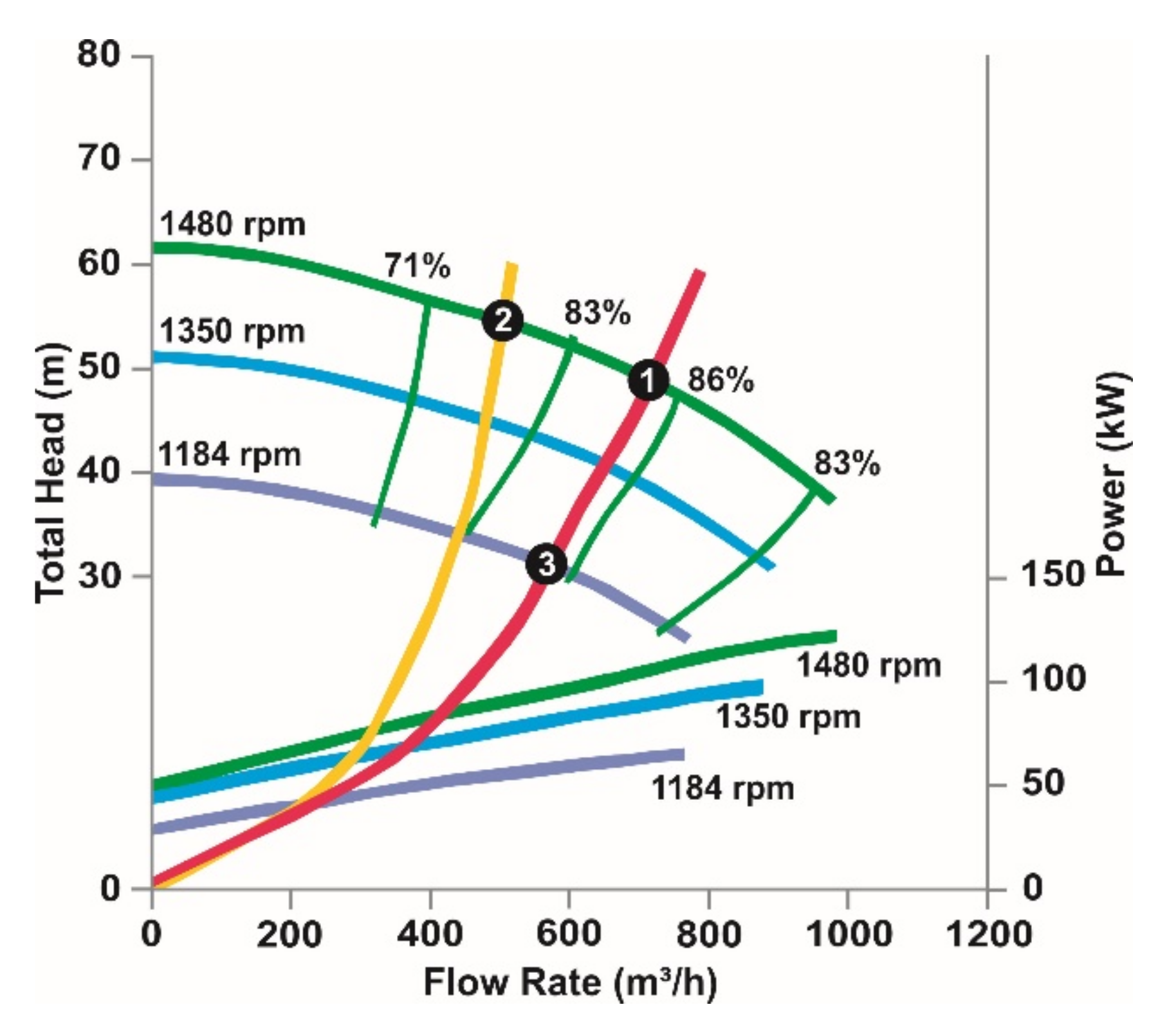
- Bottom-up methodologies: are more detailed, based in large part on an energy audit, an energy assessment that focuses on comparing the energy consumed in an ideal system and a real system. Mathematical modeling of operations and physical phenomena and processes are used to develop the ideal network, and the computer model EPANET [35] is often used. Hydraulic analyses are most often calculated using the Darcy–Weisbach equation or the Hazen–Williams equation or based on pump curves (pump efficiency estimation). Many methods based on bottom-up approaches focus on identifying and analyzing the causes of energy losses in water supply systems. Many metrics and indicators can be used to assess energy efficiency.
2. Materials and Methods
2.1. Research Object
2.1.1. Water Treatment Plant
2.1.2. Pumping Stations
- −
- PS N: If node number 13,545 pressure is below 43 mH2O, then pump number 20,965 status is open; if node number 13,545 pressure is below 40 mH2O, then pump number 20,966 status is open (cascade pumps switching)—pressure control,
- −
- PS L: If tank number 12,989 level is below 4.5 mH2O, then pump number 19,152 status is open, else pump number 19,152 status is closed—level control,
- −
- WTP F: If system clock time ≥6 a.m., and system clock time ≤10 p.m., then pump 21,141 status is open, else pump 21,141 status is closed—time control.
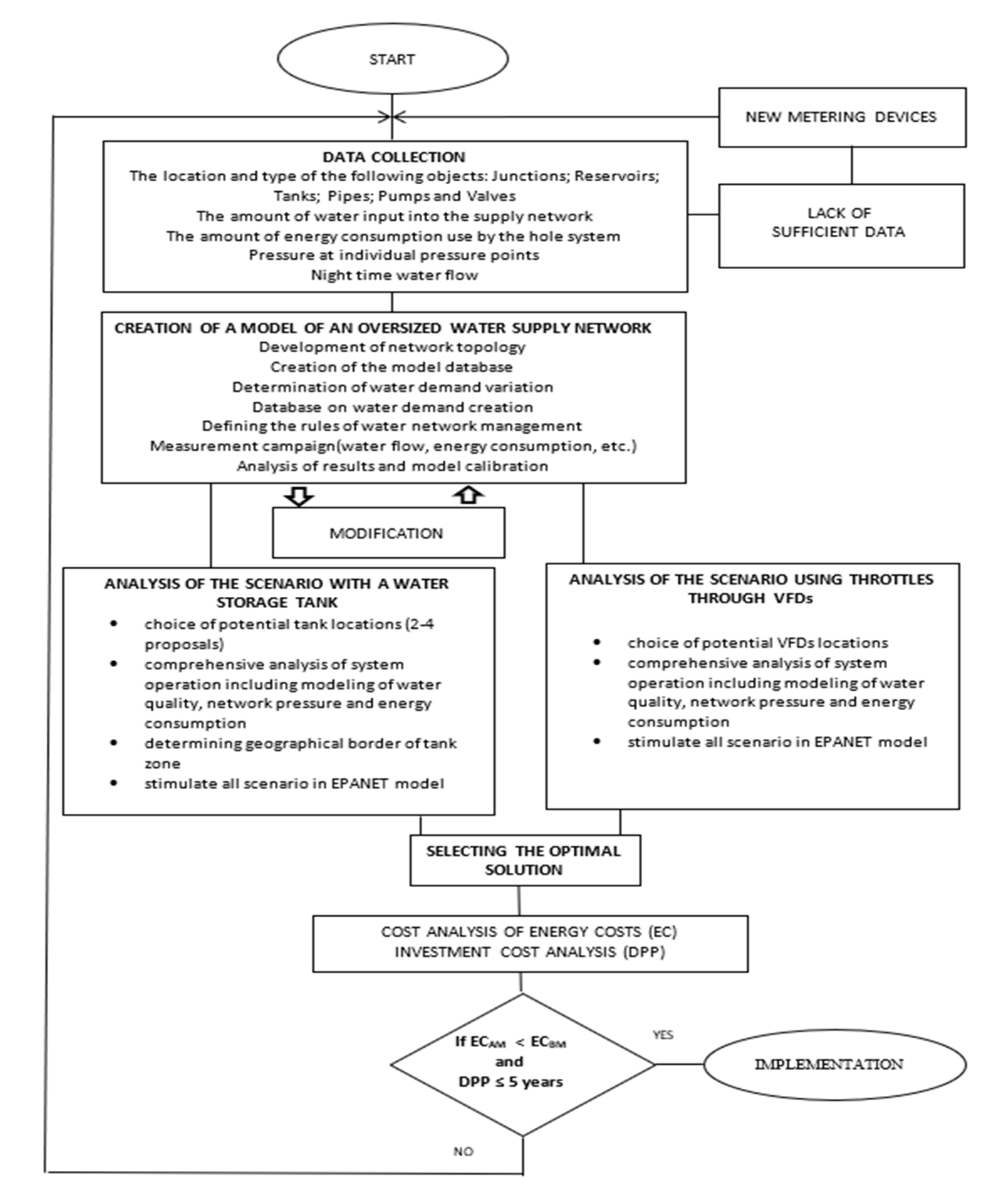
2.2. Analysis Methodology
3. Results and Discussion
- −
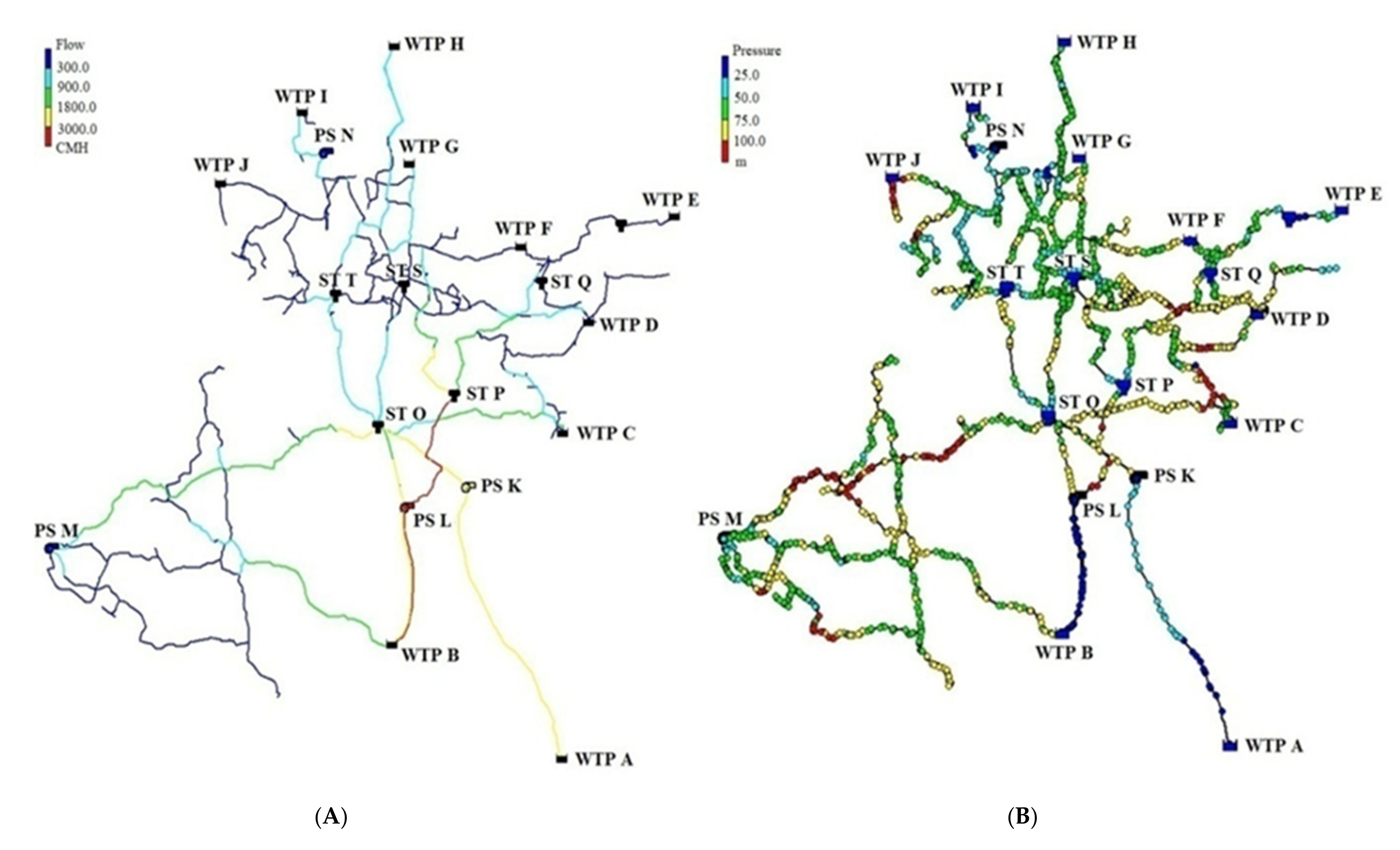
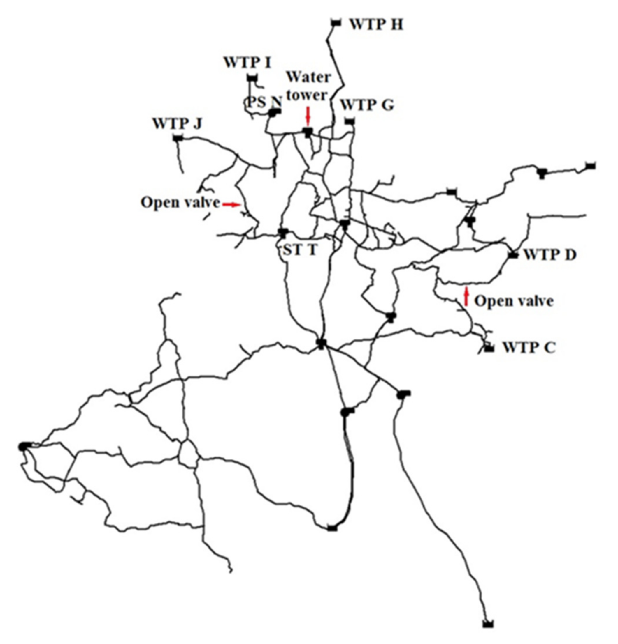
- The location and type of the following objects: junctions; reservoirs; tanks; pipes; pumps and valves;
- −
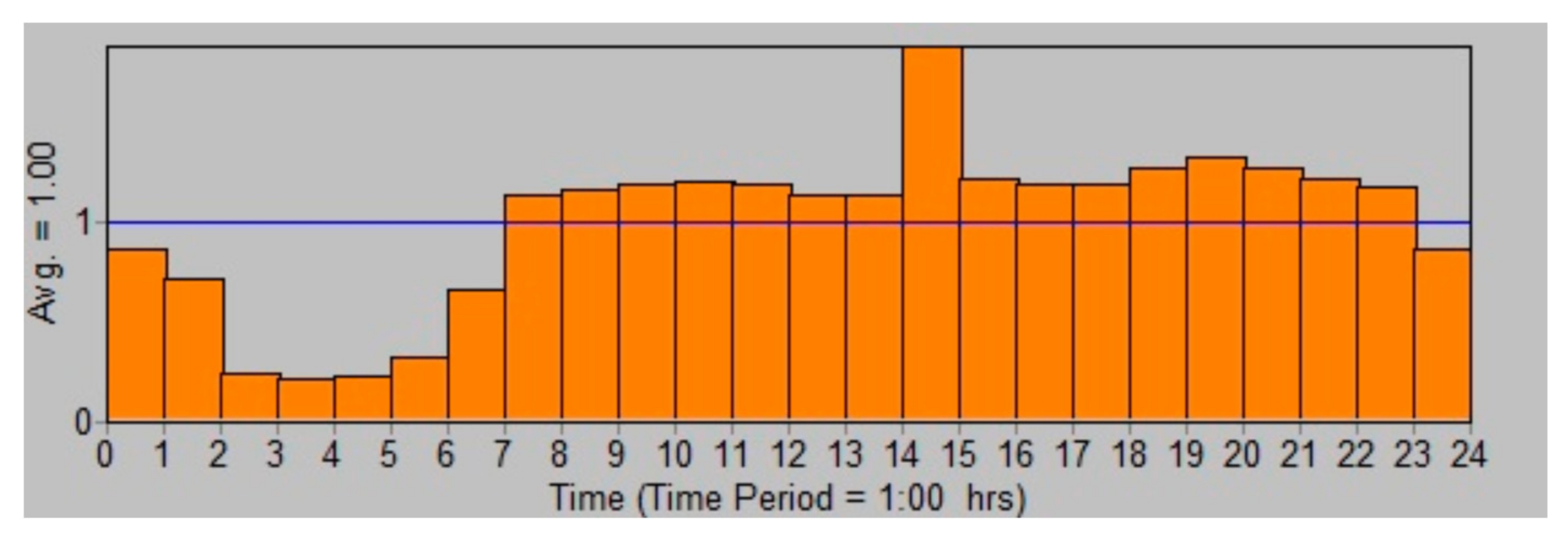
- The amount of water input into the supply network;
- −
- The amount of energy consumption used by the whole system;
- −
- Pressure at individual pressure points and nighttime water flow.
4. Conclusions
- An inventory of the current state of the pumping system in terms of hydraulic requirements and energy consumption.
- Analysis of the level of water losses accompanied by the identification of their source, analysis of water supply network failure rate, analysis, and classification of leakage levels (creation and ongoing maintenance of a database of failures and losses).
- Use of numerical simulation model EPANET 2.0 for the selection of optimal operating parameters under changing conditions of the water supply system (maximal and minimal hourly water demands, maximal and minimal pressure).
- Determination of critical operation zones of the water supply system, taking into account the optimization of pumping systems.
- Online monitoring of hydraulic parameters, including critical zones, and energy monitoring of pumping stations (creation and maintenance of a database of hydraulic and energy parameters).
- Development of indicator limits for the operational decision-making system.
- Ranking of investment needs in order to achieve the assumed energy effect.
Author Contributions
Funding
Informed Consent Statement
Conflicts of Interest
References
- Bluszcz, A.; Manowska, A. Differentiation of the Level of Sustainable Development of Energy Markets in the European Union Countries. Energies 2020, 13, 4882. [Google Scholar] [CrossRef]
- Hąbek, P. CSR Reporting Practices in Visegrad Group Countries and the Quality of Disclosure. Sustainability 2017, 9, 2322. [Google Scholar] [CrossRef] [Green Version]
- Dobrowolska, M.; Knop, L. Fit to Work in the Business Models of the Industry 4.0 Age. Sustainability 2020, 12, 4854. [Google Scholar] [CrossRef]
- Lam, K.L.; Kenway, S.J.; Lant, P.A. Energy use for water provision in cities. J. Clean. Prod. 2017, 143, 699–709. [Google Scholar] [CrossRef] [Green Version]
- Ramos, H.M.; Vieira, F.; Covas, D.I.C. Energy efficiency in a water supply system: Energy consumption and CO2 emission. Water Sci. Eng. 2010, 3, 331–340. [Google Scholar] [CrossRef]
- Hiremath, R.B.; Shikha, S.; Ravindranath, N.H. Decentralized energy planning; modeling and application—A review. Renew. Sustain. Energy Rev. 2007, 11, 729–752. [Google Scholar] [CrossRef]
- Carriço, N.; Covas, D.; Alegre, H.; do Céu Almeida, M. How to assess the effectiveness of energy management processes in water supply systems. J. Water Supply Res. Technol. 2014, 63. [Google Scholar] [CrossRef]
- Klosok-Bazan, I.; Machnik-Slomka, J. Crisis management in small water supply companies—Problem with water quality. In Proceedings of the International Multidisciplinary Scientific GeoConference: SGEM, Albena, Bulgaria, 2–8 July 2018; pp. 179–185. [Google Scholar]
- Zimoch, I.; Bartkiewicz, E. Optimization of energy cost in water supply system. E3S Web Conf. 2017, 22. [Google Scholar] [CrossRef] [Green Version]
- Porsinger, T.; Janik, P.; Leonowicz, Z.; Gono, R. Modelling and Optimization in Microgrids. Energies 2017, 10, 523. [Google Scholar] [CrossRef] [Green Version]
- Machnik-Słomka, J. Smart specialization as a factor stimulating innovative development of water and wastewater economy. E3S Web Conf. 2018, 59. [Google Scholar] [CrossRef] [Green Version]
- European Council, Conclusions—23/24 October 2014; EUCO 169/14; European Council: Brussels, Belgium, 2014.
- Directive 2009/28/EC of the European Parliament and of the Council of 23 April 2009 on the Promotion of the Use of Energy from Renewable Sources and Amending and Subsequently Repealing Directives 2001/77/EC and 2003/30/EC, L. 140/16; Official Journal of the European Union: Brussels, Belgium, 2009.
- Directive 2012/27/EU of the European Parliament and of the Council of 25 October 2012 on Energy Efficiency, Amending Directives 2009/125/EC and 2010/30/EU and Repealing Directives 2004/8/EC and 2006/32/EC, L.315/1; Official Journal of the European Union: Brussels, Belgium, 2012.
- European Commission: Accompanying the document Communication from the Commission to the European Parliament, the Council, the European Economic and Social Committee and the Committee of the Regions: A Policy Framework for Climate and Energy in the Period from 2020 to 2030; Official Journal of the European Union: Brussels, Belgium, 2014.
- Directive (EU) 2018/2002 of the European Parliament and of the Council of 11 December 2018 amending Directive 2012/27/EU on Energy Efficiency, L.328/210; Official Journal of the European Union: Brussels, Belgium, 2018.
- Klosok-Bazan, I.; Boguniewicz-Zablocka, J.; Suda, A.; Łukasiewicz, E.; Anders, D. Assessment of leakage management in small water supplies using performance indicators. Environ. Sci. Pollut. Res. 2021, 28, 41181–41190. [Google Scholar] [CrossRef] [PubMed]
- Matyjaszek, M.; Fidalgo Valverde, G.; Krzemień, A.; Wodarski, K.; Riesgo Fernández, P. Optimizing Predictor Variables in Artificial Neural Networks When Forecasting Raw Material Prices for Energy Production. Energies 2020, 13, 2017. [Google Scholar] [CrossRef] [Green Version]
- Zimoch, I.; Bartkiewicz, E. Analysis of disinfectant decay in a water supply system based on mathematical model. Desalin. Water Treat. 2018, 134. [Google Scholar] [CrossRef]
- Zimoch, I.; Bartkiewicz, E. Use of disinfection by-products (DBPs) generation simulation models in the risk analysis of secondary water contamination. Desalin. Water Treat. 2020, 199. [Google Scholar] [CrossRef]
- Alegre, H.; Coelho, S.T. Infrastructure Asset Management of Urban Water Systems. In Water Supply System Analysis—Selected Topics; InTech: London, UK, 2012. [Google Scholar]
- World Energy Outlook; International Energy Agency: Paris, France, 2016.
- Enrique, C.; Pardo, M.A.; Ricardo, C.; Enrique, C. Energy Audit of Water Networks. J. Water Resour. Plan. Manag. 2010, 136, 669–677. [Google Scholar] [CrossRef]
- Vilanova, M.R.N.; Balestieri, J.A.P. Modeling of hydraulic and energy efficiency indicators for water supply systems. Renew. Sustain. Energy Rev. 2015, 48, 540–557. [Google Scholar] [CrossRef]
- Lenzi, C.; Bragalli, C.; Bolognesi, A.; Artina, S. From energy balance to energy efficiency indicators including water losses. Water Supply 2013, 13. [Google Scholar] [CrossRef]
- Coelho, B.; Andrade-Campos, A. Efficiency achievement in water supply systems—A review. Renew. Sustain. Energy Rev. 2014, 30, 59–84. [Google Scholar] [CrossRef]
- Walski, T.M.; Chase, D.V.; Savic, D.A.; Grayman, W.; Beckwith, S.; Koelle, E. Advanced Water Distribution Modeling and Management; Haestad Press: Waterbury, CT, USA, 2003; ISBN 978-0971414129. [Google Scholar]
- Leon, A.S. Hydraulic Pumps; CWR 3201 Fluid Mechanics, Fall 2018; Florida International University. Available online: https://www.coursehero.com/file/83726069/Pipe-Flows-Filledpdf/ (accessed on 11 August 2021).
- Zimoch, I.; Szymik-Gralewska, J.E. Risk assessment methods of a Water Supply System in terms of reliability and operation cost. WIT Trans. Built Environ. 2014, 139, 12. [Google Scholar] [CrossRef] [Green Version]
- Orazio, G.; Dragan, S.; Zoran, K. Pressure-Driven Demand and Leakage Simulation for Water Distribution Networks. J. Hydraul. Eng. 2008, 134, 626–635. [Google Scholar] [CrossRef] [Green Version]
- Feldman, M. Aspects of Energy Efficiency in Water Supply systems. In Proceedings of the 5th IWA Water Loss Reduction Specialist Conference, Cape Town, South Africa, 26–30 April 2009; pp. 85–89. [Google Scholar]
- Geem, Z.W. Harmony Search in Water Pump Switching Problem. In Advances in Natural Computation; Springer: Berlin/Heidelberg, Germany, 2005; pp. 445–449. [Google Scholar]
- Variable Frequency Drive (VFD) for Pumps. Available online: http://www.gozuk.com/applications/vfd-for-pumps.html (accessed on 11 August 2021).
- Nogueira Vilanova, M.R.; Perrella Balestieri, J.A. Exploring the water-energy nexus in Brazil: The electricity use forwater supply. Energy 2015, 85, 415–432. [Google Scholar] [CrossRef]
- Rossman, L.A. EPANET 2: Users’ Manual; National Risk Management Research Laboratory, Office of Research and Development, United Sates Environmental Protection Agency (EPA): Cincinnati, OH, USA, 2000.
- Bylka, J.; Mróz, T. Exergy Evaluation of a Water Distribution System. Energies 2020, 13, 6221. [Google Scholar] [CrossRef]
- Fooladivanda, D.; Taylor, J. Optimal pump scheduling and water flow in water distribution networks. In Proceedings of the 2015 54th IEEE Conference on Decision and Control (CDC), Osaka, Japan, 15–18 December 2015; pp. 5265–5271. [Google Scholar]
- Oppenheimer, J.; Badruzzaman, M.; McGuckin, R.; Jacangelo, J.G. Urban water-cycle energy use and greenhouse gas emissions. J. Am. Water Works Assoc. 2014, 106. [Google Scholar] [CrossRef]
- United States Environmental Protection Agency. Energy Use Assessment at Water and Wastewater Systems. Available online: https://19january2017snapshot.epa.gov/sustainable-water-infrastructure/energy-use-assessment-water-and-wastewater-systems_.html. (accessed on 11 August 2021).
- Directive (EU) 2020/2184 of the European Parliament and of the Council of 16 December 2020 on the Quality of Water Intended for Human Consumption, L. 435/1; Official Journal of the European Union: Brussels, Belgium, 2020.
- Energy Efficiency Best Practice Guide Pumping Systems; Victoria State Government: Melbourne, Australia, 2009.
- Stringam, B.; Louisiana State University Agricultural Center; Louisiana Agricultural Experiment Station; Louisiana Cooperative Extension Service; Texas AgriLife Extension Service; New Mexico State University; University of Arkansas (Fayetteville campus), Division of Agriculture; University of Arkansas (System); Cooperative Extension Service. LSU AgCenter Pub. 3241-J: Pump Efficiency; Louisiana State University Agricultural Center: Baton Rouge, LA, USA, 2013. [Google Scholar]
- Muranho, J.; Ferreira, A.; Sousa, J.; Gomes, A.; Marques, A.S. Technical Performance Evaluation of Water Distribution Networks based on EPANET. Procedia Eng. 2014, 70, 1201–1210. [Google Scholar] [CrossRef] [Green Version]
- Da Gama Rego, A.; Pimentel Almeida Santos, A.C.; Rodrigues Pereira, J.A. Assessment of water pumping system and improvement in hydro-energetic performance. J. Urban Environ. Eng. 2017, 11, 42–50. [Google Scholar] [CrossRef]
- Bolognesi, A.; Bragalli, C.; Lenzi, C.; Artina, S. Energy Efficiency Optimization in Water Distribution Systems. Procedia Eng. 2014, 70. [Google Scholar] [CrossRef] [Green Version]
- Pelli, T.; Hitz, H.U. Energy indicators and savings in water supply. J. Am. Water Works Assoc. 2000, 92, 55–62. [Google Scholar] [CrossRef]
- Negishi, S.; Ikegami, T. Robust Scheduling for Pumping in a Water Distribution System under the Uncertainty of Activating Regulation Reserves. Energies 2021, 14, 302. [Google Scholar] [CrossRef]
- Chang, Y.; Choi, G.; Kim, J.; Byeon, S. Energy Cost Optimization for Water Distribution Networks Using Demand Pattern and Storage Facilities. Sustainability 2018, 10, 1118. [Google Scholar] [CrossRef] [Green Version]
- Luna, T.; Ribau, J.; Figueiredo, D.; Alves, R. Improving energy efficiency in water supply systems with pump scheduling optimization. J. Clean. Prod. 2019, 213, 342–356. [Google Scholar] [CrossRef]


| WSS Object | Total Number of Pumps | Number of Pumps in Operation | Number of Pumps in Operation with Standby Status |
|---|---|---|---|
| WTP B | 12 | 2 | 10 |
| WTP C | 20 | 1 | 19 |
| WTP D | 4 | 1 | 3 |
| WTP E | 3 | 1 | 2 |
| WTP F | 9 | 1 | 8 |
| WTP G | 2 | 1 | 1 |
| WTP H | 3 | 1 | 2 |
| WTP I | 11 | 2 | 9 |
| WTP J | 5 | 1 | 4 |
| PS K | 7 | 1 | 6 |
| PS L | 13 | 3 | 10 |
| PS M | 7 | 2 | 5 |
| PS N | 4 | 2 | 2 |
| ST O | 10 | 1 | 9 |
| ST S | 2 | 1 | 1 |
| SUM | 112 | 21 | 91 |
| WSS Object/Pump Number | Pump Type | Flow Q (m3/h) | Head H (m) |
|---|---|---|---|
| WTP B | |||
| Pump no. 1 | Vertical | 1000 | 75 |
| Pump no. 2 | Vertical | 1500 | 75 |
| WTP C β | |||
| Pump no. 1 | Horizontal | 1800 | 87 |
| WTP D * | |||
| Pump no. 1 | Horizontal | 1400 | 86 |
| WTP E * | |||
| Pump no. 1 | Horizontal | 360 | 55 |
| WTP F *, β | |||
| Pump no. 1 | Vertical | 1450 | 96 |
| WTP G * | |||
| Pump no. 1 | Horizontal | 1200 | 90 |
| WTP H * | |||
| Pump no. 1 | Horizontal | 3000 | 100 |
| WTP I β | |||
| Pump no. 1 | Vertical | 640 | 60 |
| Pump no. 2 | Vertical | 150 | 66 |
| WTP J * | |||
| Pump no. 1 | Horizontal | 550 | 125 |
| PS K β | |||
| Pump no. 2 | Horizontal | 2400 | 104 |
| PS L β | |||
| Pump no. 1 | Horizontal | 1400 | 96 |
| Pump no. 2 | Horizontal | 2400 | 98 |
| Pump no. 3 | Horizontal | 3600 | 115 |
| PS M * | |||
| Pump no. 1 | Horizontal | 240 | 40 |
| Pump no. 2 | Horizontal | 360 | 40 |
| PS N * | |||
| Pump no. 1 | Horizontal | 240 | 65 |
| Pump no. 2 | Horizontal | 240 | 65 |
| ST O * | |||
| Pump no. 1 | Horizontal | 2160 | 52 |
| ST S * | |||
| Pump no. 1 | Horizontal | 240 | 65 |
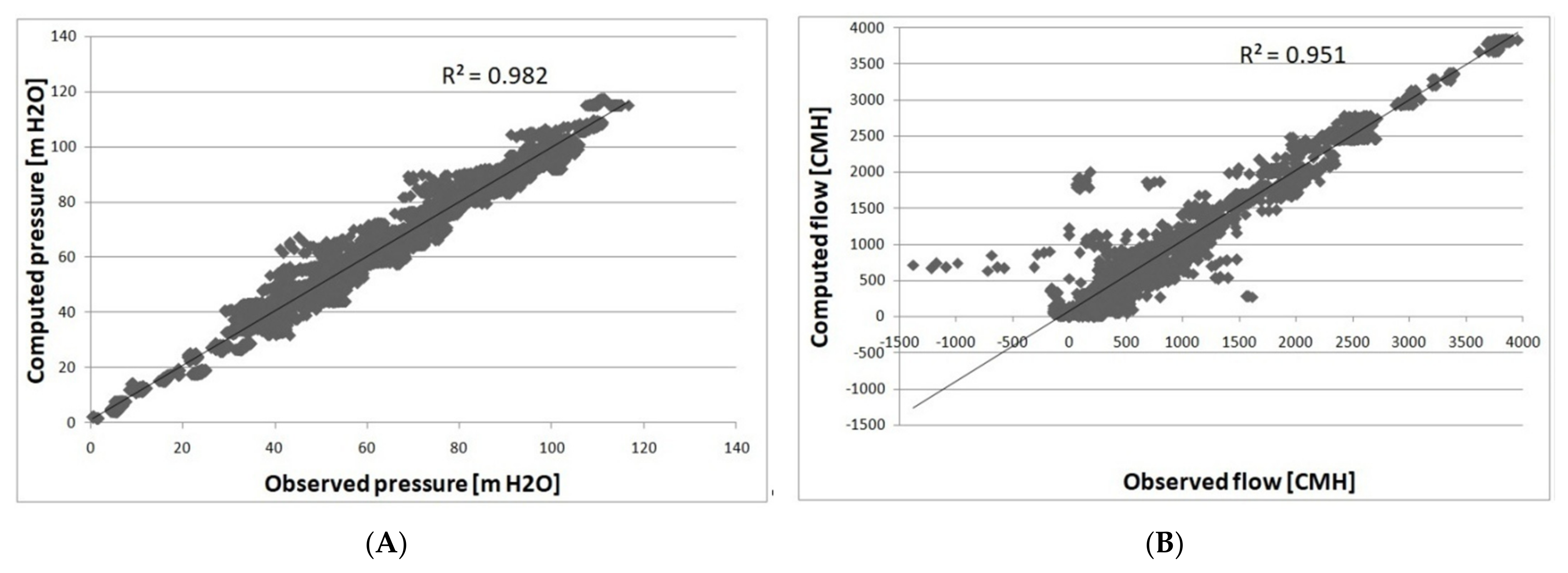
| Number of Measurements | Average Measurement Value | Average Simulation Value | Average Error (%) | Theil | |
|---|---|---|---|---|---|
| Flow (m3/h) | 56 | 974.21 | 1024.69 | 14.11 | 0.01367 |
| Pressure (mH2O) | 118 | 64.23 | 64.65 | 3.70 | 0.00194 |
| PS | Average Pump Efficiency | Pump Power for a Peak Efficiency Point | Operation Time | Energy Consumption |
|---|---|---|---|---|
| (%) | (kW) | (h/week) | (kWh) | |
| WTP B | 75.0 | 501 | 168 | 54,919 |
| WTP B | 75.0 | 413 | 168 | 55,138 |
| WTP C | 100.0 | 412 | 168 | 66,024 |
| WTP D | 63.3 | 290 | 168 | 40,555 |
| WTP E | 73.5 | 86 | 168 | 13,994 |
| WTP F | 33.2 | 171 | 113 | 14,272 |
| WTP G | 52.3 | 311 | 168 | 46,855 |
| WTP H | 49.3 | 520 | 168 | 67,519 |
| WTP I | 71.7 | 119 | 168 | 15,318 |
| WTP I | 61.4 | 108 | 119 | 11,912 |
| WTP I | 57.3 | 35 | 168 | 5712 |
| WTP J | 70.2 | 154 | 168 | 19,824 |
| PS K | 84.5 | 841 | 168 | 139,675 |
| PS L | 80.2 | 701 | 168 | 116,995 |
| PS L | 81.8 | 1375 | 168 | 230,832 |
| PS M | 40.8 | 44 | 149 | 4276 |
| PS M | 67.0 | 76 | 98 | 7330 |
| PS N | 68.6 | 46 | 168 | 6132 |
| PS N | 68.4 | 42 | 152 | 5548 |
| PS N | 70.8 | 54 | 168 | 8350 |
| ST O | 89.2 | 385 | 168 | 61,522 |
| ST S | 67.1 | 37 | 168 | 5342 |
| SUM 998,044 | ||||
| PS | Average Pump Efficiency | Pump Power for a Peak Efficiency Point | Operation Time | Energy Consumption | Reduction of Energy Consumption |
|---|---|---|---|---|---|
| (%) | (kW) | (h/week) | (kWh) | (%) | |
| WTP B | 75.0 | 501 | 168 | 54,934 | 0 |
| WTP B | 75.0 | 426 | 168 | 55,151 | 0 |
| WTP C | 100.0 | 413 | 168 | 60,697 | 8 |
| WTP D | 62.6 | 277 | 168 | 42,437 | −5 |
| WTP E | 73.5 | 86 | 168 | 13,991 | 0 |
| WTP F | 39.5 | 169 | 112 | 14,204 | 0 |
| WTP G | 55.7 | 304 | 168 | 48,871 | −4 |
| WTP H | 44.0 | 381 | 168 | 62,580 | 7 |
| WTP I | 70.1 | 74 | 168 | 9314 | 39 |
| WTP I | Pump off | 100 | |||
| WTP I | 57.3 | 35 | 168 | 5712 | 0 |
| WTP J | 70.3 | 154 | 168 | 19,871 | 0 |
| PS K | 84.6 | 845 | 168 | 140,599 | −1 |
| PS L | 79.2 | 525 | 168 | 86,755 | 26 |
| PS L | 81.8 | 1387 | 168 | 230,530 | 0 |
| PS M | 40.9 | 49 | 149 | 4281 | 0 |
| PS M | 67.0 | 77 | 98 | 7340 | 0 |
| PS N | 68.9 | 42 | 168 | 5700 | 7 |
| PS N | 68.9 | 36 | 152 | 5126 | 8 |
| PS N | 72.5 | 53 | 168 | 8261 | 1 |
| ST O | 89.2 | 385 | 168 | 61,520 | 0 |
| ST S | 68.8 | 37 | 168 | 5201 | 3 |
| SUM | 943,075 | ||||
| PS | Average Pump Efficiency | Pump Power for a Peak Efficiency Point | Operation Time | Energy Consumption | Reduction of Energy Consumption |
|---|---|---|---|---|---|
| (%) | (kW) | (h/week) | (kWh) | (%) | |
| WTP B | 75.0 | 501 | 168 | 57,313 | −4 |
| WTP B | 75.0 | 420 | 168 | 57,514 | −4 |
| WTP C | 100.0 | 413 | 168 | 49,090 | 26 |
| WTP D | 65.8 | 277 | 168 | 39,766 | 2 |
| WTP E | 73.7 | 89 | 168 | 14,599 | −4 |
| WTP F | 42.7 | 169 | 112 | 14,146 | 1 |
| WTP G | 55.8 | 301 | 168 | 47,107 | −1 |
| WTP H | 49.5 | 431 | 168 | 67,620 | 0 |
| WTP I | 70.6 | 74 | 168 | 9190 | 40 |
| WTP I | Pump off | 100 | |||
| WTP I | 57.3 | 35 | 168 | 5715 | 0 |
| WTP J | 70.3 | 154 | 168 | 19,869 | 0 |
| PS K | 84.7 | 845 | 168 | 140,314 | 0 |
| PS L | 78.9 | 525 | 168 | 86,777 | 26 |
| PS L | 80.9 | 1347 | 168 | 222,886 | 3 |
| PSM | Pump off | 100 | |||
| PS M | 66.9 | 73 | 98 | 6896 | 6 |
| PS N | 68.9 | 42 | 168 | 5700 | 7 |
| PS N | 68.9 | 36 | 152 | 5128 | 8 |
| PS N | 72.7 | 53 | 168 | 8261 | 1 |
| ST O | 89.3 | 386 | 168 | 61,651 | 0 |
| ST S | 68.8 | 37 | 168 | 5342 | 0 |
| SUM | 924,885 | ||||
| Energy Consumption | Reduction of Energy Consumption | Environmental Effect Reduction in CO2 Emissions * | ||
|---|---|---|---|---|
| (kWh) | (kWh) | (%) | (kg CO2) | |
| Scenario 1 | 998,044 | - | - | |
| Scenario 2 | 943,075 | 54,969 | 5.5 | 45,696 |
| Scenario 3 | 924,885 | 73,159 | 7.2 | 60,817 |
Publisher’s Note: MDPI stays neutral with regard to jurisdictional claims in published maps and institutional affiliations. |
© 2021 by the authors. Licensee MDPI, Basel, Switzerland. This article is an open access article distributed under the terms and conditions of the Creative Commons Attribution (CC BY) license (https://creativecommons.org/licenses/by/4.0/).
Share and Cite
Zimoch, I.; Bartkiewicz, E.; Machnik-Slomka, J.; Klosok-Bazan, I.; Rak, A.; Rusek, S. Sustainable Water Supply Systems Management for Energy Efficiency: A Case Study. Energies 2021, 14, 5101. https://doi.org/10.3390/en14165101
Zimoch I, Bartkiewicz E, Machnik-Slomka J, Klosok-Bazan I, Rak A, Rusek S. Sustainable Water Supply Systems Management for Energy Efficiency: A Case Study. Energies. 2021; 14(16):5101. https://doi.org/10.3390/en14165101
Chicago/Turabian StyleZimoch, Izabela, Ewelina Bartkiewicz, Joanna Machnik-Slomka, Iwona Klosok-Bazan, Adam Rak, and Stanislav Rusek. 2021. "Sustainable Water Supply Systems Management for Energy Efficiency: A Case Study" Energies 14, no. 16: 5101. https://doi.org/10.3390/en14165101
APA StyleZimoch, I., Bartkiewicz, E., Machnik-Slomka, J., Klosok-Bazan, I., Rak, A., & Rusek, S. (2021). Sustainable Water Supply Systems Management for Energy Efficiency: A Case Study. Energies, 14(16), 5101. https://doi.org/10.3390/en14165101